Abstract
Pharmaceutical and Personal Care Products (PPCPs) have become a significant environmental concern due to their widespread use, persistence, and potential toxicity, often referred to as forever chemicals. This study aims to develop and validate robust in silico models for predicting the aquatic toxicity of PPCPs. To do so, we resorted to the ECOTOX database and employed a Python-based tool to prepare and curate the dataset. Multitasking Quantitative Structure–Toxicity Relationship (mt-QSTR) models were then developed employing the Box–Jenkins moving average approach, incorporating both linear and non-linear frameworks based on diverse feature selection algorithms and machine learning techniques. To further improve the external predictivity, a consensus modeling approach was also implemented. The most accurate model achieved an overall predictive accuracy exceeding 85%, providing valuable insights into the structural features influencing PPCP toxicity. Key factors contributing to high aquatic toxicity included high lipophilicity, mass density, molecular mass, and reduced electronegativity. This work offers a foundation for designing safer PPCPs with reduced environmental impact, aligning with sustainable chemical development goals.
1. Introduction
In the past decade, environmental research has increasingly shifted focus from conventional priority pollutants, such as polychlorinated biphenyls and polycyclic aromatic hydrocarbons, to emerging contaminants. Among these, pharmaceuticals and personal care products (PPCPs) have emerged as a critical group of contaminants of concern [,]. PPCPs span a wide range of chemical substances, including pharmaceuticals for human and veterinary use, disinfectants, and personal care products like lotions, cleansers, and sunscreens. These chemicals enhance our daily lives, from disease prevention to household hygiene.
PPCPs are often only minimally transformed or remain unchanged in wastewater treatment plants, immediately then entering into aquatic environments. Additional sources include direct inputs from aquaculture, indirect inputs through manure application in agriculture, and emissions from manufacturing sites, hospitals, and nursing homes. PPCPs have been detected globally [,], raising concerns due to their large-scale production and usage, persistence in the environment, and toxicity to non-target organisms. Many PPCPs exhibit bioaccumulation potential across different trophic levels, and their continuous emission renders them pseudo-persistent pollutants. Since the mid-1990s, there has been a steady increase in studies assessing the environmental risks posed by PPCPs in both aquatic and terrestrial ecosystems [].
To address the challenge of assessing environmental risks, in silico modeling has been proposed as an efficient alternative to time-consuming and costly experimental methods, particularly under frameworks like the Registration, Evaluation, Authorization, and Restriction of Chemicals (REACH) []. Recent investigations have demonstrated the utility of these in silico techniques in predicting the environmental toxicity of a diverse range of chemical compounds [,,,,,,,,].
Given the significance of PPCPs and the risks they pose to aquatic ecosystems, this work focuses on developing predictive and validated Multitasking Quantitative Structure–Toxicity Relationship (mt-QSTR) models. These models aim to predict the aquatic toxicity of PPCPs using a complex and curated dataset obtained from the ECOTOX database []. The dataset was refined through a newly developed in-house curation tool to ensure accuracy and consistency. To address experimental variations, a Box–Jenkins-based moving average approach was employed, integrating both structural attributes and experimental conditions into the in silico modeling process []. Additionally, a range of feature selection algorithms and machine learning (ML) techniques were applied to identify the most effective linear and non-linear mt-QSTR models, delivering robust predictions of PPCP toxicity.
This work provides valuable insights and a robust framework for designing PPCPs with reduced environmental toxicity, offering a significant step forward in mitigating their impact on aquatic ecosystems.
2. Materials and Methods
Dataset collection and curation. The dataset was collected from ECOTOX database (https://cfpub.epa.gov/ecotox/index.cfm, accessed on 6 June 2024) [] with the following search parameters: (a) habitat: aquatic, (b) chemicals: Pharmaceuticals Personal Care Products (PPCPs), (c) Endpoints: LC (lethal concentration)/LD (lethal dose) xx (all % values) and EC (effective concentration)/ED (effective dose) xx (all % values). This dataset with 2520 entries was properly curated by setting a cut-off value of 5 mg/L, where the Conc 1 Units (Standardized) as Active Ingredient (AI) mg/L were designated as ‘toxic’ ( = +1), whereas the remaining values were selected as ‘non-toxic’ ( = 0). Therefore,
= +1, when Conc 1 Mean (Standardized) value ≤ 5 mg/L
= 0, when Conc 1 Mean (Standardized) value > 5 mg/L
Additionally, two endpoints—EC50 and LC50—were considered for setting up the dataset for modeling. The decision regarding the selection of this cut-off value was guided by the guidelines of Globally Harmonized System of Classification and Labelling of Chemicals (GHS) of the United Nations for estimating toxic doses (https://unece.org/sites/default/files/2021-09/GHS_Rev9E_0.pdf, page 233, accessed on 2 June 2024). Here, if the LC50 (96 h)/EC50 (48 h) value of a chemical is found to be less than 1 mg/L, it comes under the ‘Warning’ or ‘Acute 1’ category for aquatic toxicity. In contrast, those chemicals with LC50 (96 h)/EC50 (48 h) values between 1 and 10 mg/L belong to the ‘Acute 2’ category. Therefore, a cut-off value of 5 mg/L may be selected so that most of the ‘Acute 1’ chemicals are assigned as “toxic” irrespectively of the experimental protocol.
Generally, for any given cut-off value and experimental conditions, the ECOTOX dataset may contain several duplicated data points. Since mt-QSTR modeling was performed using the Box–Jenkins approach, it was essential to determine which experimental conditions should be included as factors for classification modeling. In this work, we used five experimental conditions, viz. (a) species scientific name (sn), (b) species group (sg), (c) concentration 1 type (standardized) (co), (d) endpoint (ep), and (e) time of exposure (te). Save for te, all other experimental elements were directly obtained from the downloaded ECOTOX dataset. The te element was derived from the exposure time [column name: ‘Observed Duration Units (Days)’ from ECOTOX dataset], where datapoints with values between 0 and 4 days were designated as ‘Short’, values between 4 and 10 days were set as ‘Medium’, and values with greater than 10 days were denoted as ‘Long’.
The next challenge was identifying and processing duplicated data points. In conventional single-target QSTR, data points are considered duplicated when identical chemical structures appear multiple times with varying experimental results. Such duplicates can be easily identified by examining the canonical SMILES of the compounds in the dataset. However, in the case of mt-QSTR, the concept of a “data point” is more complex. Here, each data point represents a combination of a chemical structure and its associated experimental conditions included for modeling. Therefore, two data points can be considered duplicated only when both the canonical SMILES and the experimental conditions are identical. This complexity makes dataset curation for multi-target QSTR significantly more challenging, requiring extensive manual effort. To address this, we utilized an in-house open-access tool called Ecotox-curator (available at https://github.com/ncordeirfcup/Ecotox-curator, accessed on 14 June 2024), which provides a graphical user interface (GUI) for automated data curation, starting from datasets downloaded from the ECOTOX database. The overall methodology of this tool for data curation is delineated in Figure 1.
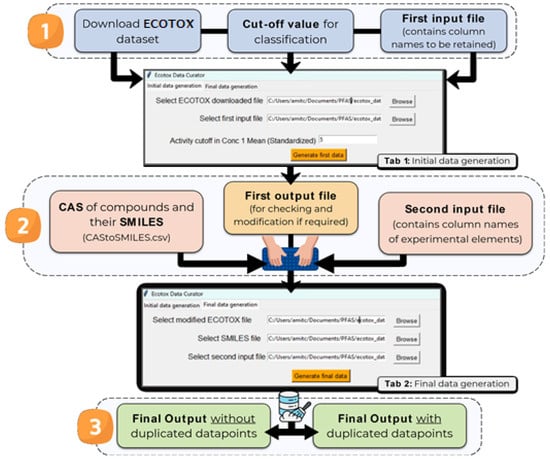
Figure 1.
Methodology adopted for data curation for mt-QSTR modeling using the Ecotox-curator tool.
Briefly, Ecotox-curator assists users in a two-step data curation process:
- Data Selection and Preprocessing: Users provide the downloaded raw ECOTOX dataset file (.csv format), and a separate file (“First_input.csv”) specifying the desired columns for further processing. For example, in this work, the input file contains columns and values such as (a) SN—a serial number manually created to track the data points in the original dataset, (b) CAS number (required), (c) Chemical name, (d) Species Scientific Name, (e) Species Group, (f) Conc 1 Type (Standardized), (g) Conc 1 Mean Op (Standardized), (h) Conc 1 Mean (Standardized), (i) Conc 1 Units (Standardized): AI mg/L, (j) Endpoint: LC50, EC50, and (k) Observed Duration (Days).
- Additionally, the tool requires a specific cut-off value to define ‘toxic’ and ‘non-toxic’ classes. As mentioned earlier, a cut-off value of 5 mg/L was used in this work. The tool automatically saves a new file (“FirstFile_forChecking.csv”) containing the specified columns along with the activity column (i.e., ‘Active’). Basically, in this stage, the tool collects those columns that are necessary for modeling and removes unnecessary data, as specified by the users. Users can then manually check and modify “FirstFile_forChecking.csv” if necessary. For example, we created a new ‘Time’ category (Long, Medium, Short) based on the ‘Observed Duration (Days)’ column and removed irrelevant values like “NR” (Not Reported).
- Duplicate Removal and Conflict Resolution: Once satisfied with the preliminary data, users should upload the modified “FirstFile_forChecking.csv” and a separate file (“CAStoSMILES.csv”) linking CAS numbers to their corresponding SMILES notations (which ECOTOX does not provide). Tools like the Python-based CIRpy (available at https://github.com/mcs07/CIRpy, accessed on 16 June 2024) can assist in SMILES generation, but manual correction might be needed for CAS number formatting (missing hyphens in ECOTOX data). Alongside these two files, another input file (“Second_input.csv”) is needed at this stage. This file specifies the column names to be treated as final experimental elements for further processing. In this work, the following column names were included: (a) Species Scientific Name (sn); (b) Species Group (sp); (c) Conc 1 Type (Standardized); (d) Endpoint; and (e) Time. In this stage, the duplicated data points are identified from the SMILES notations and experimental elements. Finally, the tool generates two output files:
- “NoDuplicates.csv”: Contains data points without duplicates or duplicates with consistent activity classifications (all toxic or all non-toxic). Data points from this file are used for model development and validation.
- “DupConflict.csv”: Contains data points with conflicting duplications (e.g., data points classified as both ‘toxic’ and ‘non-toxic’). Data points from this file were not considered for modeling since conflicting activity classes were found.
Descriptor calculation. In this study, 1141 EPA (T.E.S.T.) descriptors (797 2D descriptors and 344 3D descriptors) were calculated for the dataset compounds using the OCHEM webserver []. These descriptors were generated through the Toxicity Estimation Software Tools (T.E.S.T.) available on the United States Environmental Protection Agency (EPA) website (https://www.epa.gov/comptox-tools/toxicity-estimation-software-tool-test, accessed on 28 June 2024). For the 3D descriptors, geometrical optimization of the chemical structures of the dataset compounds was carried out by employing the quantum chemical semi-empirical PM6 method through ULYSSES [] on the OCHEM platform.
The descriptors were then processed with the in-house open-access software QSAR-Co-X (available at https://github.com/ncordeirfcup/QSAR_Co_X_v2, accessed on 4 July 2024), which was specifically designed for developing Multitasking Quantitative Structure–Toxicity Relationship (mt-QSTR) classification models using the Box–Jenkins moving average (BJMA) technique []. A detailed description of the BJMA technique, including its applications and scope, can be found elsewhere [,,]. Note that the ‘QSAR-Co-X’ term is derived from Quantitative Structure Activity Relationship with COnditions eXtended version.
To begin with, the dataset was split into training (70%) and validation (30%) sets using k-means cluster analysis (k-MCA), with five clusters and a random state of 42. This method ensures a uniform and representative distribution of the dataset by grouping data points based on diversity derived from the response variable and the calculated descriptors [,,]. After the initial split, the BJMA technique was applied to the training set to calculate deviation descriptors using the ‘Method-1’ option in QSAR-Co-X []. This option uses the simplest form of BJMA to calculate the deviation descriptors ∆(Di)cj, as follows:
Specifically, the new descriptors, i.e., the deviation descriptors, are calculated for a unique experimental condition (ontology), cj, by the difference between the input descriptors (Di) and the arithmetic mean from positive samples (‘toxic’, or +1 in our case) associated with a specific element from this ontological condition. This stage yielded a training set with deviation descriptors, while the obtained avg(Di)cj descriptors were also deployed to determine the validation set’s deviation descriptors.
The training dataset was further divided into a sub-training set (80%) and a test set (20%) using a random seed (42). We then developed the models using solely this sub-training dataset and estimated their external predictive performance using both the test and validation sets. Since the validation set is independent of both descriptor calculation and model development, it provides a true measure of the model’s predictive power. In contrast, the test set, while not used for model development, is involved in descriptor calculation. If the test set’s predictive accuracy is significantly higher than the validation set’s, the model may be biased towards the moving average technique. In such cases, the validation set’s prediction becomes more reliable for assessing the model’s true external predictive ability. To conclude this phase, prior to model development, a preprocessing step removed highly correlated (>0.95) and near-constant descriptors (variance < 0.001) to improve model performance.
Linear modeling. In this study, we employed linear discriminant analysis (LDA) coupled with three feature selection algorithms: fast-stepwise selection (FS), stepwise forward selection (SFS), and genetic algorithm (GA). Each LDA model was limited to a maximum of ten descriptors.
FS-LDA models relied on p-values for feature selection. SFS-LDA models were generated using the Python-based Mlxtend library (http://rasbt.github.io/mlxtend/, accessed on 4 July 2024) by varying scoring functions like accuracy and AUROC (area under the receiver operating characteristic curve) obtained from QSAR-Co-X []. For each SFS scoring function, different models were set up using various cross-validation (CV) techniques, i.e., no CV, 5-fold CV, and 10-fold CV. In contrast, GA, implemented with the in-house Java-based open-access tool QSAR-Co (https://sites.google.com/view/qsar-co, accessed on 10 July 2024) [], is a stochastic method. This means each run generates new models due to variations in the randomized data. Therefore, we ran GA-LDA at least 100 times (reopening the software after every 20 runs) to ensure sufficient exploration.
Non-linear modeling. Recent advancements in non-linear modeling have markedly improved the analysis and interpretation of big data, offering powerful tools to extract meaningful insights. To harness this potential, we utilized a comprehensive suite of machine learning techniques coupled with the following feature selection algorithms to identify the most predictive non-linear models:
- Linear model descriptors, where only descriptors from the most predictive linear model are selected.
- All descriptors, where all pre-treated descriptors are subjected to modeling.
- Random forest importance, where the random forest (RF) classifier is employed to select the most significant descriptors, with the help of Scikit-learn library [].
- Recursive feature elimination (RFE), where the decision tree classifier is used as an estimator for descriptor selection. In RFE, a user-defined classifier is trained on the initial set of features, then feature importance is recorded and the least important ones are eliminated; this procedure is repeated recursively on the pruned set until a user-defined number of features are left.
- Sequential forward selection (SFS), where SFS is applied for feature selection sequentially with a defined scoring function (e.g., accuracy), whereas a specific user-defined ML tool is applied for model evaluation. In this case, the Mlxtend library is used for SFS feature selection, and the decision tree classifier (DTC) of Scikit-learn is employed for model evaluation.
- Genetic algorithm and k-nearest neighborhood (GA-kNN), where the Python-based sklearn-genetic module (https://github.com/manuel-calzolari/sklearn-genetic, accessed on 12 July 2024) is utilized to explore a ‘deap’ function for running GA, with the following parameters: population (100), mutation probability (0.2), cross-over probability (0.5), number of generations (100), number of generations no change (10), crossover independent probability (0.1), mutation independent probability (0.05), and fixed kNN parameters (‘12’ number of neighbors, ‘uniform’ weights, and ‘auto’ algorithm), whereas 5-fold CV is used along with accuracy scores for model evaluation. Note that in this tool, the stochastic GA method is used for descriptor selection, but each model is evaluated with kNN [].
For each feature selection algorithm, we applied five machine learning techniques: k-Nearest Neighbors []; random forest (RF) []; Support Vector Classifier (SVC) []; Multilayer Perceptron (MLP) [], and Gradient Boosting (GB) []. QSAR-Co-X_v2 software’s ‘Module-2’ was used to generate these ML models on the sub-training set. Hyperparameter optimization was performed during model development, with parameters explored as described in the original QSAR-Co-X article []. The parameters optimized for the various ML techniques are described in Table S2. A 5-fold cross-validation was employed for both hyperparameter optimization and model evaluation. A random seed value of 42 was used consistently throughout the process. Finally, we evaluated the predictive performance of the optimized models on both the test and validation sets.
Model evaluation and reliability. The predictive performance of the final classification models was assessed using a range of well-established statistical parameters, calculated by the QSAR-Co-X tool. Formulas for these parameters—sensitivity, specificity, accuracy, and Matthew’s correlation coefficient (MCC) [,,]—are given in Table 1. For model selection, we primarily relied on MCC, which is considered a stringent and reliable metric for evaluating the predictive quality of classification models, especially when dealing with imbalanced datasets. Additionally, receiver operating characteristic (ROC) curves were generated to provide a graphical representation of model performance. Essentially, the ROC curve plots the true positive rate (TPR) against the false positive rate (FPR) across various classification thresholds. The area under the ROC curve (AUROC) was also calculated, offering a quantitative measure of the model’s ability to distinguish between classes.

Table 1.
Formulas for key statistical parameters used in the present work to evaluate the quality of classification-based mt-QSTR models.
Furthermore, we employed two complementary techniques for determining the applicability domain (AD) of our mt-QSTR models. First, the standardization-based AD method, proposed by Roy et al. [], was utilized. This method identifies outliers and confirms if predictions remain within the defined model domain. All calculations related with this method were performed with the QSAR-Co-X software. Second, we applied the confidence estimation approach, also developed by Roy et al. [], with a threshold value of 0.25. This technique assesses the reliability of predictions based on their proximity to the training data. Both methodologies have been comprehensively explained in a previous study [], providing robust measures to evaluate the reliability and applicability of the developed mt-QSTR models.
Consensus modeling. Recent years have seen the introduction of the concept of consensus modeling, which posits that combining the most predictive models will invariably enhance model performance, ensuring the final model’s maximum predictive capability []. In this work, we employed the newly introduced ‘Module5.py’ module within QSAR-Co-X software to automatically perform consensus modeling on our models. It is important to note that when using an odd number of models, the software employs a majority voting system to handle predictions with uneven distributions. However, for an even number of models, this method is only applicable when there are at least four models, and the predictive distributions are not uniform. For an even number of models with 50% predictions as ‘toxic’ (or +1) and 50% as ‘non-toxic’ (or 0), such rule is not applicable, and predictions are based on posterior probabilities. The prediction with maximum posterior probability is then considered as the final prediction.
3. Results and Discussions
Data curation results. Firstly, it was essential to analyze the two output files—NoDuplicates.csv and DupConflict.csv—obtained from the data curation process using the Ecotox-curator tool. From the original dataset, 1150 non-duplicated and unique data points were retrieved, pertaining to different experimental conditions, chemical structures, and response variables. These curated data points (Table S1) were utilized for model development and validation. Specifically, 88 unique chemical structures of PPCPs were found, along with the five different experimental elements considered (i.e., sn, sg, te, co, and ep). By ascertaining a toxicity cut-off of 5 mg/L, the dataset for mt-QSTR modeling comprised 603 toxic and 547 non-toxic data points. As such, the dataset is well-balanced for classification modeling.
Development and validation of mt-QSTR models. Following the strategy previously outlined, we began by employing the k-MCA technique to divide our dataset into sub-training (Nstr = 641), test (Nts = 161), and validation (Nvd =348) sets. We then first developed linear discriminant analysis models by applying the three types of feature selection techniques, i.e., FS, SFS, and GA. Multiple SFS-LDA models were built by adjusting scoring functions and cross-validation methods. The statistical results of the eight obtained LDA models are summarized in Table 2, based on their MCC values for the sub-training and test sets.
Table 2.
Summary of statistical quality of the linear mt-QSAR models (L01-L08) developed using LDA coupled with different feature selection (FS) techniques.
As seen, the GA-LDA method-generated Model L08 provides the maximum average MCC values for the sub-training and test sets. This model was subsequently used to determine its external predictivity against the validation set, where it achieved an MCC value of 0.589. The detailed statistical results of Model L08 are presented in Table 3.
Table 3.
Detailed statistical results of the linear mt-QSTR model L08.
From Table 3, it is evident that the model achieves an overall accuracy of approximately 86%, correctly predicting 989 data points. However, the external predictivity towards the validation set remains only moderate. Therefore, to ensure that L08 represents the optimal mt-QSTR model, it was crucial to investigate alternative model development strategies. This involved exploring non-linear modeling approaches, employing the five machine learning techniques (kNN, RF, SVC, MLP, and GB) along with the six feature selection algorithms (descriptors from L08 model, all descriptors, RFE, RF-importance, SFS, and GA-kNN) as detailed in the previous section.
In so doing, 30 non-linear models were developed, and rigorous hyperparameter optimization was performed for each to identify the most suitable model parameters. The performance metrics for these models are summarized in Table 4. While six non-linear models demonstrated superior predictive performance compared to the best linear model (L08) on the sub-training and test sets, this advantage did not translate to improved performance on the independent validation set. This observation suggests a potential for overfitting within the non-linear models, hindering their ability to generalize beyond the training data and thus limiting their ability to surpass the predictive accuracy of the linear model.
Table 4.
Summary of the results obtained for the 30 non-linear developed mt-QSTR models.
As a final resort, we relied on the consensus model generation technique to check if combining predictions from multiple models would improve predictivity towards the validation set. For consensus prediction, we selected the most predictive linear model, L08, and four non-linear models: NL06, NL10, NL16, and NL30 (cf. Table 4), which demonstrated satisfactory predictivity (MCC > 0.5) towards the validation set. Although four consensus models achieved MCC > 0.55 for the validation set (see Table S3), none surpassed the performance of L08 in terms of external predictivity towards the validation set. Therefore, the linear model L08 stood out as the most predictive mt-QSTR model generated for tackling the environmental toxicity of PPCPs.
Further support for the model’s suitability is provided by the ROC plot (see Figure 2), clearly indicating that the L08 model is not random but a statistically significant classifier. Additionally, inspecting the correlation matrix of its deviation descriptors confirmed that high inter-collinearity (R > 0.95) did not exist among them.
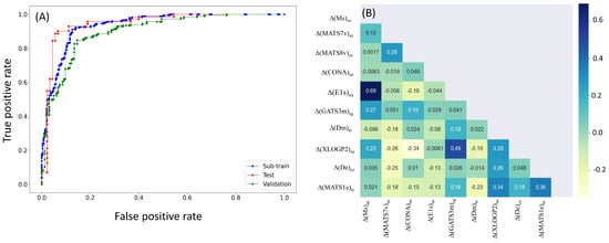
Figure 2.
ROC plot of the L08 model (A) and inter-correlation among its deviation descriptors (B).
Moreover, establishing the applicability domain of the model is also deemed necessary. When applying the standardization approach, 31, 11, and 25 data points were detected as structural outliers for the sub-training, test, and validation sets, respectively, and their removal led to MCC values of 0.772, 0.826, and 0.593, respectively. The confidence estimation approach, which may be more important for outlier determination in mt-QSTR modeling, especially for the validation set, estimates the level of confidence with which a model may predict a data point. Using a threshold value of 0.25, 48 outliers were detected in the sub-training set, and their removal increased the MCC score to 0.802. The test and validation sets had 17 and 36 outliers, respectively, and removing these outliers resulted in new MCC values of 0.83 and 0.63, respectively.
The significance of the descriptors of the L08 model was estimated by their standardized coefficients, the results of which are depicted in Figure 3. The meaning of these deviation descriptors is outlined in Table 5.
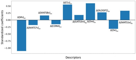
Figure 3.
Contribution of deviation descriptors in the linear L08 model.
Table 5.
Description of the deviation descriptors in the linear L08 model.
Noticeably, save for the endpoint (ep), all experimental elements selected in the present work were found in the mt-QSTR model, indicating the importance of each. However, the ‘Species scientific name’ (sn) appeared the most frequently (five times), while both the ‘Time of experiment’ (te) and ‘Concentration type’ (co) were found in two deviation descriptors each. Meanwhile, the ‘Species group’ (sg) was found in only one deviation descriptor.
The ∆(Ms)sn descriptor, relating to the experimental element sn, indicates that a higher value of this descriptor is responsible for lower aquatic toxicity. Generally, the presence of polar atoms (such as N, O, F, Cl, etc.) and unsaturation increases the value of Ms in compounds. In Figure 4, some correctly predicted PPCPs with low and high values of ∆(Ms)sn are presented. Naturally, compounds with fewer polar residues (compared to the total number of atoms) were found to have lower values of this descriptor.
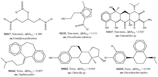
Figure 4.
Examples of data points to explain the contribution of ∆(Ms)sn to aquatic toxicity.
Evidently, compounds with low Ms values may have a higher chance of increased lipophilicity due to the lack of electronegative atoms. This is further corroborated by the fact that the lipophilicity-based descriptor ∆(XLOGP2)sn was found to be positively correlated with the response variable of the model []. As depicted in Figure 5, some data points with high values of ∆(XLOGP2)sn were indeed found to be toxic, whereas low values for this deviation descriptor were observed in non-toxic PPCPs.
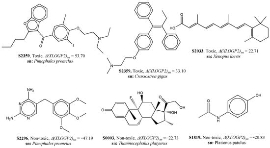
Figure 5.
Examples of data points to explain the contribution of ∆(XLOGP2)sn to aquatic toxicity.
However, the mt-QSTR model itself suggests a more complex relationship between structural attributes and toxicity. Even though Ms is simply a constitutional descriptor, the second most significant descriptor of the model, ∆(Dm)te, is based on the 3D Weighted Holistic Invariant Molecular (WHIM) descriptor D total accessibility index (weighted by mass) []. WHIM descriptors represent the entire 3D-molecular structure in terms of size, shape, symmetry, and atom distribution. Previously, WHIM descriptors were recommended for environmental modeling []. Generally, the values of 3D WHIM descriptors depend strongly on the 3D conformations of chemical structures [].
In this work, we relied on the semi-empirical quantum chemical technique for geometrical optimization of the dataset compounds. To check how the 3D conformations influence the quality of the generated model, we generated models with descriptors calculated from dataset compounds optimized using the molecular mechanics force field under OCHEM webserver’s ‘Rdkit’ option. The new model showed significantly low predictivity for both sub-training and test sets (i.e., MCC values of 0.723 and 0.762, respectively).
Additionally, the Dm descriptor is heavily dependent on the molecular density (molecular mass/molecular volume) of compounds. Significantly, the presence of heavy atoms (e.g., Cl, I) responsible for higher molecular density may increase the risk of environmental toxicity. This is exemplified in Figure 6, which shows correctly predicted toxic compounds with high values of ∆(Dm)te and non-toxic compounds with low values of this descriptor. Conversely, non-toxic compounds lack such atoms. Simultaneously, another descriptor, ∆(De)co, also based on a D-type WHIM descriptor, was negatively correlated to toxicity. The De descriptor is weighted by electronegativity, and thus, compounds with an increased number of polar atoms are less likely to induce aquatic toxicity.
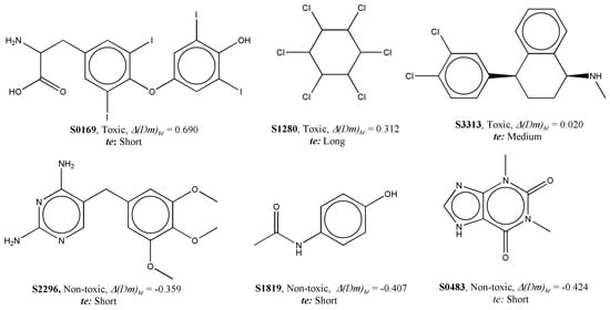
Figure 6.
Examples of data points to explain the contribution of ∆(Dm)te to aquatic toxicity.
Interestingly, even though ∆(Ms)sn was found to have the maximum influence on the model, it is not the only intrinsic state-weighted descriptor. The ∆(E1s)sn is another WHIM descriptor that is weighted by the intrinsic state. Noticeably, even though ∆(Ms)sn and ∆(E1s)sn are both based on the experimental element sn and weighted by the intrinsic state (s), they have opposite relationships with the response variable. Therefore, a balance between these descriptors is responsible for determining the toxicity of the PPCPs.
More importantly, the 2D and 3D topology of the compounds largely influences their toxicity. It is observed that two closely related descriptors, ∆(MATS7v)sn and ∆(MATS8v)sn, have opposite relationships with the dependent parameter. Both MATS7v and MATS8v are Moran 2D autocorrelation descriptors weighted by van der Waals volume []. The difference lies in their topological path lengths, which are 7 and 8 for these two descriptors, respectively. As shown in the correlation matrix (cf. Figure 2), these two descriptors (i.e., ∆(MATS7v)sn and ∆(MATS8v)sn) do not show high inter-collinearity. However, the difference in their contributions to the model indicates that a slight change in the chemical structure may significantly alter its environmental toxicity.
On the other hand, another Moran autocorrelation descriptor ∆(MATS1e)te also contributed positively to the model. Among different atomic properties, atomic mass depicted consistency in contributions for the descriptors weighted by it. For example, both ∆(GATS3m)sg and ∆(Dm)te were found to be positively correlated to toxicity. Therefore, it is inferred that PPCPs with higher molecular weights are more prone to elicit aquatic toxicity when the species groups and time of experiments are varied.
Comparison of present findings to prior investigations. Previous investigations into the toxicity of pharmaceuticals and personal care products have focused on specific compounds or limited experimental conditions [,,,,]. This study aims to develop an mt-QSTR model that encompasses a broader range of experimental conditions and diverse chemical structures from the ECOTOX database. Consequently, the scope of this model surpasses previous reports.
A key advantage of mt-QSTR modeling lies in its applicability to a wide array of chemicals and experimental settings. Recognizing the continuous growth of chemical databases like ECOTOX, this work emphasizes reproducible methodologies. Open-access tools and readily adaptable codes are provided to facilitate the development of future QSTR models not only for PPCPs but also for other types of chemicals with environmental toxicity risks.
4. Conclusions
In this work, the Box–Jenkins-based moving average approach was adopted to set up validated and predictive mt-QSTR models. Linear and non-linear models were developed using a range of feature selection algorithms and machine learning techniques. Notably, it is the LDA technique that produced the most statistically significant model (L08), which outperformed both non-linear and subsequent consensus models.
The linear model clearly demonstrated the contributions of various deviation descriptors. The PPCPs in the current dataset cover a large chemo-biological space, and their complexity is reflected in the L08 model, where complex graph-based topological descriptors predominate over simple, interpretable descriptors. It is well known that factors such as lipophilicity and water solubility of the compounds play crucial roles in the aquatic toxicity of chemicals. Indeed, our linear model suggests that intrinsic factors, such as mass and van der Waals volume of the atoms, play pivotal roles.
Closely related descriptors (e.g., ∆(MATS7v)sn and ∆(MATS8v)sn) were found to have opposite relationships with the response variable. Nevertheless, the descriptor with the maximum contribution was ∆(Ms)sn. The model indicates the contribution of lipophilicity in the form of the descriptor ∆(XLOGP2)sn and explains that the presence of heavy atoms, such as Cl and I, increases the risk of environmental toxicity. Similarly, low molecular weight PPCPs with an increased number of electronegative elements (N, O, etc.) have less potential to elicit aquatic toxicity.
Clearly, the developed model can be used to predict the aquatic toxicity of new PPCPs and help design new PPCPs with low environmental toxicity. This work not only focuses on model generation but also paves the way for dataset curation in an automated fashion with the help of our in-house software, Ecotox-curator, which may be employed in the future for performing mt-QSTR modeling.
Supplementary Materials
The following supporting information can be downloaded at: https://www.mdpi.com/article/10.3390/app15031246/s1; Table S1: List of the curated data points utilized for model development and validation; Table S2: Hyperparameters optimized for generating machine learning models. Table S3: Possible consensus models, resulting from a combination of the several developed models.
Author Contributions
Conceptualization, A.K.H. and M.N.D.S.C.; formal analysis, A.K.H. and T.P.; data curation, A.K.H. and T.P.; funding acquisition, M.N.D.S.C.; investigation, A.K.H., T.P. and M.N.D.S.C.; methodology, A.K.H. and M.N.D.S.C.; software, A.K.H. and M.N.D.S.C.; project administration, M.N.D.S.C.; supervision, A.K.H. and M.N.D.S.C.; validation, A.K.H., T.P. and M.N.D.S.C.; writing—original draft, A.K.H. and T.P.; writing—review and editing, A.K.H. and M.N.D.S.C. All authors have read and agreed to the published version of the manuscript.
Funding
This work received financial support from the PT national funds (FCT/MCTES, Fundação para a Ciência e Tecnologia and Ministério da Ciência, Tecnologia e Ensino Superior) through the project UID/50006—Laboratório Associado para a Química Verde—Tecnologias e Processos Limpos.
Institutional Review Board Statement
Not applicable.
Informed Consent Statement
Not applicable.
Data Availability Statement
The original contributions presented in this study are included in the article/Supplementary Materials. Further inquiries can be directed to the corresponding author.
Conflicts of Interest
The authors declare no conflicts of interest.
References
- Bu, Q.; Wang, B.; Huang, J.; Deng, S.; Yu, G. Pharmaceuticals and personal care products in the aquatic environment in China: A review. J. Hazard. Mater. 2013, 262, 189–211. [Google Scholar] [CrossRef] [PubMed]
- Wang, H.; Xi, H.; Xu, L.; Jin, M.; Zhao, W.; Liu, H. Ecotoxicological effects, environmental fate and risks of pharmaceutical and personal care products in the water environment: A review. Sci. Total Environ. 2021, 788, 147819. [Google Scholar] [CrossRef] [PubMed]
- Chakraborty, A.; Adhikary, S.; Bhattacharya, S.; Dutta, S.; Chatterjee, S.; Banerjee, D.; Ganguly, A.; Rajak, P. Pharmaceuticals and personal care products as emerging environmental contaminants: Prevalence, toxicity, and remedial approaches. ACS Chem. Health Saf. 2023, 30, 362–388. [Google Scholar] [CrossRef]
- Srain, H.S.; Beazley, K.F.; Walker, T.R. Pharmaceuticals and personal care products and their sublethal and lethal effects in aquatic organisms. Environ. Rev. 2021, 29, 142–181. [Google Scholar] [CrossRef]
- Chinen, K.; Malloy, T. Multi-strategy assessment of different uses of QSAR under REACH analysis of alternatives to advance information transparency. Int. J. Environ. Res. Public Health 2022, 19, 4338. [Google Scholar] [CrossRef]
- Belfield, S.J.; Firman, J.W.; Enoch, S.J.; Madden, J.C.; Tollefsen, K.E.; Cronin, M.T.D. A review of quantitative structure-activity relationship modelling approaches to predict the toxicity of mixtures. Comput. Toxicol. 2023, 25, 100251. [Google Scholar] [CrossRef]
- Halder, A.K.; Moura, A.S.; Cordeiro, M.N.D.S. Predicting the ecotoxicity of endocrine disruptive chemicals: Multitasking in silico approaches towards global models. Sci. Total Environ. 2023, 889, 164337. [Google Scholar] [CrossRef] [PubMed]
- Heo, S.; Safder, U.; Yoo, C. Deep learning driven QSAR model for environmental toxicology: Effects of endocrine disrupting chemicals on human health. Environ. Pollut. 2019, 253, 29–38. [Google Scholar] [CrossRef] [PubMed]
- Sheffield, T.Y.; Judson, R.S. Ensemble QSAR modeling to predict multispecies fish toxicity lethal concentrations and points of departure. Environ. Sci. Technol. 2019, 53, 12793–12802. [Google Scholar] [CrossRef]
- Na, M.; Nam, S.H.; Moon, K.; Kim, J. Development of a nano-QSAR model for predicting the toxicity of nano-metal oxide mixtures to Aliivibrio fischeri. Environ. Sci. Nano 2023, 10, 325–337. [Google Scholar] [CrossRef]
- Halder, A.K.; Cordeiro, M.N.D.S. Probing the environmental toxicity of deep eutectic solvents and their components: An in silico modeling approach. ACS Sustain. Chem. Eng. 2019, 7, 10649–10660. [Google Scholar] [CrossRef]
- Rybinska, A.; Sosnowska, A.; Grzonkowska, M.; Barycki, M.; Puzyn, T. Filling environmental data gaps with QSPR for ionic liquids: Modeling n-octanol/water coefficient. J. Hazard. Mater. 2016, 303, 137–144. [Google Scholar] [CrossRef] [PubMed]
- Khan, P.M.; Sanderson, H.; Roy, K. QSTR and interspecies-QSTR modelling for aquatic toxicity data gap filling of cationic polymers. Comput. Toxicol. 2021, 20, 100181. [Google Scholar] [CrossRef]
- Du, R.; Zhang, Q.; Wang, B.; Huang, J.; Deng, S.; Yu, G. Quantitative structure-activity relationship models for the reaction rate coefficients between dissolved organic matter and PPCPs. J. Hazard. Mater. 2023, 458, 131845. [Google Scholar] [CrossRef] [PubMed]
- Olker, J.H.; Elonen, C.M.; Pilli, A.; Anderson, A.; Kinziger, B.; Erickson, S.; LaLone, C.A.; Russom, C.L.; Hoff, D. The ECOTOXicology knowledgebase: A curated database of ecologically relevant toxicity tests to support environmental research and risk assessment. Environ. Toxicol. Chem. 2022, 41, 1520–1539. [Google Scholar] [CrossRef]
- Halder, A.K.; Moura, A.S.; Cordeiro, M.N.D.S. Moving average-based multitasking in silico classification modeling: Where do we stand and what is next? Int. J. Mol. Sci. 2022, 23, 4937. [Google Scholar] [CrossRef]
- Sushko, I.; Novotarskyi, S.; Körner, R.; Pandey, A.K.; Rupp, M.; Teetz, W.; Brandmaier, S.; Abdelaziz, A.; Prokopenko, V.V.; Tanchuk, V.Y.; et al. Online chemical modeling environment (OCHEM): Web platform for data storage, model development and publishing of chemical information. J. Comput.-Aided Mol. Des. 2011, 25, 533–554. [Google Scholar] [CrossRef]
- Menezes, F.; Popowicz, G.M. ULYSSES: An efficient and easy to use semiempirical library for C++. J. Chem. Inf. Model. 2022, 62, 3685–3694. [Google Scholar] [CrossRef] [PubMed]
- Halder, A.K.; Cordeiro, M.N.D.S. QSAR-Co-X: An open source toolkit for multitarget QSAR modelling. J. Cheminform. 2021, 13, 29. [Google Scholar] [CrossRef]
- Ambure, P.; Halder, A.K.; Gonzalez-Diaz, H.; Cordeiro, M.N.D.S. QSAR-Co: An open source software for developing robust multitasking or multitarget classification-based QSAR models. J. Chem. Inf. Model. 2019, 59, 2538–2544. [Google Scholar] [CrossRef]
- Gower, J.C. A comparison of some methods of cluster analysis. Biometrics 1967, 23, 623–637. [Google Scholar] [CrossRef]
- Beauchaine, T.P.; Beauchaine, R.J., 3rd. A comparison of maximum covariance and K-means cluster analysis in classifying cases into known taxon groups. Psychol. Methods 2002, 7, 245–261. [Google Scholar] [CrossRef] [PubMed]
- Zhao, L.; Fang, J.; Ji, Y.; Zhang, Y.; Zhou, X.; Yin, J.; Zhang, M.; Bao, W. K-means cluster analysis of characteristic patterns of allergen in different ages: Real life study. Clin. Transl. Allergy 2023, 13, e12281. [Google Scholar] [CrossRef] [PubMed]
- Pedregosa, F.; Varoquaux, G.; Gramfort, A.; Michel, V.; Thirion, B.; Grisel, O.; Blondel, M.; Prettenhofer, P.; Weiss, R.; Dubourg, V.; et al. Scikit-learn: Machine learning in python. J. Mach. Learn. Res. 2011, 12, 2825–2830. [Google Scholar]
- Cover, T.; Hart, P. Nearest neighbor pattern classification. IEEE Trans. Inf. Theory 1967, 13, 21–27. [Google Scholar] [CrossRef]
- Breiman, L. Random forests. Mach. Learn. 2001, 45, 5–32. [Google Scholar] [CrossRef]
- Guang-Bin, H.; Babri, H.A. Upper bounds on the number of hidden neurons in feedforward networks with arbitrary bounded nonlinear activation functions. IEEE Trans. Neural Netw. 1998, 9, 224–229. [Google Scholar] [CrossRef] [PubMed]
- Friedman, J.H. Greedy function approximation: A gradient boosting machine. Ann. Stat. 2001, 29, 1189–1232. [Google Scholar] [CrossRef]
- Fawcett, T. An introduction to ROC analysis. Pattern Recognit. Lett. 2006, 27, 861–874. [Google Scholar] [CrossRef]
- Zou, Q.; Boughorbel, S.; Jarray, F.; El-Anbari, M. Optimal classifier for imbalanced data using Matthews Correlation Coefficient metric. PLoS ONE 2017, 12, e0177678. [Google Scholar] [CrossRef]
- Roy, K.; Kar, S.; Ambure, P. On a simple approach for determining applicability domain of QSAR models. Chemom. Intell. Lab. Syst. 2015, 145, 22–29. [Google Scholar] [CrossRef]
- Ambure, P.; Bhat, J.; Puzyn, T.; Roy, K. Identifying natural compounds as multi-target-directed ligands against Alzheimer’s disease: An in silico approach. J. Biomol. Struct. Dyn. 2018, 37, 1282–1306. [Google Scholar] [CrossRef] [PubMed]
- Kier, L.B.; Hall, L.H. An Electrotopological-state Index for Atoms in Molecules. Pharm. Res. 1990, 7, 801–807. [Google Scholar] [CrossRef]
- Wang, J.; Wang, W.; Huo, S.; Lee, M.; Kollman, P.A. Solvation Model based on weighted solvent accessible surface area. J. Phys. Chem. B. 2001, 105, 5055–5067. [Google Scholar] [CrossRef]
- Todeschini, R.; Gramatica, P. The Whim Theory: New 3D molecular descriptors for QSAR in environmental modelling. SAR QSAR Environ. Res. 1997, 7, 89–115. [Google Scholar] [CrossRef]
- Gramatica, P. WHIM descriptors of shape. QSAR Comb. Sci.. 2006, 25, 327–332. [Google Scholar] [CrossRef]
- Velázquez-Libera, J.L.; Caballero, J.; Toropova, A.P.; Toropov, A.A. Estimation of 2D autocorrelation descriptors and 2D Monte Carlo descriptors as a tool to build up predictive models for acetylcholinesterase (AChE) inhibitory activity. Chemom. Intell. Lab. Syst. 2019, 184, 14–21. [Google Scholar] [CrossRef]
Disclaimer/Publisher’s Note: The statements, opinions and data contained in all publications are solely those of the individual author(s) and contributor(s) and not of MDPI and/or the editor(s). MDPI and/or the editor(s) disclaim responsibility for any injury to people or property resulting from any ideas, methods, instructions or products referred to in the content. |
© 2025 by the authors. Licensee MDPI, Basel, Switzerland. This article is an open access article distributed under the terms and conditions of the Creative Commons Attribution (CC BY) license (https://creativecommons.org/licenses/by/4.0/).