Optimization of the Geometric Characteristics of Damping Layers for Acoustic Black Hole Beams Based on the Backpropagation Algorithm

Abstract

In real-world scenarios, it is common to apply a damping layer of a specific thickness to the surface of an acoustic black hole (ABH) beam to boost its energy dissipation capacity. However, it has become apparent that excessive damping layers might result in negative consequences. The present study suggests employing the backpropagation (BP) algorithm to refine the positioning, thickness, and contour of the damping layer for optimal results. This study begins with the derivation of a semi-analytical solution for the vibration characteristics of an ABH beam under a harmonic load using the Gaussian expansion method (GEM). This process results in the preliminary identification of a thickness profile for the damping layer that exhibits significant potential for energy dissipation. Subsequently, a BP neural network is trained on the data produced by the semi-analytical solution to further optimize this thickness variation function. The findings reveal that the geometry of the damping layer has a more complex influence on performance than previously recognized. The optimization guided by the BP neural network suggests that achieving a strong ABH effect does not require uniform application of the damping layer across the entire ABH section. Rather, the most effective approach is to concentrate the damping layer thickness at the ABH tip, with a rapid decrease in thickness as one moves away from this point. It is also determined that applying a damping layer in areas far from the tip is unnecessary. Additionally, an innovative strategy is proposed to enhance the system’s energy dissipation capabilities without changing the truncation thickness of the ABH beam. This research contributes to a deeper understanding of how the damping layer affects the energy dissipation performance of ABH beams.

1. Introduction

Acoustic black holes (ABHs) are a unique type of acoustic structure, defined by a continuous reduction in material thickness along the length of the structure, following a power-law distribution. This design leads to a gradual slowing down of the phase velocity of waves as they move towards the end of the ABH. In theory, when the thickness reaches zero, the wave velocity should drop to zero as well, preventing the waves from spreading further and achieving nearly perfect sound isolation [1,2,3]. The applications of ABHs are broad, including reducing mechanical vibrations, enhancing the efficiency of acoustic devices, and serving as energy conversion devices that convert kinetic energy into electrical energy [4,5,6,7,8,9].

While ABHs are lauded for their exceptional theoretical capabilities, the challenge of crafting a perfect ABH for real-world applications is fraught with difficulties. These challenges stem from not just the constraints of manufacturing accuracy and the inherent properties of materials, but also from the requirement to preserve a certain level of truncation thickness, which can negatively impact the system’s efficiency. Two main strategies have been recognized for using ABHs to reduce vibrations and noise. The first strategy involves altering the geometric design of a critical structural component, such as a beam [10,11,12], plate [13,14,15], rotating disk [16], or shell [17], to create a segment that can accommodate an ABH. Although integrating ABHs can lead to weight reduction, implementing this approach in practical settings is complicated by the potential compromise to the structural strength. To successfully integrate ABH technology into practical scenarios, it is crucial to develop practical strategies that address current limitations. An alternative and promising approach is to incorporate an ABH layer on the outside of the main structure, rather than integrating it internally. This idea eliminates the need to change the thickness of the main structure, thus minimizing any risks to its structural integrity. The resulting hybrid structure exhibits enhanced vibration damping capabilities, which can significantly improve its operational performance [18,19,20,21]. However, the additional ABHs discussed above are typically considered as separate or multiple absorbers, without considering their potential for periodic arrangement. In reality, the periodic arrangement of additional ABHs offers the unique advantage of activating both localized resonance and Bragg scattering bandgaps simultaneously. Furthermore, their strong damping characteristics lead to a substantial reduction in vibrations across the passbands [22,23,24]. Given the intricate composite structure found in additional ABHs, the existing literature suggests that the finite element method (FEM), when combined with experimental studies, is virtually the sole technique that has been utilized. In fact, studying individual ABH units within periodic structures is very helpful for enhancing the overall damping characteristics and is still worth further investigation.

To address the challenge of truncation, studies have indicated that the application of a thin layer of viscoelastic damping material to the ABH region is crucial for energy extraction from the system [3], as supported by further research [25,26,27]. Recent investigations have revealed that the incorporation of damping layers can significantly enhance the acoustic emission efficiency of an ABH panel, primarily due to the additional rigidity these layers offer [28]. The inclusion of damping layers is essential for achieving the optimal ABH effect, which can operate independently [29] or in tandem with other constraints [30]. However, excessive use of damping layers has been identified as potentially detrimental. For example, the addition of a coating layer could introduce excessive stiffness to the underlying structure, thereby altering the expected ABH effect [31]. The influence of added mass is particularly relevant when the damping layer thickness is substantial compared to the ABH wedge’s thickness near the tip area. Furthermore, applying a coating to the central part of an indentation in a less-than-ideal ABH plate, designed for a specific ABH thickness profile, could lead to an increase in the minimum thickness, thereby disrupting the intended energy concentration. By using laser-induced excitation combined with wave analysis techniques, the optimal damping layer thickness that minimizes wave reflections was determined experimentally [32]. It was found that an excessive amount of coating could counteract or even damage the intended energy focusing due to the dynamic disturbances it induces within the host structure, leading to a decrease in energy dispersion efficiency. These findings underscore the significance of a deliberate and strategic design approach for the placement of damping layers, which is vital for maintaining a balance between the opposing yet interconnected effects of the layers: enhancing damping on one hand, and increasing wave reflection on the other.

Investigations have demonstrated that the effectiveness of damping layers in dissipating energy is significantly influenced by their geometric properties, material characteristics, and placement [33,34]. To attain a more accurate representation of practical scenarios, it is imperative to account for the intricate interplay between the damping layer and the wedge with a power-law profile. The Ross–Unar–Kerwin (RUK) model [35] is commonly utilized to evaluate the impact of thin damping layers, assuming that their thickness is considerably less than that of the wedge. However, in real-world applications, even the thinnest damping layer’s thickness might be similar to the wedge’s tip. A significant concern is the increasing relevance of the added mass effect, which has been recognized in previous studies for layers with uniform thickness [36]. Enhancing the performance of a damping layer might require precise adjustments to its positioning and setup. This necessitates a more flexible methodology to address the layer’s additional mass and stiffness implications. In [29], a semi-analytical technique was devised to examine the impact of varying the thickness of damping layers with constant mass on the system’s damping loss factor across different linear distributions. The research indicated that altering the thickness of damping layers could offer a distinct avenue for optimizing energy dissipation efficiency. However, there remains a void in the field as comprehensive studies on this topic and the creation of critical optimization tools have not been adequately addressed.

The present study zeroes in on an individual ABH element and utilizes a backpropagation (BP) neural network for an in-depth examination of the effects exerted by damping layers. Renowned in artificial intelligence circles, the BP algorithm boasts exceptional error tolerance, formidable learning capabilities, and steadfast performance. It stands out in managing intricate nonlinear dynamics, showcasing its adaptability and applicability across diverse scenarios [37,38]. The investigation commences with the construction of a mathematical model for a symmetric ABH beam, leveraging Lagrangian mechanics. Subsequently, a semi-analytical solution is derived through the Gaussian expansion method (GEM) [17], validated by aligning it with FEM outcomes. A function is introduced to delineate the thickness gradient of damping layers. Following this, a BP neural network, informed by the semi-analytical solution data, is tasked with refining the damping layers’ positioning, thickness, and geometry. The findings indicate that the damping layer’s geometry has a more intricate impact than previously acknowledged. The BP algorithm emerges as a potent instrument for amplifying the performance analysis of ABH structures amidst a multitude of variables. In addition, an innovative strategy has been put forward to augment the system’s energy dissipation capabilities without changing the ABH beam’s truncation thickness.

The structure of the remainder of this paper is as follows: Section 2 provides a detailed account of the establishment and analytical solution of the governing equation for a symmetric ABH beam. Subsequently, Section 3 examines the impact of damping layer parameters on the energy dissipation efficiency of the ABH beam, determining the expression form of the thickness function with higher energy dissipation efficiency by comparing the energy consumption effects of various damping layer thickness functions. Based on this expression form, Section 4 outlines the deployment and training procedures of the BP neural network model, presents the expression form of the optimal damping layer thickness function, and verifies it through numerical results. In Section 5, the BP algorithm is applied to optimize the analysis of the thickness function of the damping layer for an altered symmetric ABH beam, suggesting an innovative method to boost the system’s energy dissipation efficiency without modifying the truncation thickness of the ABH beam. In the last section, the pivotal conclusions drawn from this research are synthesized.

2. A Mathematical Framework and Its Corresponding Solution for a Symmetric ABH Beam

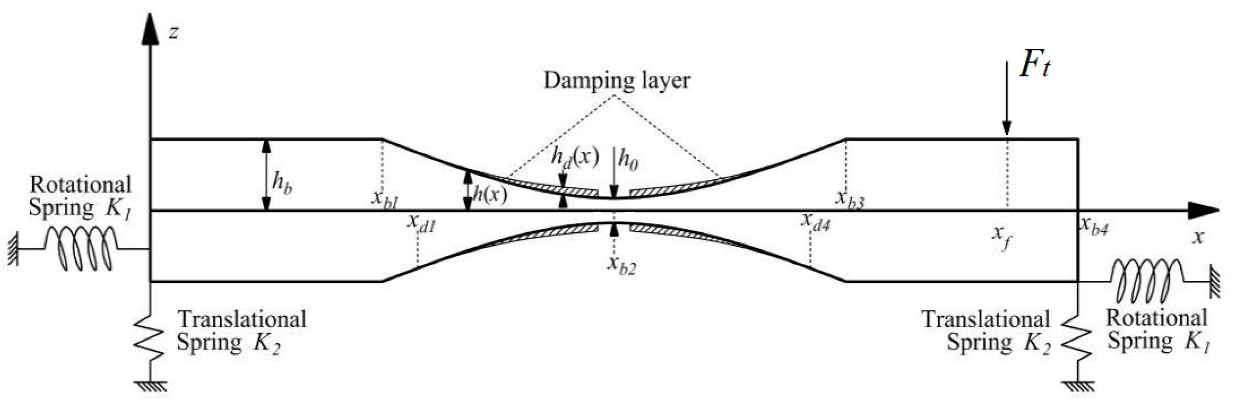
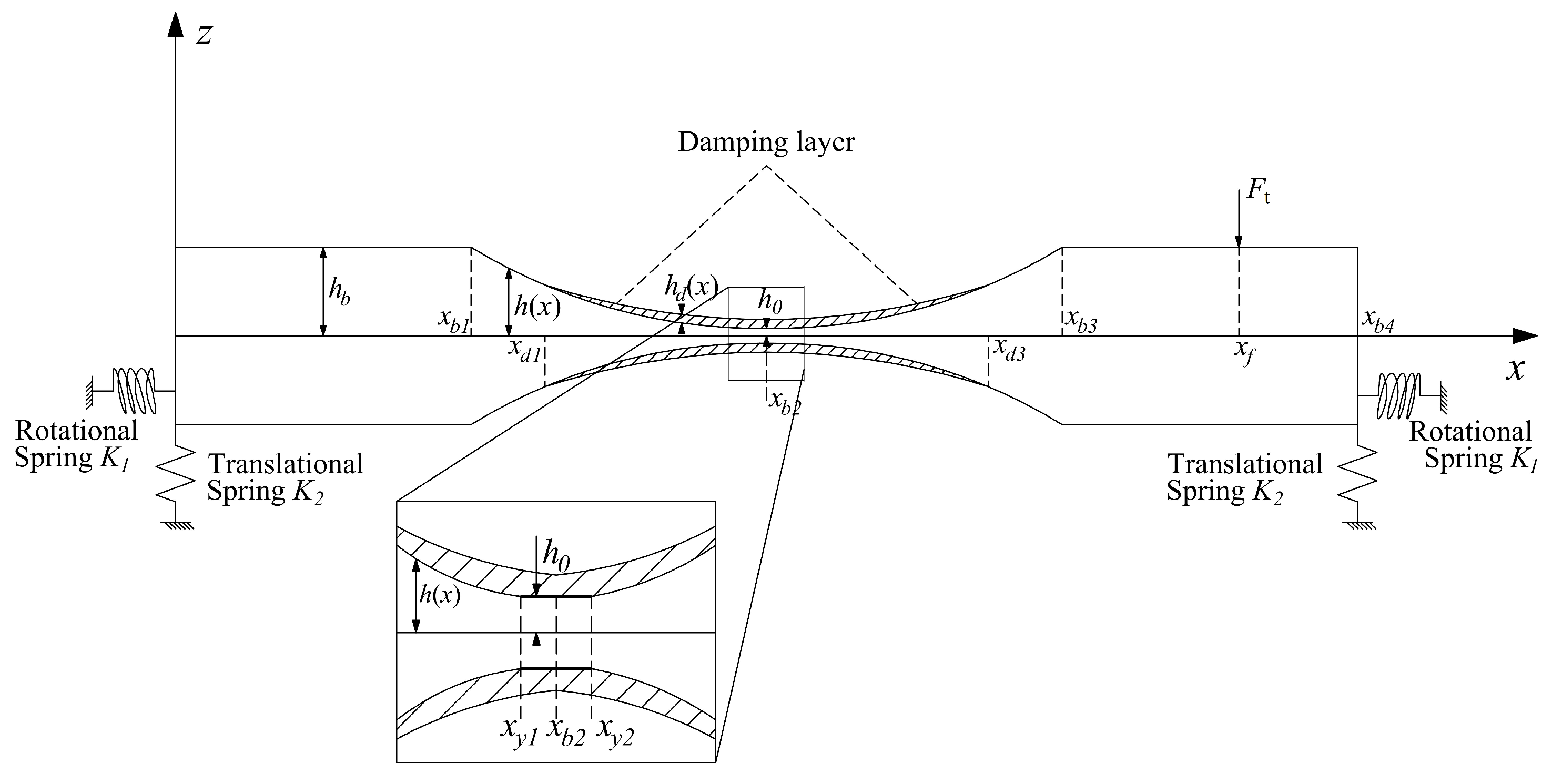
Referencing Figure 1, we examine a symmetric Euler–Bernoulli beam that experiences bending oscillations due to a localized force $F_t$ applied at position $x=x_f$. The beam’s structure includes a segment with a uniform thickness $h_b$ extending between $[0,x_{b1}]$ and $[x_{b3},x_{b4}]$, as well as a section with an ABH profile that features a thickness varying according to a power law from $x_{b1}$ to $x_{b3}$, i.e.,

$$h\left(x\right)=ϵ{(x-x_{b2})}^m+h_0,x\in [x_{b1},x_{b3}]$$

(1)

where $h_0$ is the thickness of the ABH structure at the location $x=x_{b2}$, $ϵ$ and m represent the slope and the ABH order, respectively. Both the lines $x=x_{b2}$ and $z=0$ are axes of symmetry for the structure in Figure 1. To enhance the wave trapping capability of the structure, damping material is affixed to both sides of the beam within the coordinates $[x_{d1},x_{d4}]$, with a thickness designated as $h_d\left(x\right)$. The beam’s edges are secured by a rotational spring with stiffness $K_1$ and a translational spring with stiffness $K_2$, and a variety of distinct boundary conditions are emulated by varying the values assigned to $K_1$ and $K_2$. The structure presented in Figure 1 usually is considered as a unit cell in a periodic ABH beam. Considering the inherent damping dissipation of the beam and the additional damping material, the complex modulus of elasticity can be articulated as follows:

$$E_{b,d}=E(1+i{\eta }_{b,d}),$$

(2)

where ${\eta }_{b,d}$ are the damping factors of the beam and the damping layers, respectively.

2.1. The Governing Equation

In this context, the displacement vector of the beam represents the movement along the x-axis and z-axis at every point along the beam, including the damping layer. It should be noted that the assumption presupposes an ideal adhesion between the damping layer and the primary beam, which is crucial for maintaining displacement continuity. $w(x,t)$ denotes the flexural displacement of any point on the beam in relation to time t. According to Euler–Bernoulli beam theory, the displacement field of the beam can be expressed as follows:

$$[-z{\displaystyle \frac{\partial w}{\partial x}},w].$$

(3)

Assume that $w(x,t)$ can be expanded as

$$w=\sum _k^n{a}_k\left(t\right){\phi }_k\left(x\right)={\mathbf{a}}^T\mathit{\phi },$$

(4)

where $\mathit{a}$ is a series of time-dependent coefficients to be determined and $\mathit{\phi }$ the admissible shape functions

$$\begin{array}{cc}\hfill & \mathit{a}\mathsf{(}\mathit{t}{\displaystyle \mathsf{)}}={[a_1\left(t\right),a_2\left(t\right),\cdots ,a_n\left(t\right)]}^T,\hfill \\ \hfill & \mathit{\phi }\mathsf{(}\mathit{x}\mathsf{)}={[{\phi }_1\left(x\right),{\phi }_2\left(x\right),\cdots ,{\phi }_n\left(x\right)]}^T.\hfill \end{array}$$

(5)

From classical Lagrange theory, the Lagrange quantity L for the system depicted in Figure 1 is given by

$$L=E_k-E_s+W,$$

(6)

where $E_k$ and $E_s$ are the kinetic energy and potential energy of the structure, respectively, and W is the work done on the ABH structure by external forces $F_t$,

$$E_k={\displaystyle \frac{1}{2}}\int {\rho }_b{\left({\displaystyle \frac{\partial w}{\partial t}}\right)}^{2}dV,$$

(7)

$$E_s={\displaystyle \frac{1}{2}}\int E_{b}I{\left({\displaystyle \frac{{\partial }^{2}w}{\partial x^2}}\right)}^{2}dx+E_e,$$

(8)

$$E_e={\displaystyle \frac{1}{2}}{K}_1[{\left({\displaystyle \frac{\partial w(x_{b4},t)}{\partial x}}\right)}^2+{\left({\displaystyle \frac{\partial w(0,t)}{\partial x}}\right)}^2]+{\displaystyle \frac{1}{2}}{K}_2[w^2(x_{b4},t)+w^2(0,t)],$$

(9)

$$W=F_{t}w(x_f,t),$$

(10)

where $E_e$ is the potential energy generated by the four springs at the boundary of the ABH beam, and ${\rho }_b$ and $E_{b}I$ are the density and the flexural rigidity of the beam, respectively. The integration process in Equations (7) and (8) must encompass both the beam and its associated damping layers. From [29], the damping layers are assumed to be fully integrated with the beam and are conceptualized as integral components of the system, characterized by their inherent material attributes, namely, the modulus of elasticity $E_d$ and the density ${\rho }_d$. Substituting Equations (4)–(10) into the Lagrange equation

$${\displaystyle \frac{d}{dt}}\left[{\displaystyle \frac{\partial L}{\partial \dot{\mathit{a}}\left(t\right)}}\right]-\left[{\displaystyle \frac{\partial L}{\partial \mathit{a}\left(t\right)}}\right]=0,$$

(11)

one can obtain the following governing equations of the ABH beam in matrix form:

$$\mathit{M}\ddot{\mathit{a}}\mathsf{(}\mathit{t}\mathsf{)}+\mathit{K}\mathit{a}\mathsf{(}\mathit{t}\mathsf{)}=\mathit{f}\mathsf{(}\mathit{t}\mathsf{)},$$

(12)

where $\mathit{M}$ and $\mathit{K}$ stand for the mass and stiffness matrices, $\mathit{f}\mathsf{(}\mathit{t}\mathsf{)}=F_t\mathit{\phi }\left(x_f\right)$ for the external force vector, and $\mathit{a}\mathsf{(}\mathit{t}\mathsf{)}$ for the response vector, as defined in Equation (5). The matrix $\mathit{M}$ can be broken down into three components that correspond to the uniformity (${\mathit{M}}_{\mathit{uni}}$), the ABH elements of the beam (${\mathit{M}}_{\mathit{ABH}}$), and the damping layers (${\mathit{M}}_{\mathit{d}}$), while the matrix $\mathit{K}$ can be dissected into four distinct segments, each associated with the aforementioned trio of components (${\mathit{K}}_{\mathit{uni}},{\mathit{K}}_{\mathit{ABH}},{\mathit{K}}_{\mathit{d}}$) as well as the springs (${\mathit{K}}_{\mathit{e}}$). The expressions of matrices $\mathit{M}$ and $\mathit{K}$ are given below:

$$\begin{array}{cc}\hfill \mathit{M}& =\int {\rho }_{b}A\left(x\right)\mathit{\phi }{\mathit{\phi }}^{T}dx={\mathit{M}}_{\mathit{uni}}+{\mathit{M}}_{\mathit{ABH}}+{\mathit{M}}_{\mathit{d}}\hfill \\ \hfill & =2[{\int }_0^{x_{b1}}{\rho }_b{h}_b\left(x\right)\mathit{\phi }{\mathit{\phi }}^{T}dx+{\int }_{x_{b1}}^{x_{b2}}{\rho }_{b}h\left(x\right)\mathit{\phi }{\mathit{\phi }}^{T}dx+{\int }_{x_{d1}}^{x_{d2}}{\rho }_d{h}_d\left(x\right)\mathit{\phi }{\mathit{\phi }}^{T}dx]\hfill \end{array}$$

(13)

$$\begin{array}{cc}\hfill \mathit{K}=& \int E_{b}I\left(x\right)\left({\displaystyle \frac{d^2\mathit{\phi }}{d{x}^2}}\right){\left({\displaystyle \frac{d^2\mathit{\phi }}{d{x}^2}}\right)}^{T}dx+{\mathit{K}}_{\mathit{e}}={\mathit{K}}_{\mathit{uni}}+{\mathit{K}}_{\mathit{ABH}}+{\mathit{K}}_{\mathit{d}}+{\mathit{K}}_{\mathit{e}}\hfill \\ \hfill =& {\displaystyle \frac{2}{3}}[{\int }_0^{x_{b1}}{E}_b{h}_b^3\left(x\right)\left({\displaystyle \frac{d^2\mathit{\phi }}{d{x}^2}}\right){\left({\displaystyle \frac{d^2\mathit{\phi }}{d{x}^2}}\right)}^{T}dx+{\int }_{x_{b1}}^{x_{b2}}{E}_b{h}_b^3\left(x\right)\left({\displaystyle \frac{d^2\mathit{\phi }}{d{x}^2}}\right){\left({\displaystyle \frac{d^2\mathit{\phi }}{d{x}^2}}\right)}^{T}dx]\hfill \\ \hfill & +{\displaystyle \frac{2}{3}}{\int }_{x_{d1}}^{x_{d2}}{E}_d[h_d^3\left(x\right)+3h_d^2\left(x\right)h\left(x\right)+3h_d\left(x\right)h^2\left(x\right)+h^3\left(x\right)]\left({\displaystyle \frac{d^2\mathit{\phi }}{d{x}^2}}\right){\left({\displaystyle \frac{d^2\mathit{\phi }}{d{x}^2}}\right)}^{T}dx\hfill \\ \hfill & +K_1\left({\displaystyle \frac{d^2\mathit{\phi }\mathsf{(}\mathbf{0}\mathsf{)}}{d{x}^2}}\right){\left({\displaystyle \frac{d^2\mathit{\phi }\mathsf{(}\mathbf{0}\mathsf{)}}{d{x}^2}}\right)}^T+K_2\mathit{\phi }\mathsf{(}\mathbf{0}\mathsf{)}\mathit{\phi }{\mathsf{(}\mathbf{0}\mathsf{)}}^T+K_1\left({\displaystyle \frac{d\mathit{\phi }\mathsf{(}{\mathit{x}}_{\mathit{b}\mathbf{4}}\mathsf{)}}{dx}}\right){\left({\displaystyle \frac{d\mathit{\phi }\mathsf{(}{\mathit{x}}_{\mathit{b}\mathbf{4}}\mathsf{)}}{dx}}\right)}^T\hfill \\ \hfill & +K_2\mathit{\phi }\mathsf{(}{\mathit{x}}_{\mathit{b}\mathbf{4}}\mathsf{)}\mathit{\phi }{\mathsf{(}{\mathit{x}}_{\mathit{b}\mathbf{4}}\mathsf{)}}^T\hfill \end{array}$$

(14)

2.2. The Solution of the Model Using the GEM

Given that the ABH beam is subjected to a harmonic external excitation with the circle frequency $\omega$, it follows that the structure’s steady-state response will also be harmonic. These can be mathematically represented as

$$\mathit{f}\mathsf{(}\mathit{t}\mathsf{)}=\mathit{F}{e}^{i\omega t},\mathit{F}=F_t·[{\phi }_1\left(x_f\right),\cdots ,{\phi }_n\left(x_f\right)],$$

(15)

$$\mathit{a}\mathsf{(}\mathit{t}\mathsf{)}=\mathit{A}{e}^{i\omega t},\mathit{A}=[a_1,a_2,\cdots ,a_n],$$

(16)

where $\mathit{F}$ represents the amplitude vector of the external force and $\mathit{A}$ the amplitude vector of the response. Substituting Equations (15) and (16) into Equation (12) yields

$$[\mathit{K}-{\omega }^2\mathit{M}]\mathit{A}=\mathit{F}.$$

(17)

When there is no external force applied, it translates into a generalized eigenvalue problem characterized by the presence of damped angular eigenfrequencies

$${\omega }_d^2={\omega }_n^2(1+i\eta )$$

(18)

where ${\omega }_n$ is the natural frequency of the system and $\eta$ denotes the modal loss factor, derived from the modal strain energy method (MSEM) [39], which employs a complex Young’s modulus, as detailed in Equation (2). The modal loss factor is the ratio of energy dissipated per cycle to the maximum energy stored within a cycle. It represents the viscoelastic properties of a material; a higher loss factor indicates greater viscosity, while a lower loss factor indicates greater elasticity. The modal loss factor plays a crucial role in evaluating how a structure dissipates energy when subjected to dynamic forces. It is especially valuable for determining the energy absorption capacity of damping layers due to the ABH effect.

The key to solving Equation (17) is to determine the shape functions in Equations (4) and (5). Research presented in [17,21,29] indicates that employing power series and polynomial expansions for shape functions may result in matrix singularities and poorly conditioned problems, thereby potentially reducing the solution’s accuracy. This is particularly relevant in the context of the ABH beam, where there are significant variations in wave numbers and wave velocities at the beam’s ends. The Gaussian function is proposed as the shape function due to its effectiveness in reducing the likelihood of singularities in the mass matrix calculations. The Gaussian function has the standard form below:

$$g\left(x\right)={\displaystyle \frac{1}{\sigma \sqrt{2\pi }}}exp\left(-{\displaystyle \frac{{(x-\mu )}^2}{2{\sigma }^2}}\right)$$

(19)

The function is symmetric with respect to the line $x=\mu$, and it reaches its peak at $x=\mu$. The value of $\sigma$ controls the width of the function. The larger the $\sigma$, the flatter the function and the more spread out the distribution; the smaller the $\sigma$, the sharper the function and the more concentrated the distribution. In this paper, we choose the following series of Gaussian functions as the shape functions:

$${\phi }_{i,k}\left(x\right)={\displaystyle \frac{1}{\sqrt{2\pi }}}{2}^{{\displaystyle \frac{a}{2}}}exp\left(-{\displaystyle \frac{{(2^{a}x-k)}^2}{2}}\right),$$

(20)

where the integer a serves as a scaling factor, while the integer k acts as a translation factor. By selecting appropriate values for a and k in Equation (20), the vibration of the entire ABH beam can be recovered [30]. a acts as a regulatory parameter that dictates the precision of the model. With an increasing number of recoverable modes as the value of a gets larger, the computational cost correspondingly rises. According to the suggestion in [30], we limit the range of k to $[-8,8]$ for the ABH beam considered in this paper. a is determined by the following relation:

$$a\ge ceil\left({log}_2\left({\displaystyle \frac{8}{x_{b4}}}\right)\right),$$

(21)

where $ceil\left(x\right)$ denotes the smallest integer that is greater than or equal to x. For every given a, the range of k is limited to

$$k\in [-4,ceil\left(2^a{x}_{b4}\right)+4]$$

(22)

2.3. Numerical FEM Validation

It is crucial to ascertain whether the GEM faithfully captures the deformation of a beam that incorporates a truncated ABH. This validation will be accomplished through comparative studies with FEM results within this subsection. The numerical simulation parameters for the ABH beam are specified in

Table 1. Parameters of the symmetric ABH structure.

Geometrical Parameters	Material Parameters
$x_{b1}=0.1$ m	Beam
$x_{b2}=0.2$ m	${\rho }_b$ = 7800 kg/m3
$x_{b3}=0.3$ m	$E_b$ = 210 GPa
$x_{b4}=0.4$ m	${\eta }_b=0.005$
$x_f=0.35$ m	Damping layer
$ϵ$ = 0.5 m−1,  m = 2	${\rho }_d$ = 950 kg/m3
$h_0=0.0002$ m	$E_d$ = 5 GPa
$h_b=0.0052$ m	${\eta }_d=0.3$

.

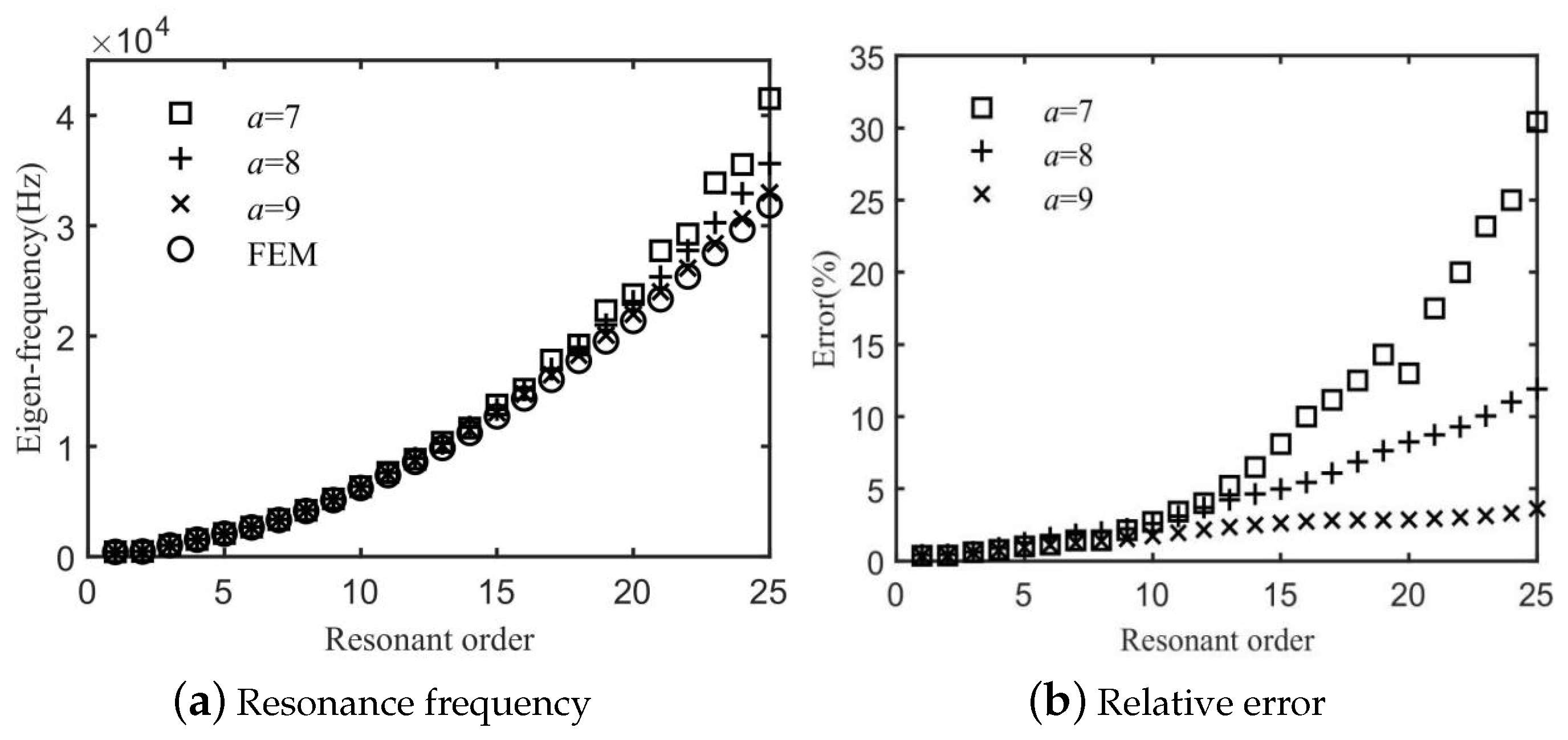
The eigenfrequencies and eigenvectors of the ABH beam are determined utilizing two distinct approaches: the first employs the GEM in conjunction with Equation (17), while the second approach relies on a 2D planar finite element model that encompasses 19,204 elements, all within the COMSOL software environment. Figure 2 illustrates a comparative analysis of the first 25 eigenvalues obtained from both the GEM and FEM, with the scaling factor (as defined in Equation (20)) taken as $a=7,8,9$, respectively. It is evident that the GEM results quickly align with the FEM results as the value of a increases. As depicted in Figure 2b, selecting $a=9$ results in a residual discrepancy of approximately $3\%$ for the first 25 resonant sequences. Figure 3 displays the modal shapes corresponding to various resonant frequencies, as determined by the FEM and GEM outlined in this study. The results indicate that the analytical model using the GEM is capable of accurately capturing the substantial deformations at the tip of the ABH beam.

3. Analysis of Damping Layer Parameters

In this section, we analyze the impact of the damping layer’s parameters, such as position, thickness, and shape, on the system’s energy dissipation efficiency, characterized by the modal loss factor as defined by Equation (18), using the semi-analytical solutions obtained from the GEM.

3.1. The Effect of the Damping Layer’s Position

We fix the thickness of the damping layer at $h_d=0.0002m$, and consider four different scenarios of adhesive attachment positions:

$$\begin{array}{cc}\hfill & Case1:x_{d1}=0.14m,x_{d4}=0.26m,\hfill \\ \hfill & Case2:x_{d1}=0.15m,x_{d4}=0.25m,\hfill \\ \hfill & Case3:x_{d1}=0.16m,x_{d4}=0.24m,\hfill \\ \hfill & Case4:x_{d1}=0.18m,x_{d4}=0.22m.\hfill \end{array}$$

(23)

Other parameter values of the damping layers continue to utilize those listed in Table 1. Figure 4 illustrates the effect of various placements of damping layers on the modal loss factor. It can be observed from Figure 4 that although Case 1 has the longest adhesive length, the variation in the system’s damping coefficient is not pronounced compared to other adhesive lengths. As the mode shape order increases, the impact of different adhesive lengths gradually converges. This suggests that the adhesive length has a minimal influence on the ABH effect in this case and can be disregarded.

3.2. The Effect of the Damping Layer’s Thickness ($h_d$ Remains Unchanged)

Consider that the position of the damping layer is confined between $x_{d1}=0.14m$ and $x_{d4}=0.26m$, and the thickness is taken as $h_d=0.0002m$, $0.0005m$, $0.001m$, $0.005m$, respectively. The comparative outcomes are depicted in Figure 5. An examination of Figure 5 reveals that for low-order modes, the modal loss factor is very sensitive to the thickness of the damping layer, with the maximum increase in the modal loss factor being 16 times when the thickness is increased by 25 times. As the order of the vibration mode increases, the increase in the modal loss factor caused by the increase in damping layer thickness will exhibit a more pronounced fluctuation phenomenon. This indicates that increasing the thickness of the damping layer does not always enhance system performance. When the damping layer becomes too thick to the point where it significantly affects the mass and stiffness of the truncated section, it may actually have an adverse effect by resonating with a specific order of frequency.

3.3. The Effect of the Damping Layer’s Thickness ($h_d$ Is Variable)

In this subsection, the impact of the damping layer thickness distribution on the overall system damping is explored through the establishment of various functions representing changes in damping layer thickness. The damping layer is positioned within the range $[x_{d1},x_{d4}]=[0.14,0.26]$. For ease of comparison, the effect of a damping layer with a constant thickness of $0.0002m$ is used as the reference. The thickness of the damping layer, $h_d$, is considered as a function of x. For the sake of comparison, two restrictions for $h_d\left(x\right)$ are assumed as follows:

• The mass of the damping layer remains constant during the variation in $h_d\left(x\right)$:

  $${\int }_{x_{d1}}^{x_{d4}}{h}_d\left(x\right)dx={\int }_{x_{d1}}^{x_{d4}}0.0002dx$$

  (24)
• The thickness variation function $h_d\left(x\right)$ is symmetric about $x=x_{b2}$, and it satisfies

  $$h_d\left(x_{b2}\right)=0,or{h}_d\left(x_{d1}\right)=h_d\left(x_{d4}\right)=0.$$

  (25)

3.3.1. Case of $h_d\left(x_{b2}\right)=0$

The thickness $h_d\left(x\right)$ varies according to the following different functional patterns:

$$\begin{array}{cc}\hfill & h_{d1}\left(x\right)={\displaystyle \frac{1}{150}}|x-0.2|,\hfill \\ \hfill & h_{d2}\left(x\right)=-{\displaystyle \frac{1}{36}}{\left(\right|x-0.2|-0.14)}^2+{\displaystyle \frac{49}{90000}},\hfill \\ \hfill & h_{d3}\left(x\right)=-{\displaystyle \frac{1}{12}}{\left(\right|x-0.2|-0.06)}^2+{\displaystyle \frac{3}{10000}},\hfill \\ \hfill & h_{d4}\left(x\right)={\displaystyle \frac{100}{27}}{|x-0.2|}^3,x\in [0.14,0.26]\hfill \end{array}$$

(26)

The graphs of functions in Equation (26) are illustrated in Figure 6. Figure 7 demonstrates how different functions, $h_d\left(x\right)=h_{d1},\cdots ,h_{d4}$, respectively, for varying the thickness of the damping layer affect the modal loss factor. From Figure 7, it is observed that positioning the damping layer’s maximum thickness away from the ABH tip results in a less effective enhancement of the ABH effect compared to a damping layer with uniform thickness. The damping layer that varies in thickness according to the function $h_{d3}$ shows the most pronounced effect in enhancing the ABH effect, followed by the functions $h_{d1}$ and $h_{d2}$, with the least effective being the variation according to the function $h_{d4}$. Figure 7 demonstrates that the choice of damping layer thickness variation function has a very significant impact on the ABH effect.

3.3.2. Case of $h_d\left(x_{d1}\right)=h_d\left(x_{d4}\right)=0$

Consider that the thickness $h_d\left(x\right)$ fluctuates in accordance with several distinct functional forms:

$$\begin{array}{cc}\hfill & h_{d5}\left(x\right)=-{\displaystyle \frac{1}{150}}|x-0.2|+{\displaystyle \frac{1}{2500}},\hfill \\ \hfill & h_{d6}\left(x\right)=-{\displaystyle \frac{1}{12}}{(x-0.2)}^2+{\displaystyle \frac{3}{10000}},\hfill \\ \hfill & h_{d7}\left(x\right)={\displaystyle \frac{1}{6}}{\left(\right|x-0.2|-0.06)}^2,\hfill \\ \hfill & h_{d8}\left(x\right)=-{\displaystyle \frac{100}{81}}{|x-0.2|}^3+{\displaystyle \frac{1}{3750}},x\in [0.14,0.26]\hfill \end{array}$$

(27)

The plots of the functions given in Equation (27) are depicted in Figure 8. Figure 9 illustrates the improvement in the ABH effect achieved through various thickness variation functions, with the damping layer’s maximum thickness positioned at the ABH tip. Varying the damping layer’s thickness based on the functions $h_{d5}$ through $h_{d8}$ achieves better outcomes than maintaining a constant thickness throughout. This demonstrates that a uniform application of damping material across the entire region $[x_{d1},x_{d4}]$ is not optimal. With a fixed total amount of damping material, concentrating more damping at the ABH tip and tapering off as we move away from it leads to a markedly improved performance over a uniform distribution. Figure 9 shows that among the different thickness variation functions, the ABH effect is most significant when the thickness of the damping layer is adjusted according to the function $h_{d7}\left(x\right)$. The findings from this subsection reveal that selecting the appropriate thickness variation function for the damping layer has a substantial influence on the ABH effect, warranting further investigation into optimizing the shape of the function.

4. Optimization of the Damping Layer’s Position and Thickness

From the analysis in the previous section, we consider that the thickness of the damping layer varies as follows:

$$h_d\left(x\right)=c_1\left(\right|x-c_0{|+c_2)}^n+c_3,$$

(28)

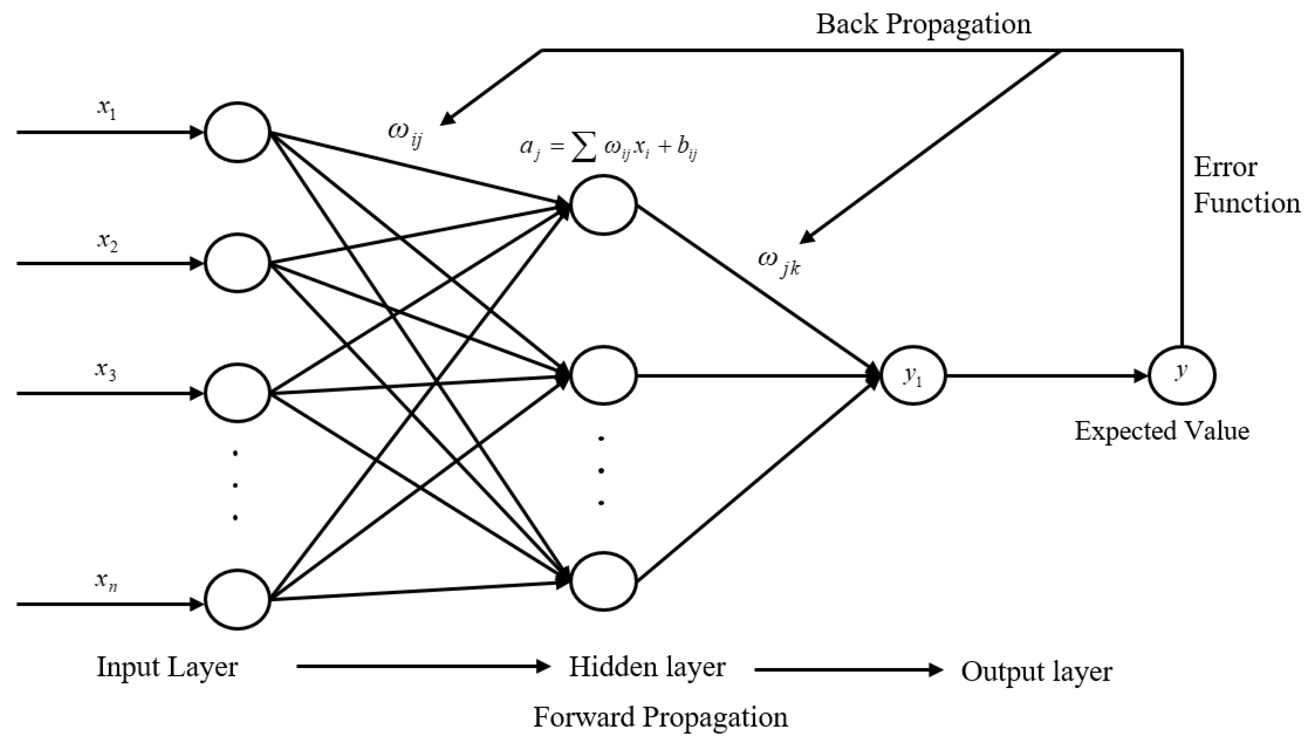
where $c_{0,1,2,3}$ and n are the parameters that need to be optimized for determining the best damping layer thickness variation function under conditions (24) and (25). In this section, we will find the optimal form of the damping layer thickness variation function based on BP neural networks. BP neural networks are a class of artificial neural networks that are widely used for various tasks such as pattern recognition, prediction, and data classification. A BP neural network typically consists of an input layer, one or more hidden layers, and an output layer. Each layer is composed of a set of neurons, and each neuron is connected to the neurons in the next layer through weights. A typical BP neural network structure is shown in Figure 10.

When a training example is presented, the input is passed through the network. Each neuron in the hidden layers computes a weighted sum of its inputs and applies an activation function to it. The activation function introduces nonlinearity into the model, allowing it to learn complex relationships. Common activation functions used in BP neural networks include the Sigmoid function, hyperbolic tangent (tanh), and the rectified linear unit (ReLU). The choice of activation function can have a significant impact on the network’s performance. After the forward pass, the network’s prediction is compared to the actual target value, and the error is calculated. The choice of loss function depends on the specific task. Common loss functions include mean squared error for regression tasks and cross-entropy loss for classification tasks. This error is then propagated back through the network, adjusting the weights to minimize the error. The process involves the calculation of gradients using the chain rule of calculus. The learning in a BP neural network is achieved through iterative training. During each iteration, the network processes a batch of training data, calculates the error, and updates the weights. This process is repeated over many epochs until the network’s performance on a validation set is satisfactory.

The parameters $c_{0,1,2,3}$ and n in Equation (28) and the position of the damping layer $[x_{d1},x_{d4}]$ are used as six different indicator inputs for the BP neural network. The values of the output layer represent the desired results of the prediction, signifying the functional purpose that the network aims to achieve. In this model, the damping coefficients of the system at different vibration orders need to be predicted. Considering the practical needs of engineering, this paper predicts the damping coefficients for the first ten orders of the system; hence, the number of nodes in the output layer is 10. We set up two hidden layers through the design of network architecture, cross-validation, and performance evaluation. Determining the appropriate number of neurons in each hidden layer is crucial for neural network design. Insufficient neurons may result in underfitting, preventing the network from capturing the full complexity of the training data and thus weakening its predictive capabilities. Conversely, an excess of neurons can cause overfitting, where the network performs well on training data but poorly on unseen data, and also prolongs the training process. For networks with multiple hidden layers, the number of nodes in the hidden layers can be determined using the following empirical formula:

$$m=\sqrt{n+l}+\alpha ,m=\sqrt{nl},$$

(29)

where the number of nodes in the hidden layer is denoted by m, the number of nodes in the input layer by n, and the number of nodes in the output layer by l. The constant $\alpha$ is greater than 1 and less than 10. According to the empirical formula, this paper sets the number of hidden layer nodes to be eight and nine, respectively. Considering that the output value of the Sigmoid function ranges from 0 to 1, and the derivative ranges from 0 to 0.25, it can conveniently control the magnitude of weight updates during the backpropagation process and avoid the problem of gradient vanishing. The choice of activation function is the Sigmoid function.

When seeking the minimum value of the error function, the Levenberg–Marquardt algorithm [40] is used for iteration. The algorithm is an improved method that lies between the Gauss–Newton method and the gradient descent method [41]. The algorithm incorporates a step-size adjustment parameter. In situations where the error function decreases sharply in the direction of the gradient, a reduced step-size factor is applied, thereby aligning the method more closely with the Gauss–Newton approach. Conversely, when the descent is slower, a larger step-size factor is used, making the algorithm more similar to the gradient descent method.

We set the following range for the six input parameters separately,

$$\begin{array}{cc}\hfill & c_0\in [0,0.2],c_1\in [-2,2],c_2\in [-0.06,0]\hfill \\ \hfill & c_3\in [0,0.005],n\in [0,3],[x_{d1},x_{d4}]\subseteq [0.1,0.3],\hfill \end{array}$$

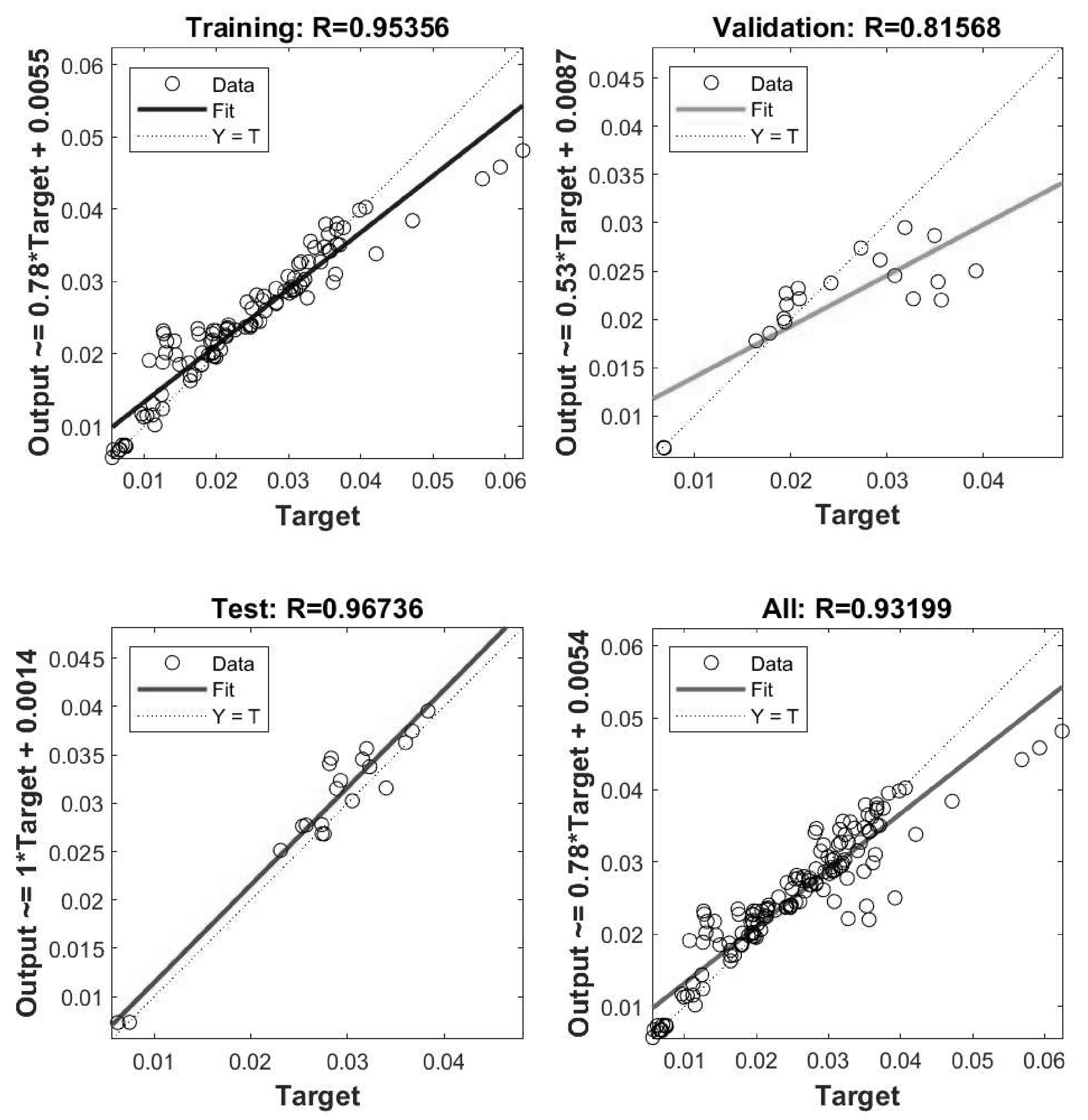
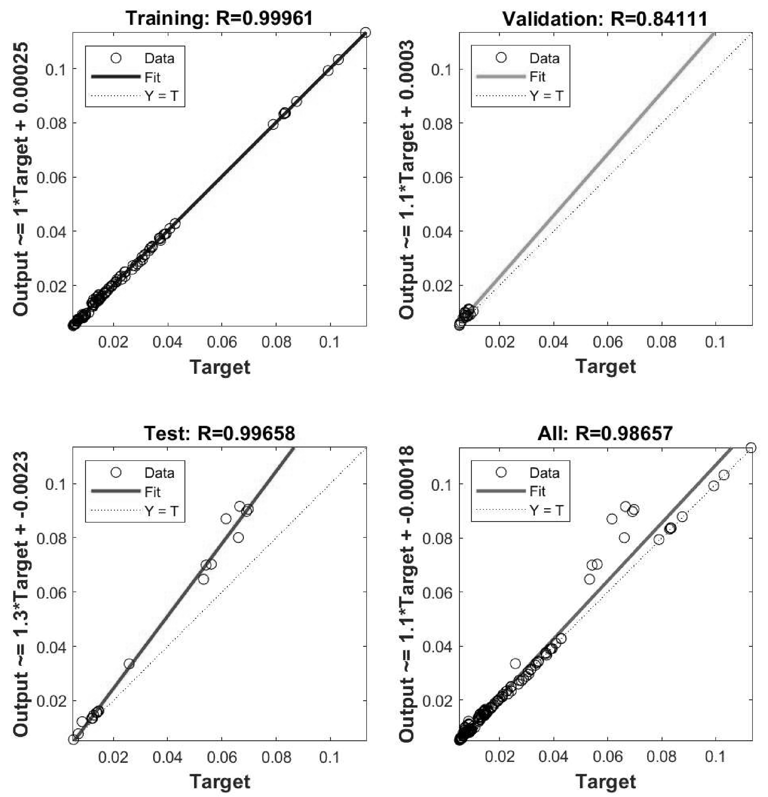
and use the larger mean of output data and the smaller variance as the evaluation criteria. The training samples and validation samples both originate from theoretical computational results. Figure 11 illustrates the degree of fit of the BP network after being trained with Matlab software. It is evident that the linear correlation between the output data of the BP model and the training, validation, and test datasets exceeds 0.84 in each case. The overall fit rate of the entire model is 0.98657, indicating a high degree of fit, making the model acceptable and suitable as a predictive network model. The optimal damping layer thickness variation function predicted by the BP network is

$$h_{dp}\left(x\right)={\displaystyle \frac{4}{3}}{\left(\right|x-0.2|-0.03)}^2,x\in [0.17,0.23]$$

(30)

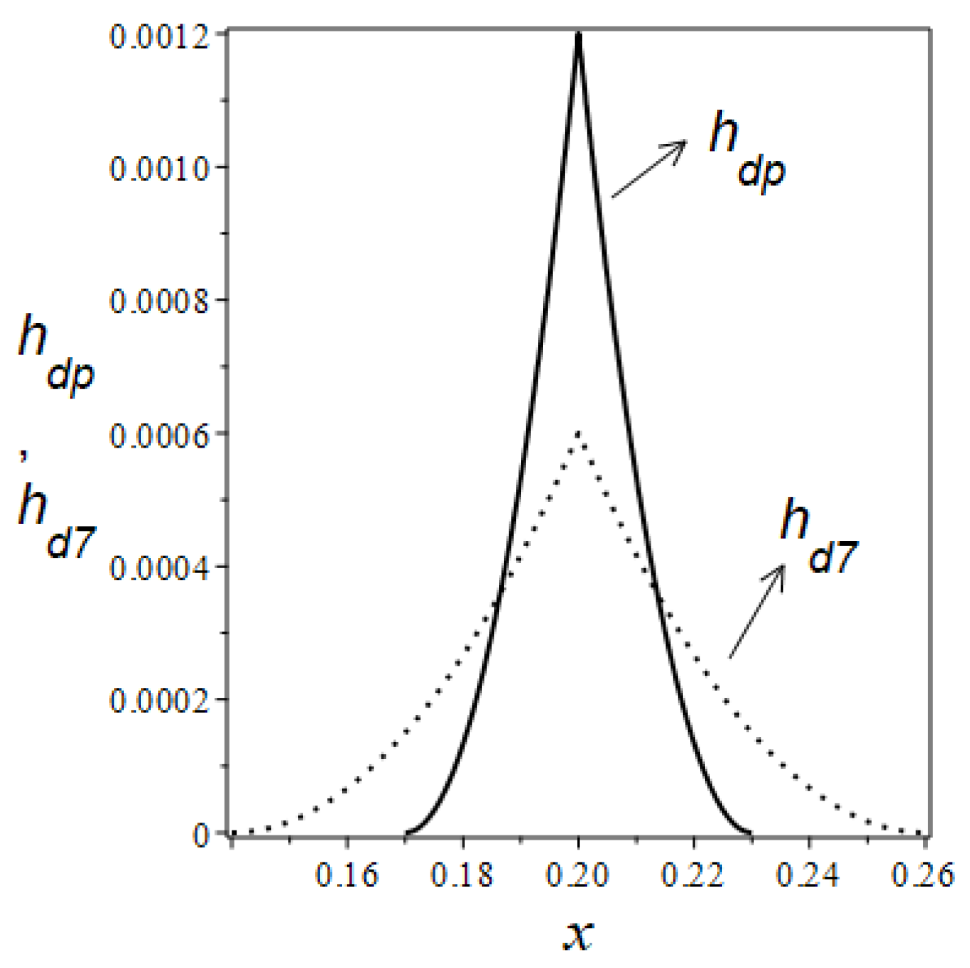
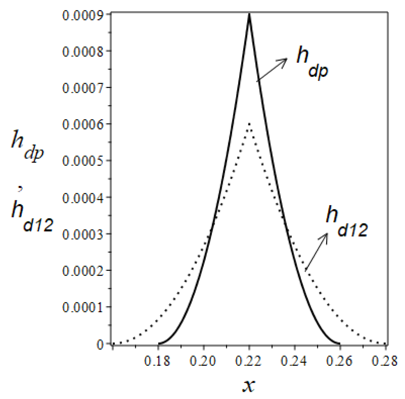
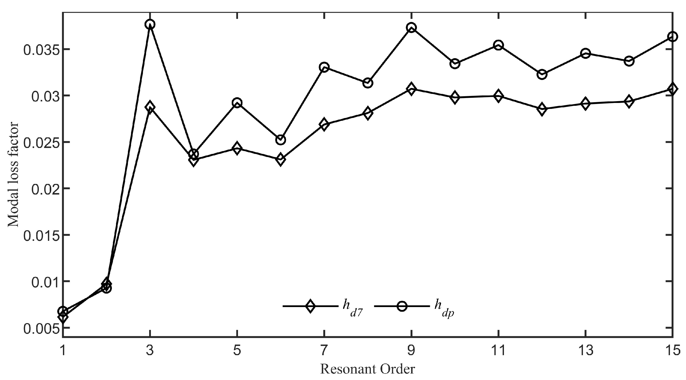
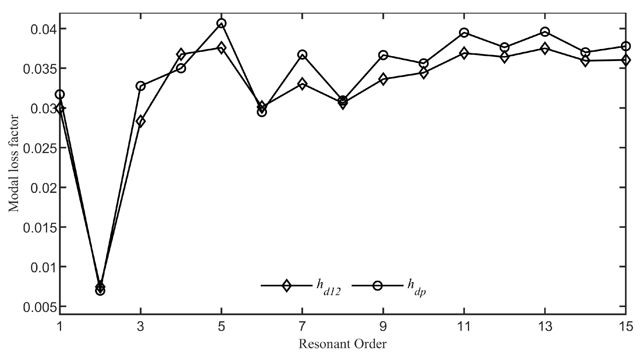
Figure 12 displays the graphical representations of the functions $h_{dp}$, as defined by Equation (30), and $h_{d7}$, as defined by Equation (27). The comparison of the effect of different damping layer thicknesses (varying according to the functions $h_{dp}$ and $h_{d7}$) on the ABH effect is shown in Figure 13. It is clear that as the resonance order increases, the modal loss factors of the system with damping layer thickness set according to the function $h_{d7}$ gradually stabilize around 0.029, whereas with the damping layer thickness set according to the function $h_{dp}$, the modal loss factors gradually stabilize around 0.035. The average value of the modal loss factors for the first fifteen modes of the system with damping layer thickness set according to the function $h_{d7}$ is 0.0252, while for the function $h_{dp}$ it is 0.0293, representing an approximate $16.2\%$ increase compared to the $h_{d7}$ scenario. Figure 13 shows the effectiveness of optimization using the BP neural network.

The analysis based on BP neural network optimization indicates that to achieve a good ABH effect, it is not necessary to apply the damping layer over the entire ABH section. The thickness of the damping layer should be maximized at the ABH tip, with a swift reduction as one moves away from the tip. Additionally, it is unnecessary to apply a damping layer in regions that are distant from the tip.

Given that the thickness of the damping layer significantly affects the vibration reduction performance of the system, precise control over the damping layer thickness on the ABH beam is essential in practical applications. To further elucidate the impact of the damping layer thickness tolerances on the ABH effect, we consider the damping layer thickness varying according to the following two functions:

$$\begin{array}{cc}\hfill & h_{dpa}\left(x\right)={\displaystyle \frac{4}{3}}{\left(\right|x-0.2|-0.031)}^2,\hfill \\ \hfill & h_{dps}\left(x\right)={\displaystyle \frac{4}{3}}{\left(\right|x-0.2|-0.029)}^2,x\in [0.17,0.23].\hfill \end{array}$$

(31)

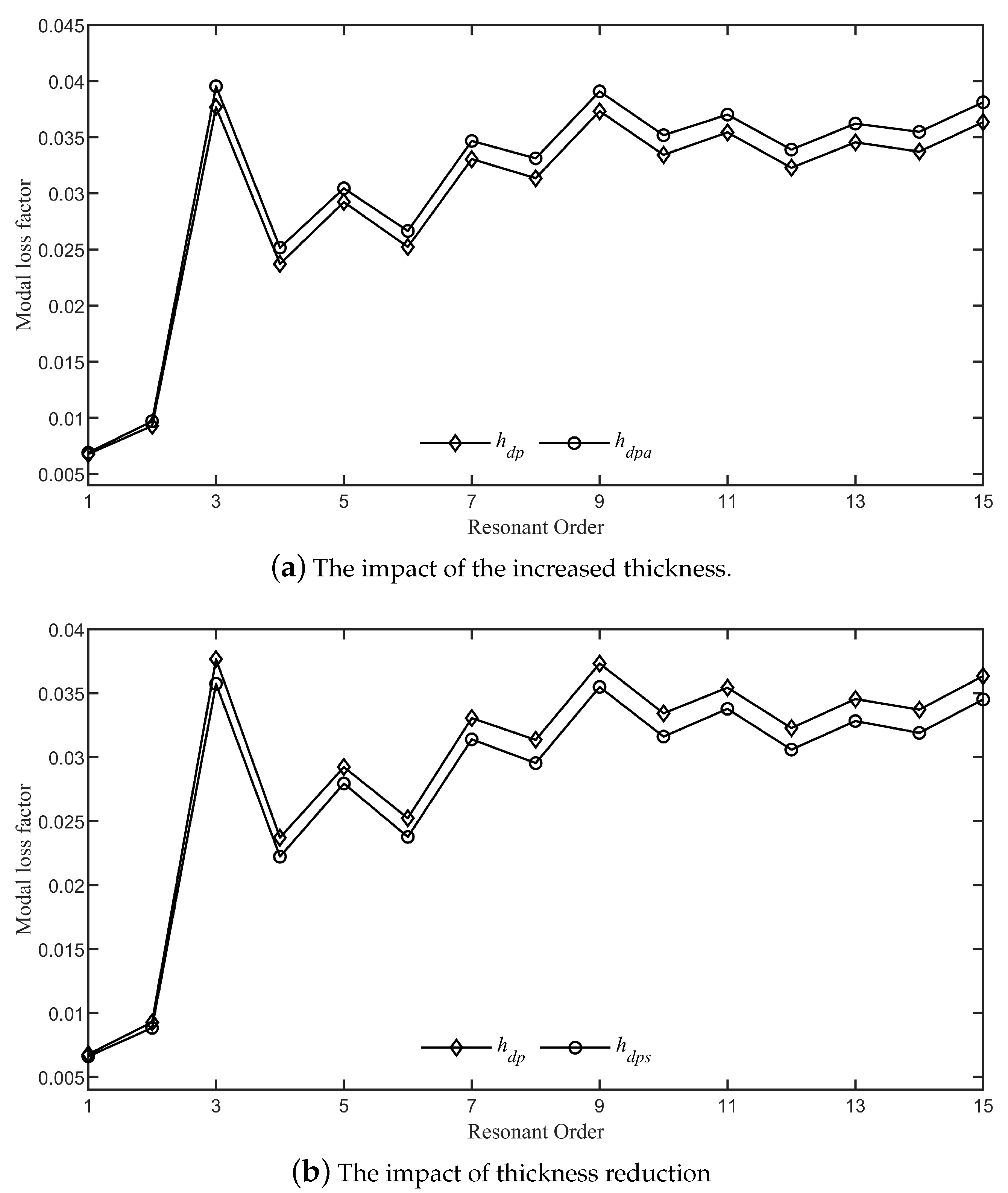
The two functions above are employed to simulate the manufacturing tolerances that arise in the optimized function $h_{dp}\left(x\right)$, presented in Equation (30). The impact of manufacturing tolerances in the damping layer thickness on the ABH effect is illustrated in Figure 14.

As can be seen from Figure 14, when the optimized shape of the thickness does not undergo significant changes, minor manufacturing tolerances in the damping layer thickness only cause minor variations in the system’s vibration reduction performance. When the damping layer thickness is slightly increased, the system’s vibration reduction performance is also slightly enhanced, and vice versa. This indicates that optimizing the thickness profile of the damping layer is feasible in practical applications.

To achieve more precise control over the thickness of the damping layer in actual manufacturing, the following strategies and methods can be considered [42,43]: Firstly, the thickness of damping materials can be controlled through optimized design. For instance, the surface of the structure can be divided into multiple zones, with the thickness of the damping material in each zone treated as a design variable for optimization. This approach allows the damping layer to meet specific requirements for vibration reduction. Secondly, the performance of damping materials can be enhanced through methods such as blending and copolymerization. These techniques help minimize tolerance issues arising from material inhomogeneity. Additionally, a multi-layer structural design can be employed, with the overall thickness uniformity controlled by adjusting the thickness and number of layers. Moreover, to maximize the effectiveness of the damping layer, the bonding area of the damping material should be as extensive as possible. Considering the entire construction process, a bonding area exceeding $80\%$ can serve as a process indicator to ensure the quality of damping material installation.

5. Further Discussion

In this section, we examine the alterations made to the ABH beam illustrated in Figure 1, which are detailed in Figure 15. The beam comprises three distinct segments: The initial segment extends across the intervals $[0,x_{b1}]$ and $[x_{b3},x_{b4}]$, with a consistent thickness of $h_b$. The second segment, which spans $[x_{y1},x_{y2}]$, maintains a uniform thickness of $h_0$. The third segment features an ABH profile, with its thickness varying according to a power law between the points $x_{b1}$ and $x_{y1}$, as well as between $x_{y2}$ and $x_{b3}$. The thickness variation of the beam can be expressed as follows:

$$h\left(x\right)=\left\{\begin{array}{cc}ϵ{(x-x_{y1})}^m+h_0,\hfill & \hfill x\in [x_{b1},x_{y1}]\\ h_0,\hfill & \hfill x\in [x_{y1},x_{y2}]\\ ϵ{(x-x_{y2})}^m+h_0,\hfill & \hfill x\in [x_{y2},x_{b3}]\end{array}\right.$$

(32)

where $ϵ$ and m represent the slope and the ABH order, respectively. The structure depicted in Figure 15 exhibits symmetry about both the line $x=x_{b2}$ and the plane $z=0$. Damping material is attached to both flanges of the beam, spanning the region $[x_{d1},x_{d3}]$, with a variable thickness denoted by $h_d\left(x\right)$. The beam’s ends are supported by rotational springs of stiffness $K_1$ and translational springs of stiffness $K_2$, allowing for a range of boundary conditions to be simulated by adjusting the values of $K_1$ and $K_2$. The parameters for the modified ABH beam are given in

Table 2. Parameters of the modified symmetric ABH structure.

Geometrical Parameters	Material Parameters
$x_{b1}=0.1$ m	Beam
$x_{b2}=0.22$ m	${\rho }_b$ = 7800 kg/m3
$x_{b3}=0.34$ m	$E_b=$ 210 Gpa
$x_{b4}=0.44$ m	${\eta }_b=0.005$
$x_f=0.39$ m	Damping layer
$ϵ$ = 0.5 m−1, $m=2$	${\rho }_d$ = 950  kg/m3
$x_{y1}=0.2$ m, $x_{y2}=0.24$ m	$E_d=$ 5 Gpa
$h_0=0.0002,h_b=0.0052$ m	${\eta }_d=0.3$

. The difference between Figure 1 and Figure 15 is that the structure in Figure 15 includes an additional segment in $[x_{y1},x_{y2}]$, where the beam’s thickness remains constant at $h_0$. In this section, we focus on discussing the impact of adding a segment with constant thickness $h_0$ on the system’s ABH effect over the interval $[x_{y1},x_{y2}]$.

5.1. the Effect of the Damping Layer’s Position

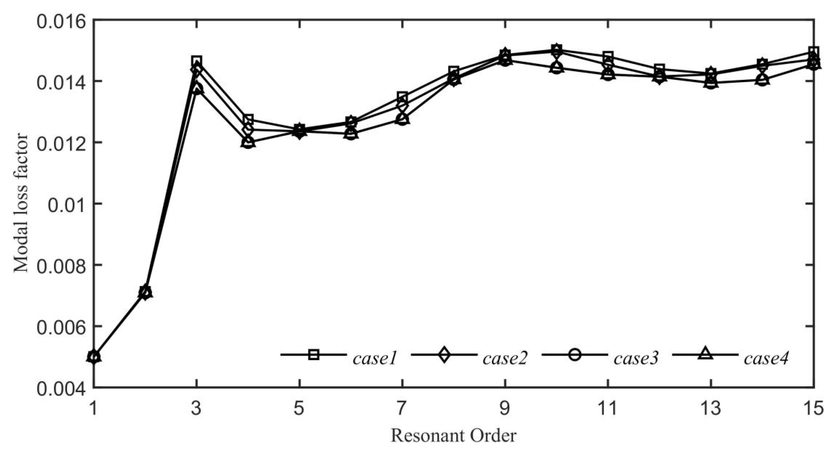
We set the thickness of the damping layer to a constant value of $h_d=0.0002m$ and explore four distinct scenarios regarding the placement of adhesive bonds:

$$\begin{array}{cc}\hfill & Case1:x_{d1}=0.18m,x_{d3}=0.26m,\hfill \\ \hfill & Case2:x_{d1}=0.16m,x_{d3}=0.28m,\hfill \\ \hfill & Case3:x_{d1}=0.14m,x_{d3}=0.3m,\hfill \\ \hfill & Case4:x_{d1}=0.12m,x_{d3}=0.32m.\hfill \end{array}$$

(33)

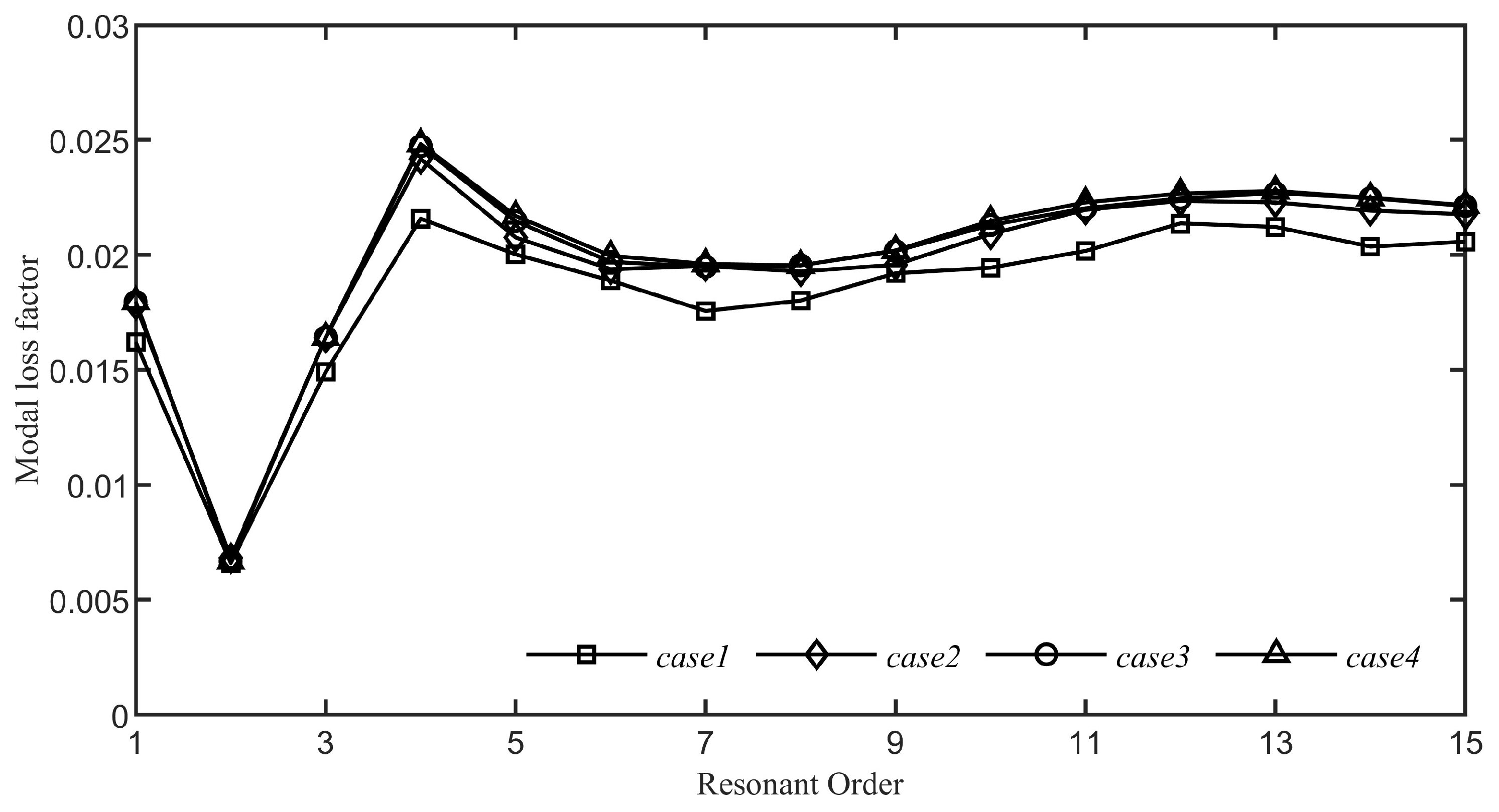
Figure 16 illustrates the effects of different damping layer configurations on the modal loss factor. As shown in Figure 16, even though Case 4 has the longest adhesive length, the changes in the modal loss factor of the system are not markedly different from those with shorter adhesive lengths. As the mode shape order increases, the impact of varying adhesive lengths becomes less pronounced. This suggests that the length of the adhesive has a minimal effect on the ABH effect in this context and can be considered insignificant.

5.2. The Effect of the Damping Layer’s Thickness ($h_d$ Is Variable)

In this subsection, we delve into the influence of the distribution of damping layer thickness on the system’s overall damping by defining several functions that model variations in damping layer thickness under the conditions specified by Equations (24) and (25). The damping layer is situated within $[x_{d1},x_{d3}]=[0.16,0.28]$. Additionally, the impact of a damping layer with a uniform thickness of $0.0002m$ serves as a benchmark for comparison. 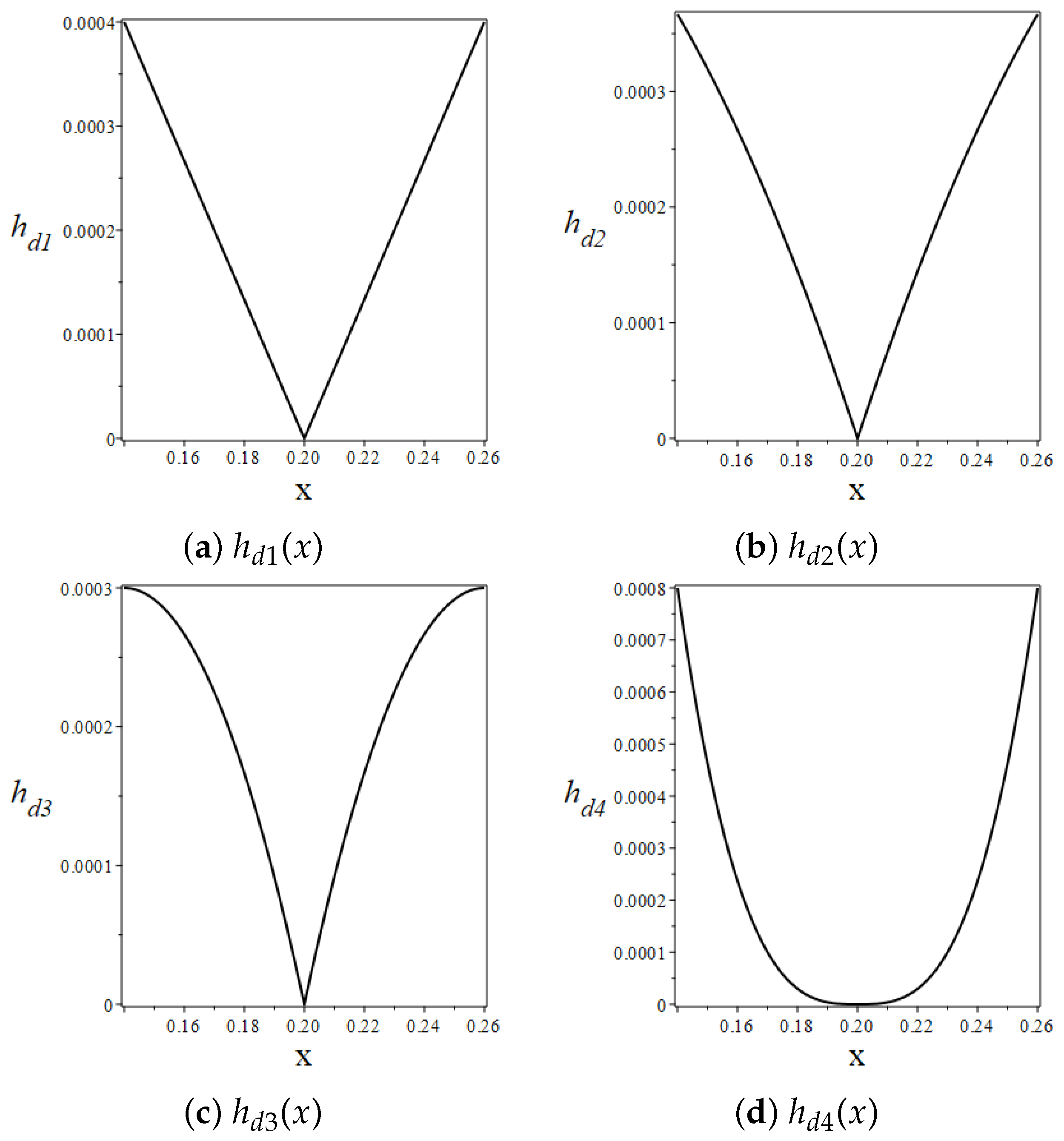Following the findings from Section 3, which suggest that increased damping at the ABH tip yields better outcomes, we now contemplate the thickness $h_d\left(x\right)$ that alters according to various specific mathematical expressions:

$$\begin{array}{cc}\hfill & h_{d10}\left(x\right)=-{\displaystyle \frac{1}{150}}|x-0.22|+{\displaystyle \frac{1}{2500}},\hfill \\ \hfill & h_{d11}\left(x\right)=-{\displaystyle \frac{1}{12}}{(x-0.22)}^2+{\displaystyle \frac{3}{10000}},\hfill \\ \hfill & h_{d12}\left(x\right)={\displaystyle \frac{1}{6}}{\left(\right|x-0.22|-0.06)}^2,\hfill \\ \hfill & h_{d13}\left(x\right)=-{\displaystyle \frac{100}{81}}{|x-0.22|}^3+{\displaystyle \frac{1}{3750}},x\in [0.16,0.28]\hfill \end{array}$$

(34)

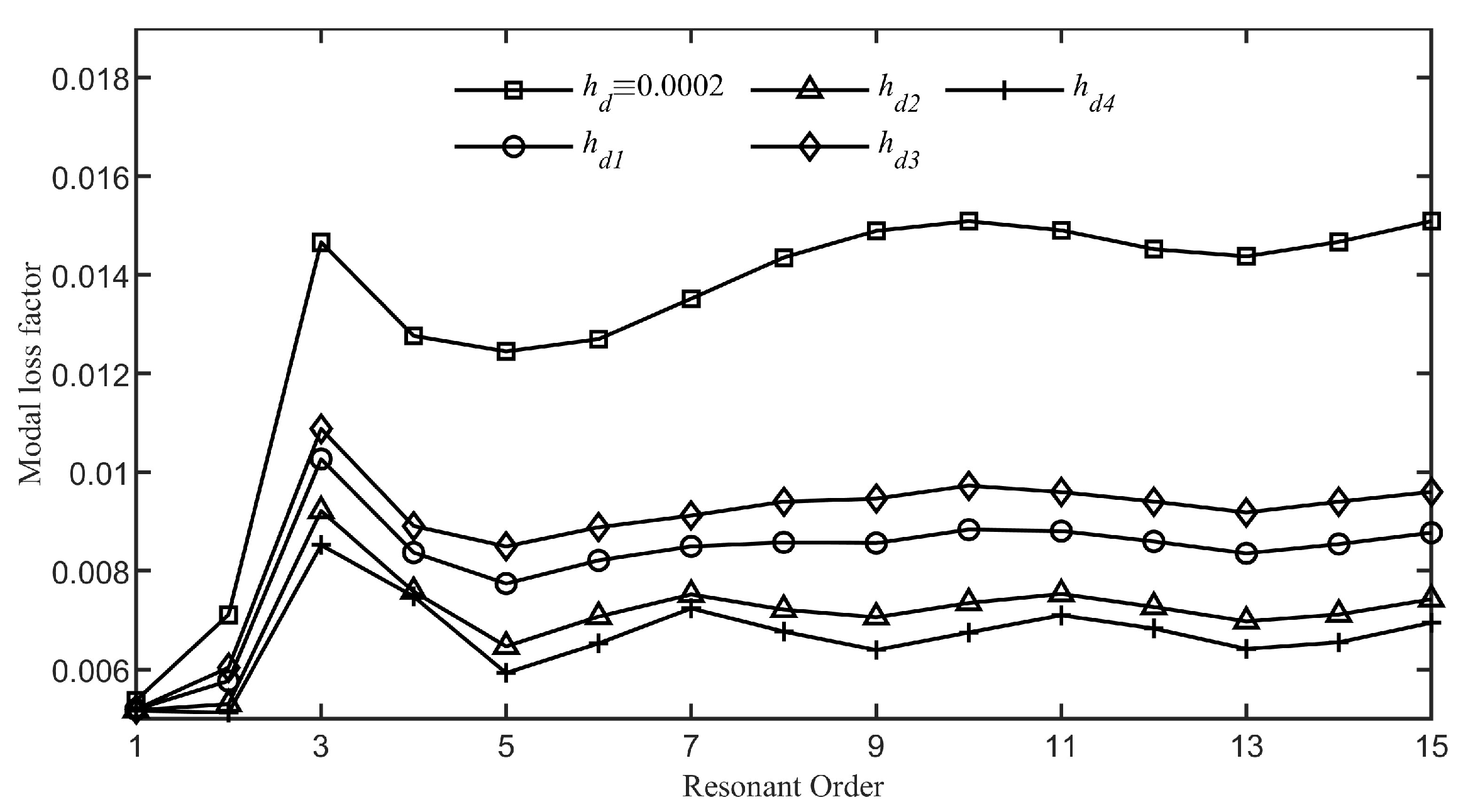
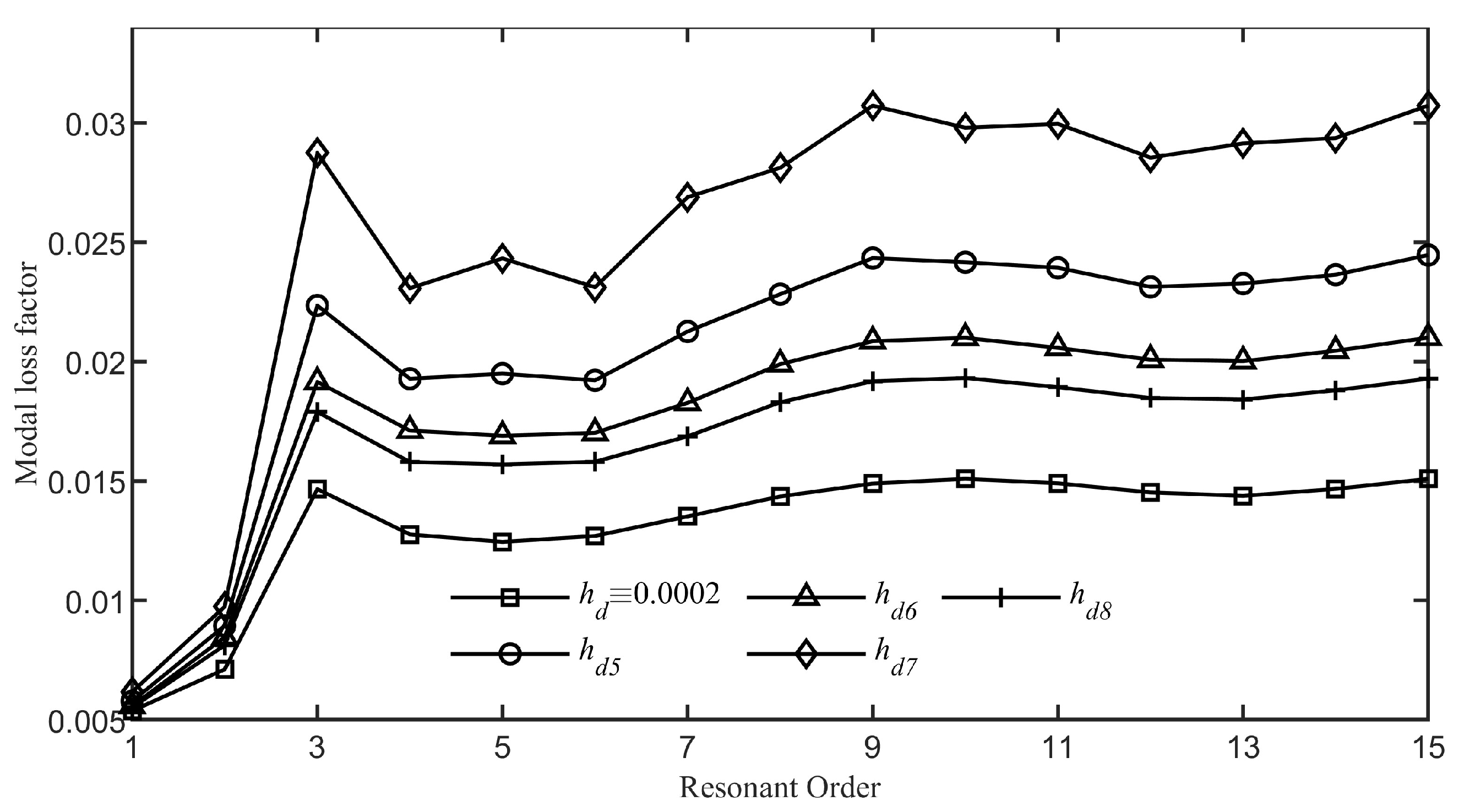
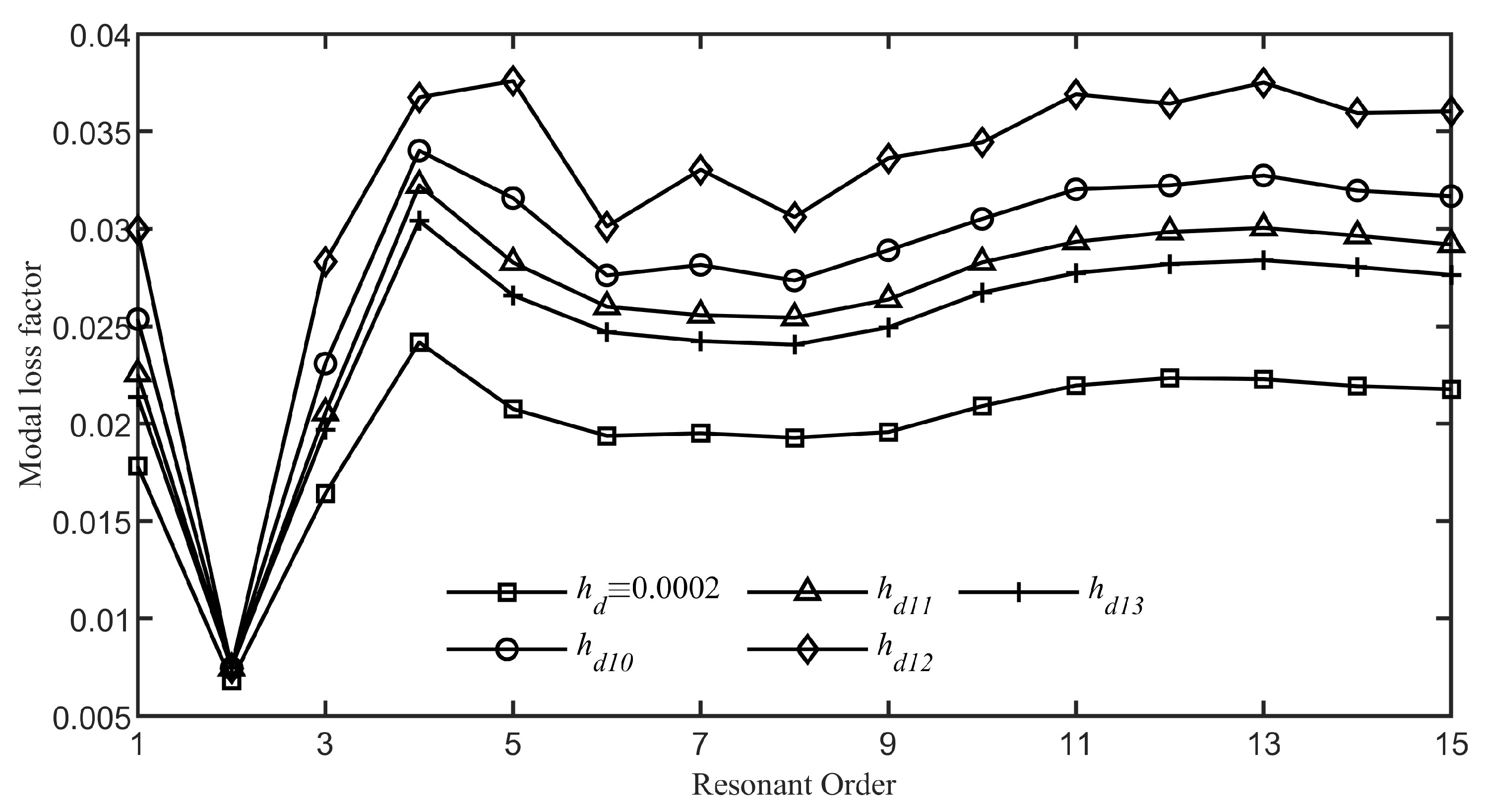
The graphical representations of the functions from Equation (34) closely resemble those shown in Figure 8; therefore, no further graphics are provided here. Figure 17 demonstrates the intensified ABH effect achieved by employing diverse thickness variation functions, as defined in Equation (34). The results obtained by customizing the damping layer’s thickness with functions $h_{d10}$ to $h_{d13}$ are superior to those of a uniform thickness. Notably, Figure 17 reveals that the function $h_{d12}$ yields the most significant ABH effect among the thickness variation functions. This indicates that focusing a higher concentration of damping material at the ABH tip and diminishing it as we move away from the tip significantly boosts the performance compared to an even distribution.

5.3. Optimization of the Damping Layer’s Position and Thickness

Employing the optimization technique for the damping layer thickness function, as detailed in the preceding section, Figure 18 depicts the fitting accuracy of the BP network post-training with Matlab software. The BP neural network has determined the following optimal thickness variation function for the damping layer:

$$h_{dp}\left(x\right)={\displaystyle \frac{9}{16}}{\left(\right|x-0.22|-0.04)}^2,x\in [0.18,0.26].$$

(35)

Figure 18 displays the graphical depictions of the functions $h_{dp}$ and $h_{d12}$, which are specified by Equations (34) and (35), respectively. Figure 19 presents a comparison of the impact on the ABH effect exerted by damping layer thicknesses varied according to the functions $h_{dp}$ and $h_{d12}$. It is evident that with the increase in resonance order, the modal loss factors for the system with the damping layer thickness following the function $h_{d12}$ tend to stabilize at approximately 0.036, while for the system with the damping layer thickness following the function $h_{dp}$, these factors stabilize at around 0.038. The mean modal loss factor for the first fifteen modes of the system with the damping layer thickness set by the function $h_{d12}$ is 0.0323, whereas for the function $h_{dp}$, it is 0.0338, which is roughly $4.6\%$ higher compared to the scenario with $h_{d12}$.

Comparing Figure 20 with Figure 13, it can be observed that when the same mass of damping layer material is applied (after optimizing the thickness of the damping layer using the BP algorithm), the average value of the first fifteen modal loss factors of the modified ABH beam structure (as shown in Figure 15) increases by approximately $15\%$ compared to before the modification (as shown in Figure 1). This indicates that when the truncation thickness $h_0$ of the ABH beam shown in Figure 15 cannot be reduced, the ABH effect can be enhanced by adding a segment with constant thickness $h_0$ within $[x_{y1},x_{y2}]$. To achieve better effects, the length of the segment $[x_{y1},x_{y2}]$ can be further optimized using the BP algorithm.

6. Conclusions

This paper investigates the impact of changing the geometric characteristics of damping layers on the energy dissipation capabilities of a symmetric ABH beam. The utilization of the BP algorithm is proposed to optimize the shape variation of the damping layer. Initially, a semi-analytical solution for the ABH beam’s vibration behavior is derived using the GEM, and the accuracy of this solution is confirmed by comparing it against results from the FEM. Next, leveraging the semi-analytical solution, an analysis of the impact of damping layer parameters, including position, thickness, and shape, on the ABH effect is conducted. Under the premise of maintaining a constant mass of the damping layer, a thickness variation function with a good energy dissipation effect is preliminarily selected. Subsequently, a BP neural network is trained based on the database generated by the semi-analytical solution to optimize the thickness variation function. This study reveals that the damping layer’s geometry has a more intricate impact on performance than previously understood. The BP algorithm stands out as a powerful tool for enhancing the performance evaluation of ABH structures amidst a variety of factors. The optimization analysis conducted using the BP neural network suggests that achieving an effective ABH effect does not require the application of a damping layer across the entire ABH section. The optimal configuration involves maximizing the damping layer thickness at the ABH tip, followed by a rapid decrease in thickness as one moves away from the tip. It is deemed unnecessary to apply a damping layer in areas that are far from the tip.

By appropriately stretching the ABH beam along the truncation thickness while keeping the thickness constant, this paper also optimizes the thickness of the damping layer for the modified ABH beam structure. This study finds that with the same mass of damping layer attached, the modified ABH beam structure can exhibit better energy dissipation effects. This is a novel approach that further enhances the energy dissipation performance of ABH beams without reducing the truncation thickness. Based on the research approach of this paper, the length of the stretched section in the ABH beam can be further optimized using the BP algorithm to achieve better energy dissipation effects. The research in this paper helps to gain a deeper understanding of the impact of the damping layer on the energy dissipation effect of ABH beams.