Study on Vibration Characteristics of Multi-Beam Structures with Stick and Slip at Joints

Abstract

Stick–slip phenomena may manifest at the joints during cyclic vibrations in beam structures connected by some forms of joint. This work incorporates the sticking–slip effect of joint connections into the dynamic analysis framework of multi-beam structures through changes in friction forces. The system characteristic equation is solved using the incremental harmonic balance method, the vibration characteristics of the connected structure are explored through the dynamic response, and the accuracy of the model established in this paper is verified through experiments. The equivalent stiffness and damping changes of a connecting beam under different connection states are investigated for the first time. The research indicates that the “tracking” phenomenon, induced by abrupt damping and resonance frequency variations due to low contact pressure and a low friction coefficient, leads to a relatively stable vibration response amplitude across an extended frequency range. This results in the gradual attenuation of resonance peaks within the frequency response curve, giving rise to a defined resonance frequency range. As connection stiffness diminishes, the system demonstrates characteristics of internal resonance. In addition, the influence characteristics of external excitation and connection joint position on the vibration response of multi-beam structures are also explored. This model provides an effective method for studying the vibration problems of complex beam frame structures.

1. Introduction

Beam structures are fundamental components in modern machinery, and the dynamic analysis of such structures has always been a significant research focus for scholars [1]. Theoretical models, including those of Euler–Bernoulli [2], Timoshenko [3], Rayleigh [4], and the shear deformation beam [5], have been proposed and extensively investigated. Various numerical methods such as the semi-analytical method [6], Galerkin method [7], Rayleigh–Ritz method [8], dynamic stiffness method [9], differential quadrature method [10], and finite element method [11] have demonstrated remarkable capabilities in accurately predicting the dynamic behavior of beam structures.

Engineering systems commonly involve beam structures that have diverse types of connections. To accurately describe their mechanical properties, various mechanical models have been developed based on different connection conditions [12]. For instance, theoretical models employing stiffness damping [13], the Iwan model utilizing the density function integral method [14,15,16], the Valanis model [17], the Bouc–Wen model [18,19], and diverse finite element models [20,21] have been constructed. Analyzing structural vibrations essentially involves solving boundary value problems consisting of governing differential equations and their corresponding boundary conditions. This collective set of connections and conditions can be referred to as the boundary value problem. A research approach that incorporates spring stiffness to simulate boundaries and connections [22,23,24,25,26,27,28] enables a more comprehensive analysis of vibration characteristics within the framework of linear theory. Wu et al. [29] used an improved Fourier series and Rayleigh–Ritz method to establish an analysis model for the self-vibration characteristics of continuous multi-span beams with concentrated mass. Hao et al. [30] used an improved Fourier–Ritz method to study the free vibration problem of the double-beam system under general boundary conditions. Li et al. [31] provided a general method for analyzing the dynamic characteristics of multi-span beam systems under arbitrary boundary conditions, where the coupling between adjacent beams is described by linear and rotational springs, and each beam is independently elastically constrained/coupled. Based on the Fourier series, the displacement basis function is established, and continuity is not required at the connection, which has strong scalability and can be used for modal analysis research into periodic beam structures. Numerical examples show that under general boundary and coupling conditions, the modal characteristics of the multi-beam system can be accurately calculated.

In the linear theoretical framework, the idealized description of the linear stiffness in the connection transitions from ‘free’ to ‘clamped’. However, when considering beam structures connected by bolts or rivets, it is important to account for the relative displacement of the assembly joint surface, caused by transverse vibration, which can lead to nonlinear behavior due to frictional viscous effects [32]. The study conducted by Li et al. [33] utilized nonlinear stiffness and damping to characterize the axial connection of the rotor system and established a dynamic model of a rotor-bearing system incorporating bolted joints. The impact of connection looseness faults and other factors on the system’s dynamic and mechanical behavior was investigated by analyzing the vibration waveform and frequency spectra. The analysis of nonlinear behavior [34], which incorporates the influence of friction on damping [35], is essential for accurately predicting the dynamic characteristics of structures and facilitating structural design.

Joglekar [36] investigated the nonlinear mixing of Timoshenko beams with breathing cracks by considering the crack interface as a bilinear stiffness-connected structure and incorporating two springs to simulate the local bending and shear deformations induced by the crack. The intermittent contact between the two crack surfaces was simulated by switching between intact and cracked beams. The wavelet finite element method was employed to explain the iterative process of solving the nonlinear equation system required for interpreting the solution while analyzing the phenomenon of nonlinear mixing in a beam with lateral edge cracks. Zhao et al. [37] proposed a dynamic analysis model for a generally constrained double-beam structure with nonlinear stiffness and damping in its connections, and the Galerkin truncated method (GTM) was employed to solve the nonlinear governing equations of the double-beam structure. The study conducted by Krack et al. [38] investigated the modal coupling resulting from joint friction and explored passive vibration reduction techniques involving friction. Under proximity to the conjugate eigenfrequency, the nonlinear characteristics of friction give rise to nonlinear modal interaction. When harmonic excitation is applied in the vicinity of a specific mode’s natural frequency, significant contributions to the vibration response can be attributed to exciting another mode through nonlinear energy transfer. Within the resonance range, adjusting the ratio between the first two natural frequencies allows the triggering or suppression of mode interactions. In certain scenarios, vibration levels can decrease due to energy redistribution.

Tufekci et al. [39] introduced dry friction at the contact interface of an imperfectly supported cantilever and proposed an analytical solution for predicting the nonlinear dynamic behavior of a friction-clamped rod under axial and torsional motion. The dynamic behavior of a cantilever beam supported by contact forces with friction was analyzed by solving the control differential equation using a numerical method known as frequency-time harmonic balance, and the influence of contact parameters on the system’s behavior was investigated. Tang et al. [40] investigated the soft nonlinearity of the structural response curve of a bolted connection between cylinders by incorporating a viscous friction model into the joint and calculating the resulting connection force.

Loose connections [41,42] are a prevalent type of mechanical structural fault. The literature mentioned above shows that the characteristic representation of structural fault diagnosis can be enhanced by investigating the laws of the influence of nonlinear mechanical state changes on structural vibration characteristics. Specifically, an in-depth understanding of the nonlinear modalities of connection structures [43] and their responses is crucial for implementing damping measures using friction-damping nonlinear characteristics [44,45]. This can be developed into strategies for designing vibration suppression friction contacts that minimize energy transmission or maximize energy dissipation [46,47].

In summary, the existing research has primarily focused on developing friction force function expressions and a dynamic analysis framework that incorporates friction force into structural analysis, ranging from discrete system analysis for nonlinear connection conditions with friction function expressions [48,49,50,51] to continuous structure analysis considering the dynamics of friction force [52,53,54]. This work will mainly examine the beam structure that often appears in actual projects, and will analyze the influence of changes in connection parameters on the structural connection state and vibration response, which lays the foundation for vibration reduction and complex structure design.

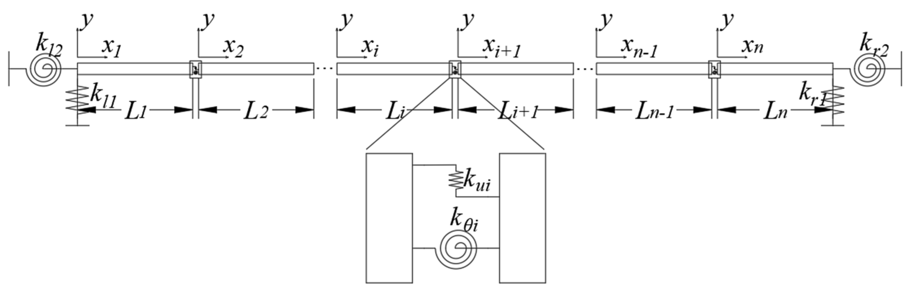
2. Theoretical Modeling

The structural model is shown in Figure 1. The lengths of the beams are L₁, L₂, …, L_n, with the right end of each beam serving as the origin to establish the coordinate system. This section will derive the vibration control equation for a double-beam connection structure and then expand the equation to a multi-beam connection situation by increasing the matrix dimensions.

2.1. Energy Equation of Beam Structure

The expressions of the kinetic energy T_i and the strain potential energy V_i of each beam are as follows:

$$T_i={\displaystyle \frac{1}{2}}{{\displaystyle {\int }_0^{L_i}{\rho }_i{S}_i\left(\frac{\partial u_i}{\partial t}\right)}}^{2}d{x}_i$$

(1)

$$V_i={\displaystyle \frac{1}{2}}{{\displaystyle {\int }_0^{L_i}EI\left(\frac{{\partial }^2{u}_i}{\partial x_i^2}\right)}}^{2}d{x}_i$$

(2)

where ρ_i represents the mass density of the beam, S_i denotes its cross-sectional area, u_i signifies the vibration displacement, E represents the Young’s modulus of the material, and I is the moment of inertia of the section; i = 1 or 2 represents the kinetic energy of beam 1 or 2, and the same is true for i below. The spring stiffness is introduced to simulate the boundary conditions at the boundary end of the beam, where k_l1 and k_r1 are the boundary translational stiffness, while k_l2 and k_r2 are the rotational stiffness, as shown in Figure 1. Therefore, the energy descriptions of the boundary constraints V_l1, V_l2, V_r1, V_r2 are, respectively, as follows:

$$\left\{\begin{array}{l}{V}_{l1}={\displaystyle \frac{1}{2}}{k}_{l1}{\left(u_1{|}_{x_1=0}\right)}^2\\ V_{l2}={\displaystyle \frac{1}{2}}{k}_{l2}{\left({\displaystyle \frac{\partial u_1}{\partial x_1}}{|}_{x_1=0}\right)}^2\\ V_{r1}={\displaystyle \frac{1}{2}}{k}_{r1}{\left(u_n{|}_{x_n=L_n}\right)}^2\\ V_{r2}={\displaystyle \frac{1}{2}}{k}_{r2}{\left({\displaystyle \frac{\partial u_n}{\partial x_n}}{|}_{x_n=L_n}\right)}^2\end{array}\right..$$

(3)

Disregarding the interconnections, the total kinetic energy and potential energy can be expressed as T = T₁ + T₂ + … + T_n and V = V₁ + V₁ + … + V_n + V_l1 + V_l2 + V_r1 + V_r2. The Dirac delta function δ is used to express the external excitation force as a distributed force, and its mathematical expression is as follows:

$$f(x_i,t)=\delta (x_i-x_0)F_0{e}^{(j{\omega }_{0}t)}.$$

(4)

The excitation amplitude is denoted as F₀, the coordinates of the operating point are designated as x₀, and the excitation frequency is represented by ω₀. The expression of the work term W_ext can be obtained as follows:

$$W_{ext}={\displaystyle {\int }_0^{L_i}f(x_i,t)u_i(x_i,t)dx}=F_0{e}^{j{\omega }_{0}t}{\mathsf{\Phi }}_i(x_0)T_i(t).$$

(5)

Considering the friction at the connection during transverse vibrations, the equivalent stiffness K_eq and damping C_eq are utilized to characterize the relationship between the interface connection force, damping, and stiffness at the connection:

$$\left\{\begin{array}{l}{f}_{u1}=K_{eq}(u_1-u_2)+C_{eq}({\dot{u}}_1-{\dot{u}}_2)\\ f_{u2}=K_{eq}(u_2-u_1)+C_{eq}({\dot{u}}_2-{\dot{u}}_1)\end{array}\right..$$

(6)

Therefore, the virtual work done by the translational connecting force at the connection is as follows:

$$\left\{\begin{array}{l}\delta W_{f_{u1}}=\left[K_{eq}(u_1-u_2)+C_{eq}({\dot{u}}_1-{\dot{u}}_2)\right]\delta u_1\\ \delta W_{f_{u2}}=\left[K_{eq}(u_2-u_1)+C_{eq}({\dot{u}}_2-{\dot{u}}_1)\right]\delta u_2\end{array}\right..$$

(7)

The connecting force resulting from relative rotation is as follows:

$$\left\{\begin{array}{c}{M}_1=k_{\theta }\left({\displaystyle \frac{\partial u_1}{\partial x_1}}-{\displaystyle \frac{\partial u_2}{\partial x_2}}\right)\\ M_2=k_{\theta }\left({\displaystyle \frac{\partial u_2}{\partial x_2}}-{\displaystyle \frac{\partial u_1}{\partial x_1}}\right)\end{array}\right..$$

(8)

The virtual work of the rotating connecting force can be written as the following:

$$\left\{\begin{array}{c}\delta W_{M_1}=k_{\theta }\left({\displaystyle \frac{\partial u_1}{\partial x_1}}-{\displaystyle \frac{\partial u_2}{\partial x_2}}\right)\delta {\displaystyle \frac{\partial u_1}{\partial x_1}}\\ \delta W_{M_2}=k_{\theta }\left({\displaystyle \frac{\partial u_2}{\partial x_2}}-{\displaystyle \frac{\partial u_1}{\partial x_1}}\right)\delta {\displaystyle \frac{\partial u_2}{\partial x_2}}\end{array}\right..$$

(9)

Thus, the total virtual work of the connecting force can be obtained as follows:

$$\delta W=\delta W_{f_{u1}}+\delta W_{f_{u2}}+\delta W_{M_1}+\delta W_{M_2}.$$

(10)

2.2. Improved Fourier Series Expansion Vibration Displacement

After separating the time and space variables, vibration displacement u_i can be written as follows:

$$u_i={\Phi }_i(x_i)\cdot T_i(t).$$

(11)

This includes the basis function Φ_i(x_i) and the time term T_i(t). After employing the improved Fourier series to expand the basis function Φ_i(x_i), the form is as follows:

$${\Phi }_i(x_i)={\displaystyle \sum _{k=0}^{\infty }{a}_{k}cosk\pi \frac{x_i}{L_i}}+a_{i1}^f{\xi }_{i1}\left(x_i\right)+a_{i2}^f{\xi }_2\left(x_i\right)+a_{i3}^f{\xi }_{i3}\left(x_i\right)+a_{i4}^f{\xi }_{i4}\left(x_i\right)$$

(12)

where ξ_i1(x), ξ_i2(x), ξ_i3(x), ξ_i4(x) are boundary smooth terms used to eliminate the discontinuity of multi-order derivatives of displacement function at the boundary in the following form:

$$\left\{\begin{array}{c}{\xi }_{i1}\left(x_i\right)={\displaystyle \frac{9L_i}{4\pi }}\sin \left({\displaystyle \frac{\pi x_i}{2L_i}}\right)-{\displaystyle \frac{L_i}{12\pi }}\sin \left({\displaystyle \frac{3\pi x_i}{2L_i}}\right)\\ {\xi }_{i2}\left(x_i\right)=-{\displaystyle \frac{9L_i}{4\pi }}\cos \left({\displaystyle \frac{\pi x_i}{2L_i}}\right)-{\displaystyle \frac{L_i}{12\pi }}\cos \left({\displaystyle \frac{3\pi x_i}{2L_i}}\right)\\ {\xi }_{i3}\left(x_i\right)={\displaystyle \frac{L_i^3}{{\pi }^3}}\sin \left({\displaystyle \frac{\pi x_i}{2L_i}}\right)-{\displaystyle \frac{L_i^3}{3{\pi }^3}}\sin \left({\displaystyle \frac{3\pi x_i}{2L_i}}\right)\\ {\xi }_{i4}\left(x_i\right)=-{\displaystyle \frac{L_i^3}{{\pi }^3}}\cos \left({\displaystyle \frac{\pi x_i}{2L_i}}\right)-{\displaystyle \frac{L_i^3}{3{\pi }^3}}\cos \left({\displaystyle \frac{3\pi x_i}{2L_i}}\right)\end{array}\right..$$

(13)

Therefore, transverse vibration displacement can be written in the following matrix form:

$$u_i=U_i^T{\alpha }_i{T}_i(t).$$

(14)

where $U_i^T$ is the basis function vector, which is only related to the displacement variable, and α_i is the response coefficient vector:

$$\left\{\begin{array}{c}{U}_i^T=[1,cos\pi {\displaystyle \frac{x_i}{L_i}},\cdots ,\cos n\pi {\displaystyle \frac{x_i}{L_i}},{\xi }_{i1}\left(x_i\right),{\xi }_{i2}\left(x_i\right),{\xi }_{i3}\left(x_i\right),{\xi }_{i4}\left(x_i\right)]\hfill \\ {\alpha }_i=[a_{i0},\cdots ,a_{in},a_{i1}^f,a_{i2}^f,a_{i3}^f,a_{i4}^f{]}^T\hfill \end{array}\right..$$

(15)

After utilizing the first-order harmonic expansion to extend the time term [40], the vibration displacement can be written as follows:

$$u_i=U_i^T{\alpha }_i\left(a_i^c\cos (\omega t)+a_i^s\sin (\omega t)\right)=U_i^T{\alpha }_i{p}_i.$$

(16)

where a_i^c and a_i^s are the response coefficient vectors corresponding to the first-order cosine and sine wave, respectively, and p_i is the generalized time vector.

2.3. Nonlinear Connecting

In the case of friction, the connecting force between adjacent beams resulting from relative displacement is represented as f_u. It becomes essential to account for the energy variations in the system caused by the motion state of the joint. In the vibration process, the connection interface will experience changes in stick and slip. A piece-wise function represents the connection force:

$$f_u=\left\{\begin{array}{c}{k}_u\left[u_1-u_2-(u_{1e}-u_{2e})\right]+f_{ue}\\ {\mu }_f{F}_N\\ -{\mu }_f{F}_N\end{array}\right.\begin{array}{c}\begin{array}{cc}& u_d=0\end{array}\\ \begin{array}{cc}& u_d>0\end{array}\\ \begin{array}{cc}& u_d<0\end{array}\end{array}\begin{array}{c}\\ \\ \end{array}\begin{array}{c}\mathrm{stick}\\ \mathrm{positive} \mathrm{slip}\\ \mathrm{negative} \mathrm{slip}\end{array}.$$

(17)

where k_u is the transitional connection stiffness; u_1e, u_2e, and f_ue are the initial values of u₁, u₂, and f_u at the beginning of the stick state; and u_d = u_1r − u_2l is the relative displacement of the two beams at the connection. When it is zero, the interface is in the stick state, and once relative displacement occurs, the interface enters a state of either positive or negative sliding. F_N is the contact pressure and μ_f is the friction coefficient of the contact interface.

Taking the joint of beam 1 and beam 2 as an example, the vibration displacement at both ends of the structural connection interface is as follows:

$$\begin{array}{c}{u}_{1r}=u_1{|}_{x_1=L_1}=U_{11}^T\left(a_1^c\cos (\omega t)+a_1^s\sin (\omega t)\right)=U_{11}^T{p}_1\hfill \\ u_{2l}=u_2{|}_{x_2=0}=U_{20}^T\left(a_2^c\cos (\omega t)+a_2^s\sin (\omega t)\right)=U_{20}^T{p}_2\hfill \end{array}.$$

(18)

Thus, the relative displacement u_d at the joint can be expressed as follows:

$$u_d=u_{1r}-u_{2l}=\chi \cos (\vartheta )$$

(19)

where

$$\vartheta =\omega t+\phi ,\chi =\sqrt{{(A_1-B_1)}^2+{(A_2-B_2)}^2}$$

and

$$A_1=U_{11}^T{a}_1^c,A_2=U_{11}^T{a}_1^s,B_1=U_{20}^T{a}_2^c,B_2=U_{20}^T{a}_2^s,\cos (\phi )={\displaystyle \frac{(A_1-B_1)}{\chi }},\sin (\phi )={\displaystyle \frac{(A_2-B_2)}{\chi }}.$$

The corresponding velocity and acceleration are as follows:

$$\left\{\begin{array}{l}{\dot{u}}_d=-\omega \chi \sin (\vartheta )\\ {\ddot{u}}_d=-{\omega }^2\chi \cos (\vartheta )\end{array}\right.$$

(20)

Generalized time terms can denote the spatial relationships on both sides of the connection. Accordingly, the connection state (Equation (12)) can be transformed into a description in the time domain. By deconstructing the mechanical state variations at the joint interface throughout a vibration cycle, the vibration process can be divided into four dynamic transition processes: from stick to positive slip state, from positive slip to stick state, from stick to negative slip state, and from negative slip to stick state. When defining four of these generalized time nodes ϑ, the values are $\vartheta ={\vartheta }_P^S$, which means that the stick changes to the positive slip state and the transitional connection is f = μ_fF_N, i.e., $f_u({\vartheta }_P^S)=k_u\left[u_1({\vartheta }_P^S)-u_2({\vartheta }_P^S)-(u_{1e}-u_{2e})\right]+f_{ue}={\mu }_{f}N$, $\vartheta ={\vartheta }_S^P$ means that from positive slip to stick, the connection force is f = μ_fF_N, in which case, ${\dot{u}}_d=0$, ${\ddot{u}}_d<0$; $\vartheta ={\vartheta }_N^S$ means that from stick to negative slip, the connection force is f = −μ_fF_N; $\vartheta ={\vartheta }_S^N$ means that from negative slip to stick, the connection force is f = −μ_fF_N; where ${\dot{u}}_d=0$, ${\ddot{u}}_d>0$. That is, the change in mechanical state occurring at the joint can be expressed as follows:

$$\left\{\begin{array}{l}{f}_u({\vartheta }_P^S)=k_u\left[u_1({\vartheta }_P^S)-u_2({\vartheta }_P^S)-(u_{1e}-u_{2e})\right]+f_{ue}={\mu }_f{F}_N\\ \omega \chi \sin ({\vartheta }_S^P)=0, -{\omega }^2\chi \cos ({\vartheta }_S^P)<0\\ f_u({\vartheta }_N^S)=k_u\left[u_1({\vartheta }_N^S)-u_2({\vartheta }_N^S)-(u_{1e}-u_{2e})\right]+f_{ue}=-{\mu }_f{F}_N\\ \omega \chi \sin ({\vartheta }_S^N)=0, -{\omega }^2\chi \cos ({\vartheta }_S^N)>0\end{array}\right.$$

(21)

Therefore, we can conclude the following:

$$\left\{\begin{array}{l}{\vartheta }_S^P=0\\ {\vartheta }_S^N=\pi \\ {\vartheta }_P^S=\pi +{\cos }^{-1}\left(1-{\displaystyle \frac{2{\mu }_f{F}_N}{\chi k_u}}\right)\\ {\vartheta }_N^S={\cos }^{-1}\left(1-{\displaystyle \frac{2{\mu }_f{F}_N}{\chi k_u}}\right)\end{array}\right.$$

(22)

The segmented representation of the bonding force is as follows:

$$f_u=\left\{\begin{array}{c}{k}_u(\cos (\vartheta )-1)+{\mu }_f{F}_N\\ -{\mu }_{f}N\\ k_u(\cos (\vartheta )-1)-{\mu }_f{F}_N\\ {\mu }_{f}N\end{array}\right.\begin{array}{c}\begin{array}{cc}& {\vartheta }_S^P\le \vartheta \le {\vartheta }_N^S\end{array}\\ \begin{array}{cc}& {\vartheta }_N^S\le \vartheta \le {\vartheta }_S^N\end{array}\\ \begin{array}{cc}& {\vartheta }_S^N\le \vartheta \le {\vartheta }_P^S\end{array}\\ \begin{array}{cc}& {\vartheta }_P^S\le \vartheta \le 2\pi \end{array}\end{array}$$

(23)

The translational connecting force periodic function can be expanded by a first-order Fourier series, as follows:

$$f_u={\displaystyle \frac{f_0}{2}}+f_c\cos \vartheta +f_s\sin \vartheta$$

(24)

where the standard integral form of the Fourier coefficient is the following:

$$\left\{\begin{array}{l}{f}_0=0\\ f_c={\displaystyle \frac{1}{\pi }}{\displaystyle {\int }_0^{2\pi }{f}_u\cos (\vartheta )d\vartheta }={\displaystyle \frac{\chi k_u}{\pi }}\left[{\vartheta }_N^S-\cos ({\vartheta }_N^S)\sin ({\vartheta }_N^S)\right]\\ f_s={\displaystyle \frac{1}{\pi }}{\displaystyle {\int }_0^{2\pi }{f}_u\sin (\vartheta )d\vartheta }={\displaystyle \frac{\chi k_u}{\pi }}\left[{\cos }^2({\vartheta }_N^S)-1\right]\end{array}\right.$$

(25)

Following Equations (6), (24), and (25), the equivalent stiffness K_eq and damping C_eq can be represented as follows [55]:

$$\left\{\begin{array}{c}{K}_{eq}={\displaystyle \frac{f_c}{\chi }}={\displaystyle \frac{k_u}{\pi }}\left[{\vartheta }_N^S-\cos \left({\vartheta }_N^S\right)\sin \left({\vartheta }_N^S\right)\right]\hfill \\ C_{eq}={\displaystyle \frac{f_s}{-\omega \chi }}={\displaystyle \frac{k_u}{\omega \pi }}\left[1-{\cos }^2\left({\vartheta }_N^S\right)\right]\hfill \end{array}\right.$$

(26)

2.4. Theoretical Solution of Displacement Series Coefficients

The kinetic energy T, potential energy V, work term of external force, and virtual work of the connecting force for the system have been given in Equations (1)–(10). The Lagrange equation of the vibration system can be obtained as follows:

$${\displaystyle \frac{d}{dt}}{\displaystyle \frac{\partial T}{\partial \dot{X}}}-{\displaystyle \frac{\partial T}{\partial X}}+{\displaystyle \frac{\partial V}{\partial X}}+{\displaystyle \frac{\partial (\delta W)}{\partial (\delta X)}}={\displaystyle \frac{\partial W_{ext}}{\partial X}}$$

(27)

where X is the generalized time vector of the system:

$$X=\left[\begin{array}{l}{p}_1\\ p_2\end{array}\right].$$

(28)

The vibration control equation of the system in the case of nonlinear connection can be expressed as follows:

$$M\ddot{X}+KX+f_b(X,\dot{X})=F_{\omega }(t).$$

(29)

Here, M is the mass matrix, K is the stiffness matrix, and $f_b(X,\dot{X})$ is the nonlinear continuous force matrix, which is related to the nonlinear continuous force work derived in Section 2.3. The specific expressions of each matrix are given in Appendix A. Equation (29) can be solved by the harmonic incremental balance method.

3. Result Analysis and Discussion

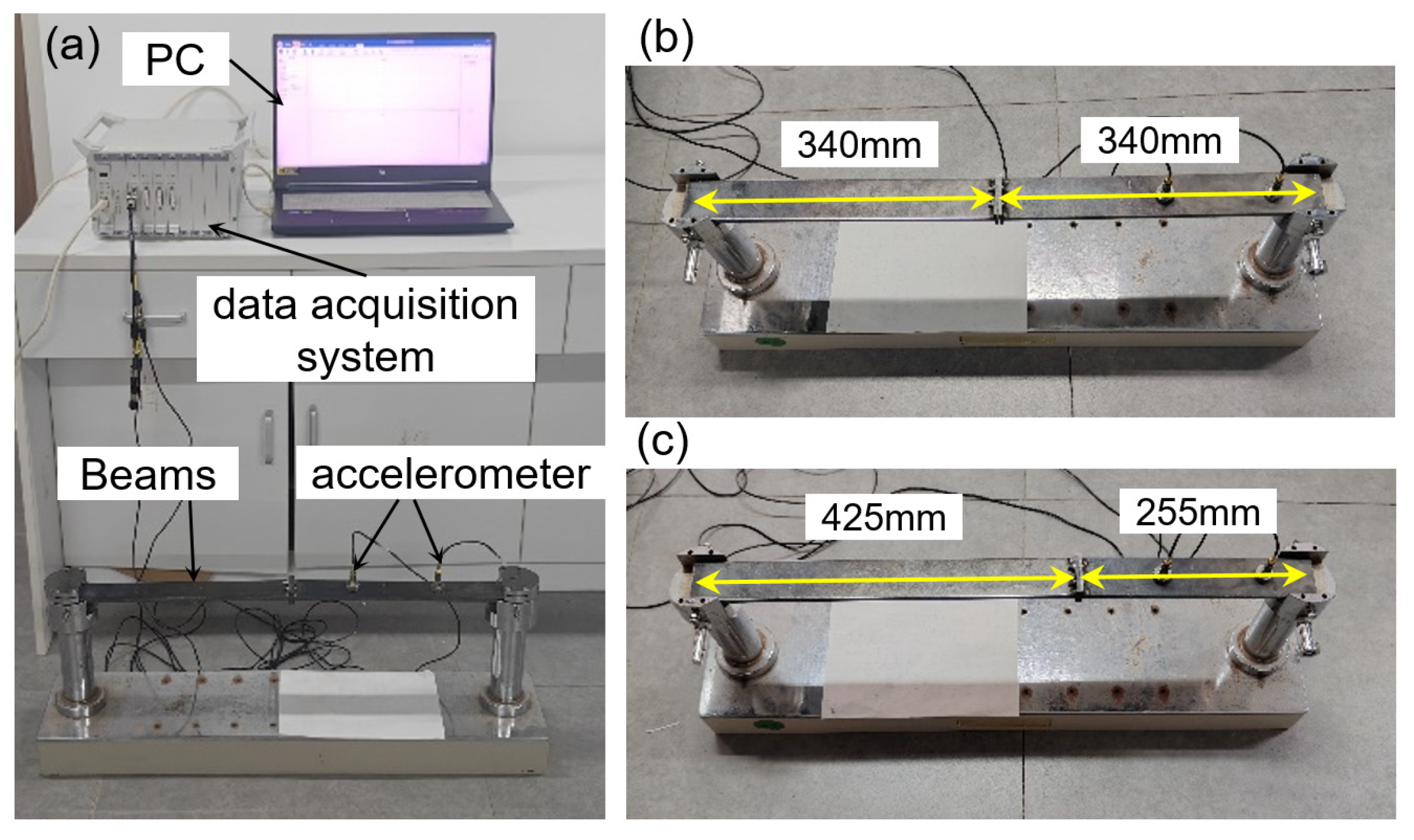
In this section, to investigate the effects of various parameters on the nonlinear response and connection state of the structure, the vibration responses and connection state changes of the structure under different parameters are analyzed based on the established model. The incremental harmonic balance method is used to solve the structural vibration control equation. The Newton iteration method is used in the solving process, and the response coefficient vector in the case of a linear response is the initial iteration value of a_i^c.

3.1. Validation

In this section, the accuracy of the model is initially verified through experiments. For a unified quantitative comparison, the connection conditions of the beam structure are designed as bolted fastening connections, while the model presented in this paper can also easily realize the degradation of connection conditions through external force virtual work terms. The experimental system is shown in Figure 2, where DH 1A102E acceleration sensors (resolution factor: 0.002 g, measurement range: ±500 g, frequency response (±10%): 1~10,000 Hz, weight: 5.5 g, and axial sensitivity (23 ± 5 °C): 1 mV/m·s⁻² (9.8 mV/g)) are used to acquire vibration signals, which are then sampled through a DH5922D data acquisition system (frequency response range: DC~100 kHz, input impedance: 10 MΩ + 10 MΩ) and analyzed using a real-time data measurement and analysis software system (Dong-Hua Test DHDAS). The geometric parameters of the two composite beam structures are shown in Figure 2b and Figure 2c, respectively, and the beams have a thickness of H = 8 mm and a width of B = 50 mm. The material density is ρ = 7850 kg/m³ and the elastic modulus is E = 200 GPa. The bolts used are M2 standard threaded, with an equivalent transitional stiffness of 10⁶ N/m and a rotational stiffness of 10³ N·m/rad. Additionally, in the model used in this paper, the theoretical results converge when the truncation number N exceeds 15, which is from multiple verification analyses. As shown in

Table 1. Comparison of natural frequencies of two composite beams.

		Case I			Case II
		Experiment	Present	Error	Experiment	Present	Error
Simply supported	1st	38.156	36.736	3.8%	37.109	35.969	3.1%
	2nd	154.297	155.771	1.0%	146.484	149.145	1.8%
	3rd	322.326	326.375	1.3%	332.031	333.604	0.5%
Clamped	1st	81.055	83.322	2.8%	83.008	85.279	2.7%
	2nd	245.117	241.488	−1.5%	231.445	231.747	0.1%
	3rd	439.453	443.556	0.9%	460.938	458.237	−0.6%

, the comparison of the first three natural frequencies under simply supported and clamped boundary conditions shows that the analysis results of the model in this paper are in good agreement with the experimental results, which can verify the accuracy of the model.

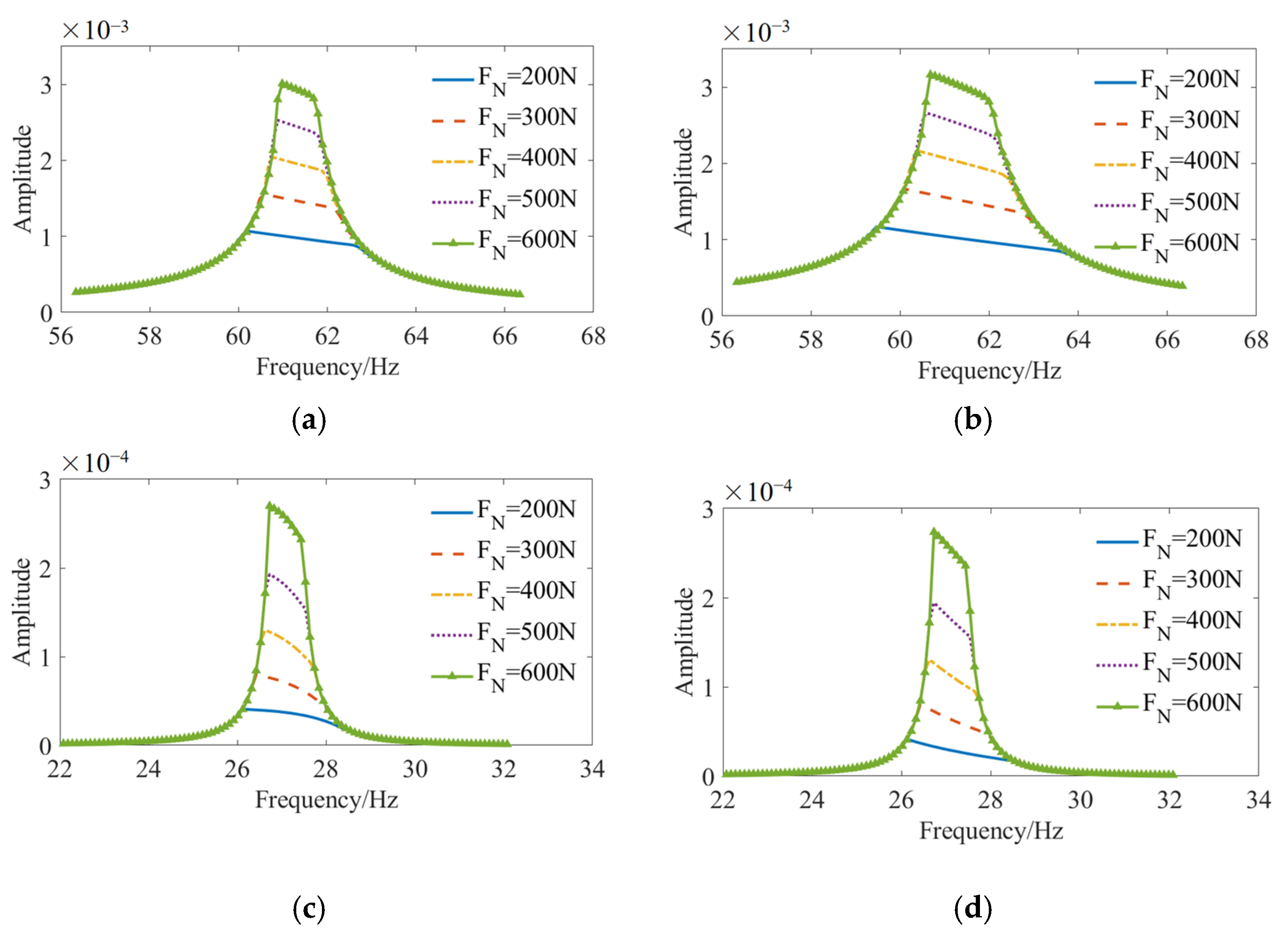
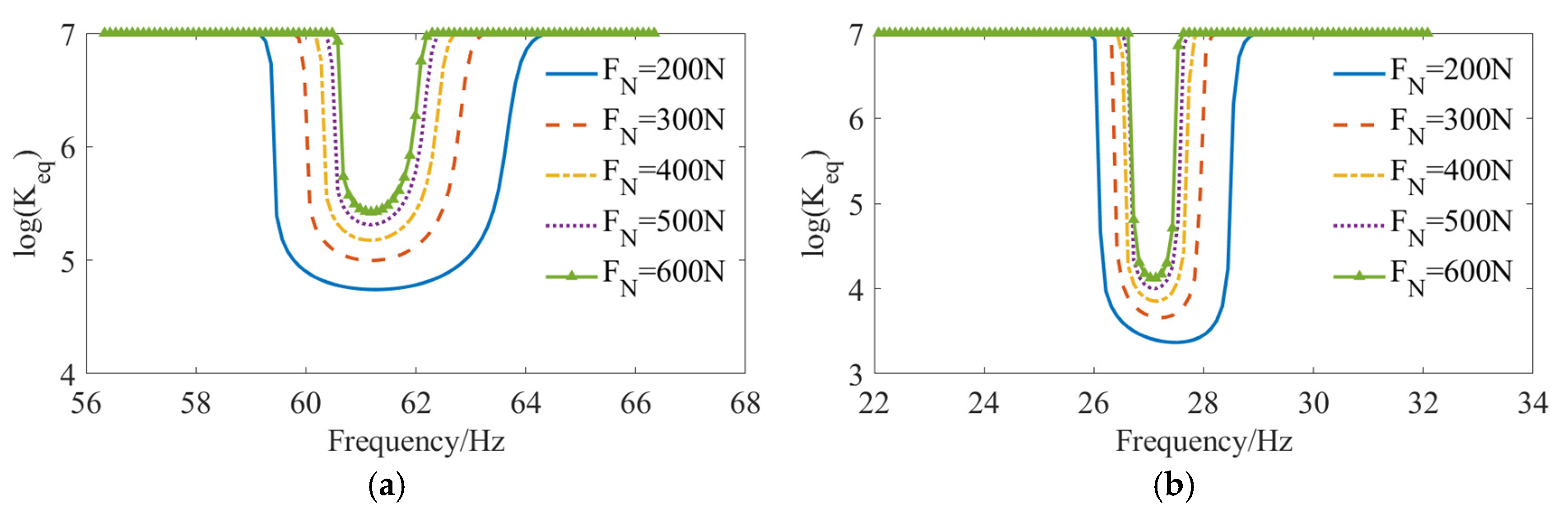
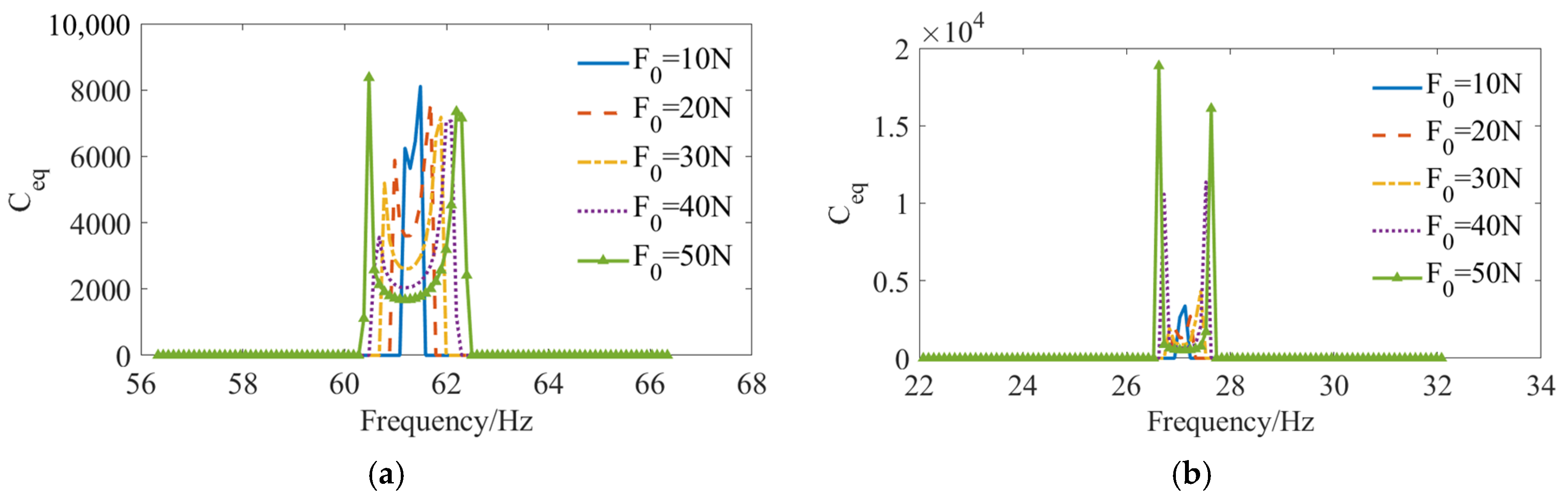
3.2. Response Under Different Contact Pressure Conditions

In the connection force expression, the contact pressure F_N is an important variable whose physical meaning is the preload force in bolt connections and the normal force in other connection situations, which significantly affects the tightness of the connection. In this section, the structural frequency response under different levels of contact pressure will be discussed to analyze the influence of contact pressure on the structural dynamic characteristics. As shown in Figure 3, the frequency response curves of the connection beam structure on both sides of the connection point under different preload conditions are presented, where the connection stiffnesses are k_u = 10⁷ N/m, k_θ = 10⁷ N·m/rad; the friction coefficient is μ = 0.3; the excitation amplitude F₀ of 50 N is applied at the midpoint of beam L₁; and the boundary conditions are fixed support or simply supported. In this section and Section 3.3, Section 3.4 and Section 3.5, the structural dimensions are L₁ = 0.5 m, L₂ = 0.8 m; height is H = 20 mm; and width is B = 20 mm. The excitation frequency range is [ω₁ − 5, ω₁ + 5], where ω₁ represents the first natural frequency under the framework of linear theory. It is evident that with an increase in the preload, the system response curve tends towards the linear frequency response curve, indicating that the structure can be regarded as a linear system under sufficient preload force. As the preload force decreases, the frequency response curve gradually flattens, eliminating the resonance peak and resulting in a range of resonance frequencies. In the low-preload state where the peak is eliminated, the maximum response frequency always remains lower than the linear natural frequency, which is situated at the left end of the resonance interval.

In response to the ‘clipping’ phenomenon of the response peak in the resonance range, Figure 4 and Figure 5 illustrate the variation of equivalent stiffness and damping with excitation frequency under different preload conditions. It is evident that the maximum equivalent stiffness equals the connecting transitional stiffness k_u, which experiences a sharp decrease in the resonance region, where the magnitude of stiffness reduction and the frequency range affected are negatively correlated with the contact pressure. In other words, lower contact pressure leads to a greater reduction in equivalent stiffness and a wider affected frequency range, which clearly corresponds with the frequency response curve.

Within a certain frequency range, due to the reduction in equivalent stiffness, the resonance frequency will shift to the left, resulting in changes to the peak frequency in the frequency response curve corresponding to different pressures. The more the stiffness is reduced, the more the resonance peak frequency will shift to the left and decrease. Through Figure 4, which shows the change in equivalent damping, one can see that the “tracking” phenomenon caused by the sudden shift in damping and the change in resonance frequency results in a relatively stable response amplitude within a larger frequency range for smaller preload forces.

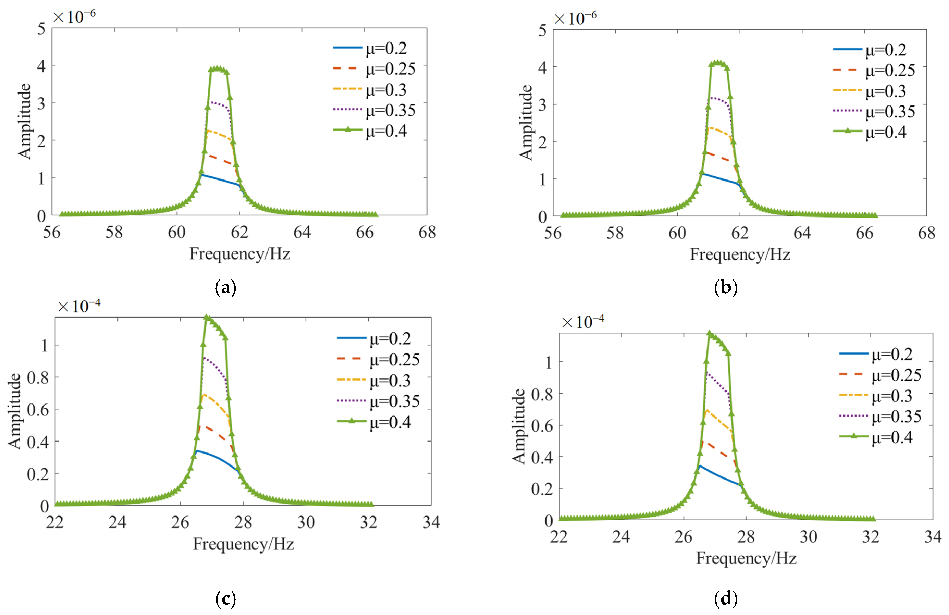
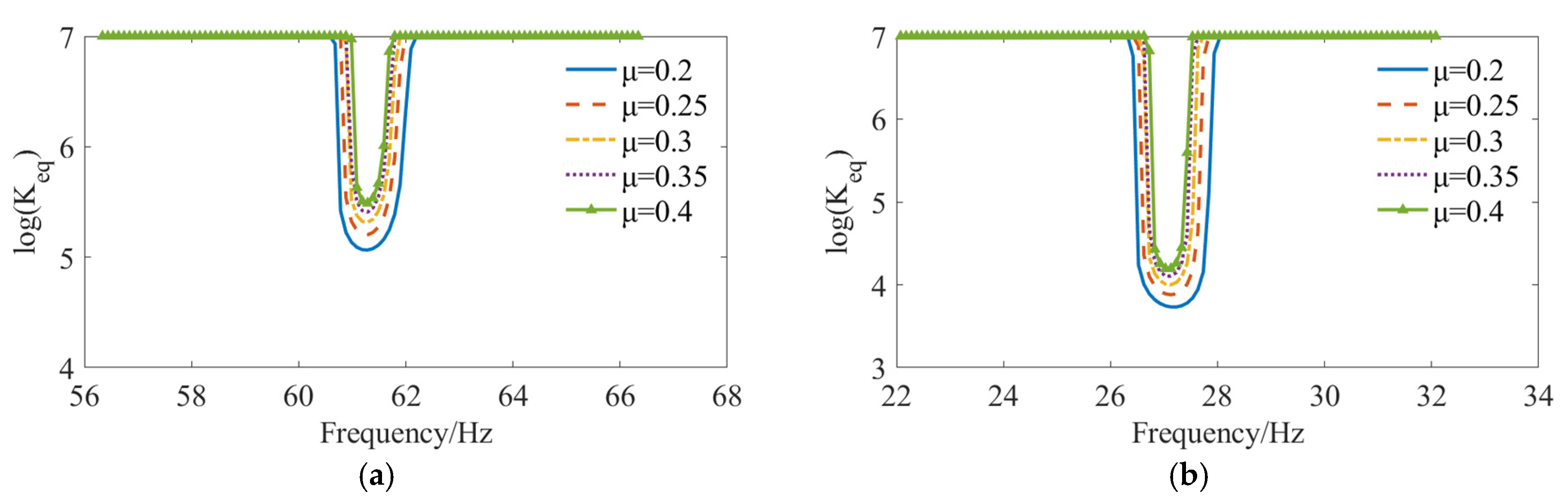
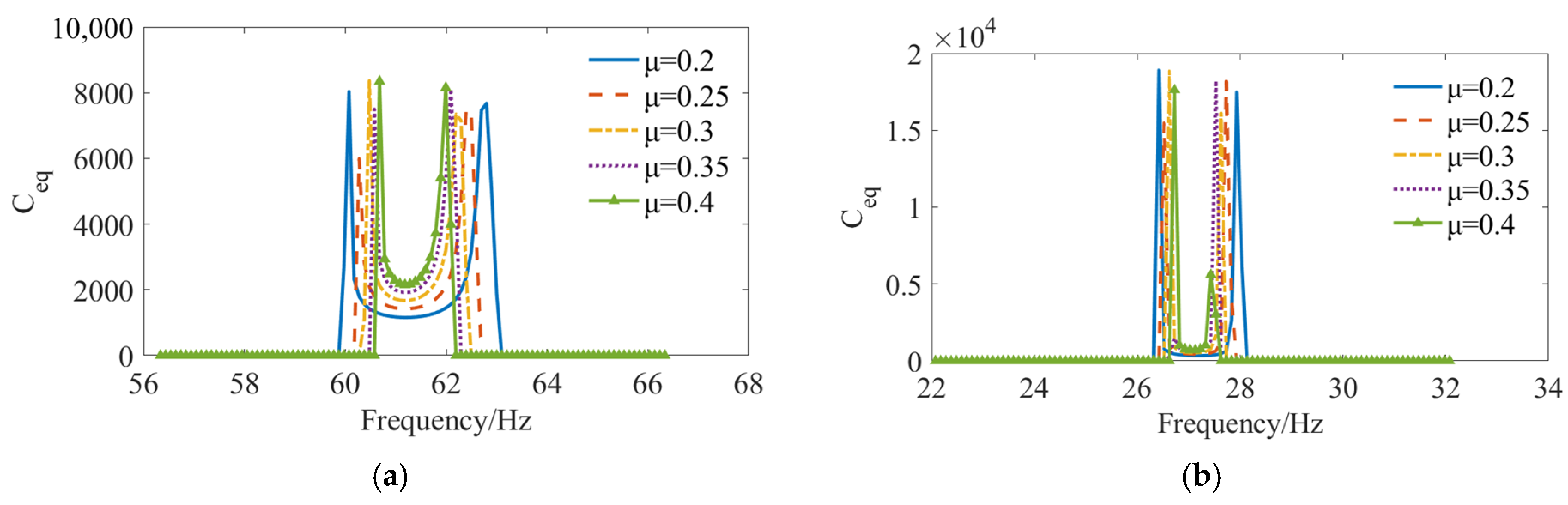
3.3. Structural Amplitude–Frequency Curves with Different Friction Coefficients

In addition to the contact pressure, the friction coefficient is a crucial factor influencing friction force which, in turn, impacts the vibration characteristics of the structure under nonlinear connection conditions. Here, we present the amplitude–frequency curves of the structure under various friction coefficients, as depicted in Figure 6. Figure 7 and Figure 8 illustrate the variation in equivalent connection stiffness and equivalent damping under different friction coefficients, where the external excitation amplitude F₀ = 30 N and the connection preload F_N = 300 N. By comparing Figure 3, Figure 4 and Figure 5, it can be observed that the influence of the friction coefficient on the system characteristics resembles that of the preload. A higher coefficient of friction at the contact interface leads to a frequency response curve for the structure approaching a linear state. With the increase in the friction coefficient, the range of the frequency’s influence on the stiffness becomes narrower. A larger coefficient of friction will impede the initiation of relative sliding between structures, while the sudden shift in stiffness will manifest closer to the resonant frequency. Considering the impact of contact pressure, it can be inferred that when the friction force is sufficiently large, the connection structure will behave equivalently to a linear state and nonlinear characteristics will not be noticeable.

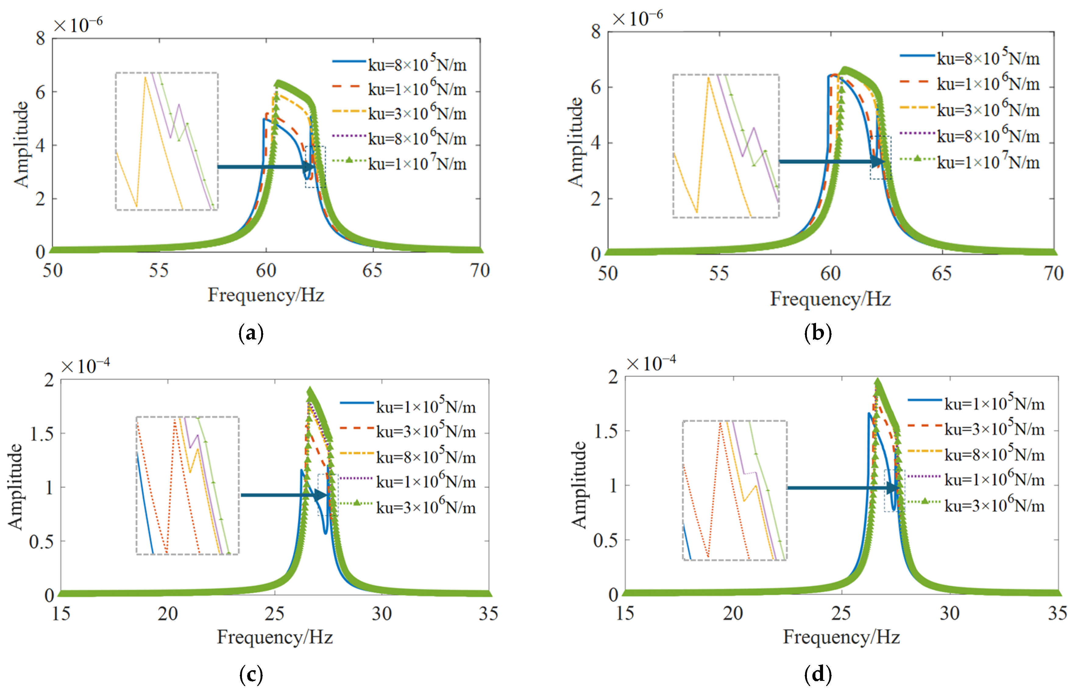
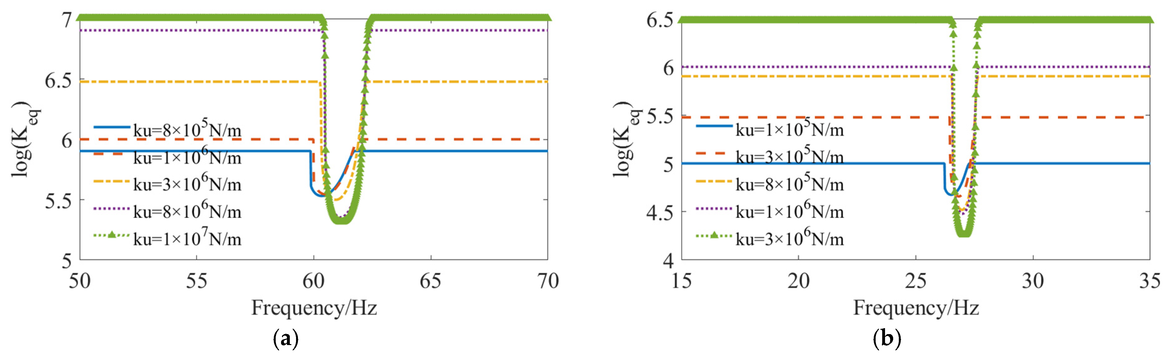
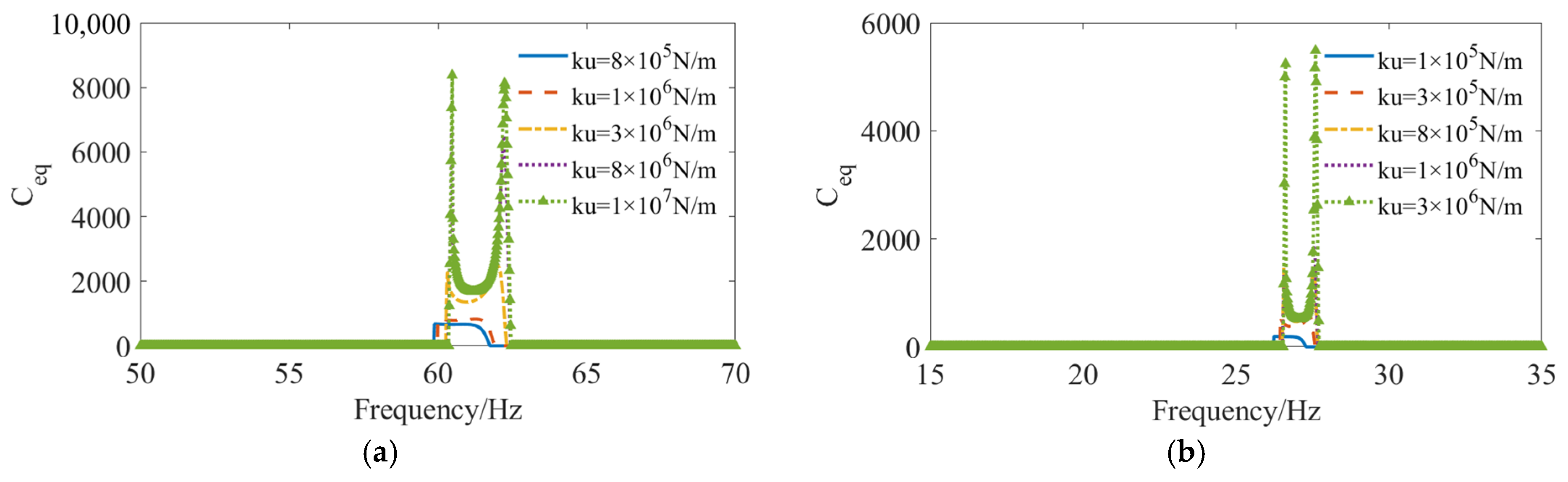
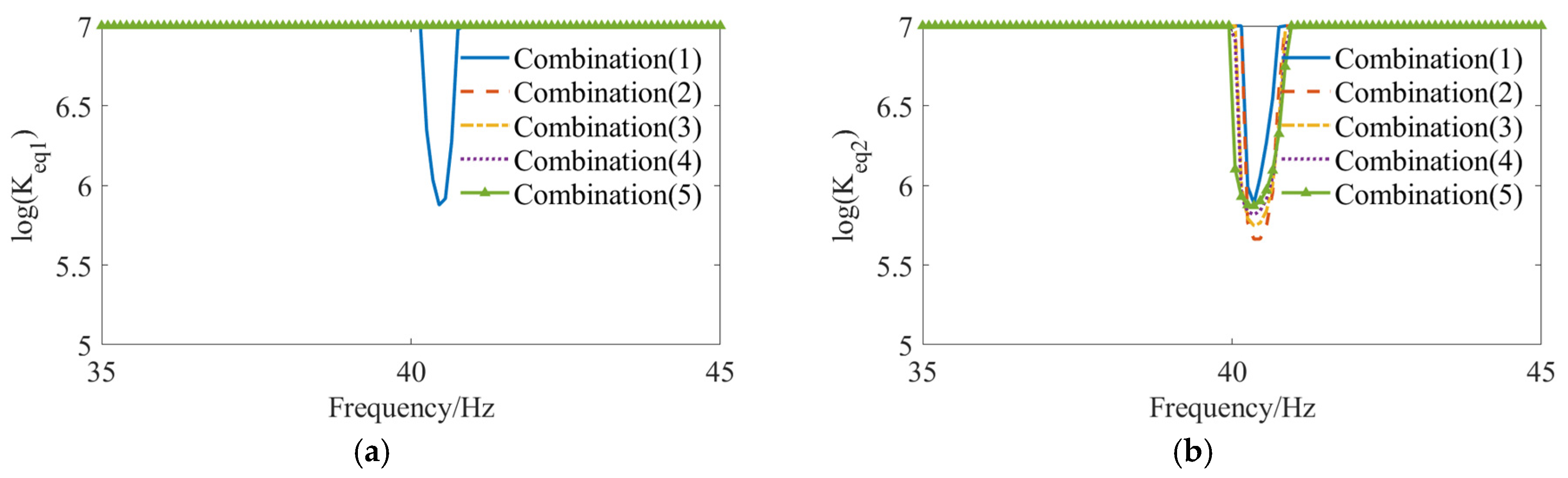
3.4. Different Connection Translation Stiffness

In the process of structural vibration, the connection force in the stick is directly related to the connection stiffness, which will impact the two segments in the connection force segment function (23) and, consequently, influence the connection characteristics of the truss structure. Figure 9 illustrates the frequency response curves of the two sections at the connection point under varying levels of connection stiffness, with an excitation force amplitude of F₀ = 50 N, a preload force of F_N = 500 N, and a friction coefficient of μ = 0.3. Under the influence of greater connection stiffness, the resonance peak is sharp, and the system can be considered as approaching a linear state. At lower stiffness levels, the resonance peaks exhibit increased width and the emergence of two distinct peaks, indicative of internal resonance characteristics in nonlinear systems. Notably, the prominence of these traits increases as stiffness decreases.

In the case of a stiffness of k_u = 8 × 10⁵, where the internal resonance characteristics are more pronounced, Figure 10 illustrates the frequency response as the preload force F_N varies. It can be seen that the internal peak gradually approaches as the preload increases. In the case of simply supported boundary conditions (Figure 10c,d), internal resonance is observed at low preload values; however, this phenomenon diminishes as the preload increases, suggesting a coupled effect between the boundary conditions and the applied load.

The graphs in Figure 11 and Figure 12 illustrate the variation of equivalent stiffness and damping, where the change near the resonance frequency differs greatly from that shown in Figure 4 and Figure 7. As the connection stiffness increases, the magnitude of the equivalent stiffness changes near the resonance frequency is amplified. The resonance frequency wandering is obvious in the case of lower stiffness, thereby reflecting more obvious nonlinear characteristics.

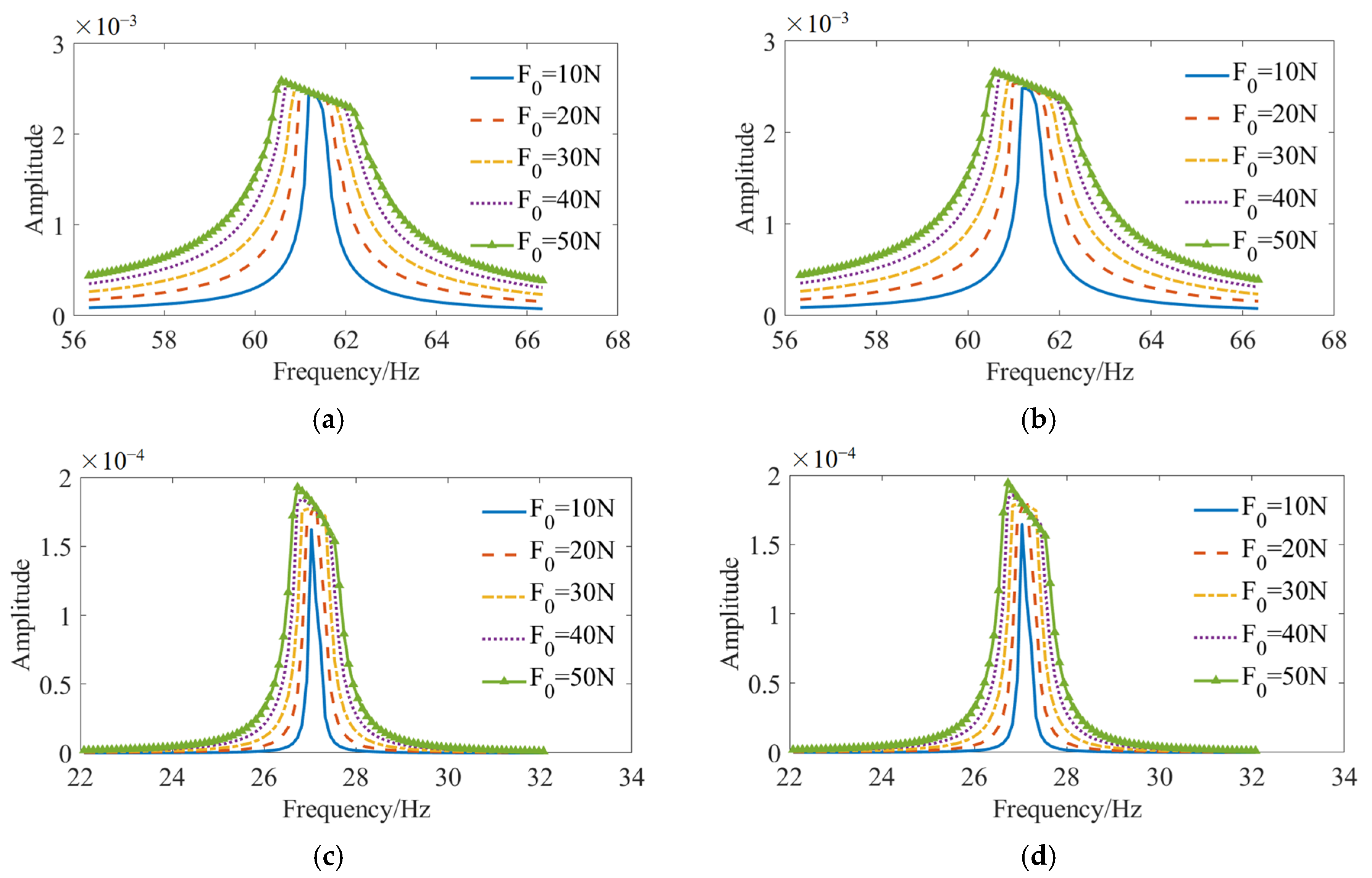
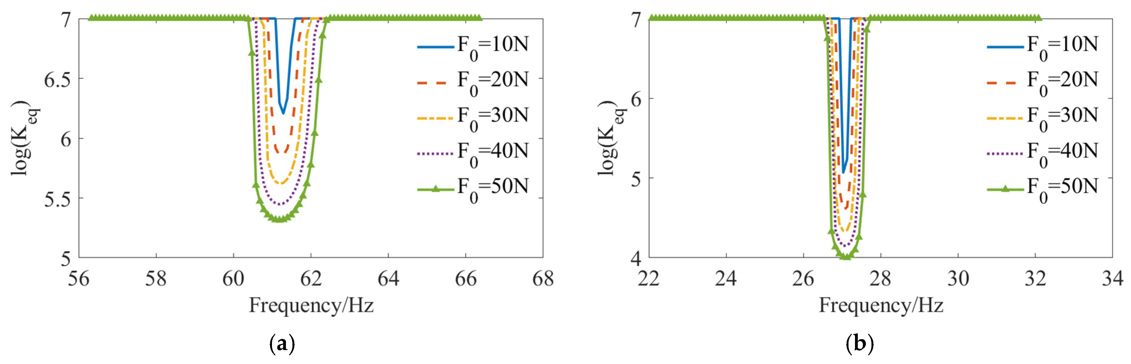
3.5. Effect of Excitation

The connection pressure, friction coefficient, and connection stiffness collectively represent the inherent characteristics of the joint structure, while, besides the above characteristic parameters, changes in the connection state are also related to the magnitude of external excitation. In this section, the influence of excitation on the structural nonlinear vibration response is analyzed. Figure 13 illustrates the structural frequency response curve under different excitation amplitudes, where the connection stiffness and friction coefficient are consistent with Section 3.2, and the connection preload F_N = 500 N.

When the excitation amplitude is small, the resonance peaks in the frequency response curve at both ends of the connection joint are sharp, corresponding to the linear system characteristic of smaller excitations being unable to cause slippage between structures. As the excitation amplitude increases, the resonance peaks become broader, and peak ‘clipping’ occurs, with the highest peak frequency shifting to the left. Under fixed boundary conditions, the resonance frequency range is wider, the ‘clipping’ phenomenon is more obvious, and there is a relatively flat frequency response line. Conversely, under simply supported boundary conditions, there is a more significant difference in equivalent stiffness and damping (as shown in Figure 14 and Figure 15) with changes in excitation, so the peak changes in the frequency response curve are more complex. As the excitation increases, the nonlinear characteristics of the system’s response become more apparent.

3.6. Multi-Beam Situation

The preceding analysis has investigated the nonlinear vibration response of simple structures within a connection model. In practical engineering structures like trusses and beam systems, connection joints may arise in continuous sequences. Therefore, this section will analyze the application of the connection model outlined in this paper within composite structures.

3.6.1. Beams of Different Lengths

Firstly, this summary presents various combinations of beam structures with different lengths and analyzes the frequency response curves of each beam segment, as well as the changing connection state at each connection joint. The total length of the structure is maintained at 1.6 m, including two connection joints and three beams. Considering the comprehensive structural symmetry, the lengths of the beams in the five combinations are as follows: (1) L₁ = 0.6 m, L₂ = 0.4 m, L₃ = 0.6 m; (2) L₁ = 0.65 m, L₂ = 0.4 m, L₃ = 0.55 m; (3) L₁ = 0.7 m, L₂ = 0.4 m, L₃ = 0.5 m; (4) L₁ = 0.75 m, L₂ = 0.4 m, L₃ = 0.45 m; (5) L₁ = 0.8 m, L₂ = 0.4 m, L₃ = 0.4 m. An external excitation force F₀ = 50 N is applied to the midpoint of beam L₂. The preloads F_N1 and F_N2 on the two connection joints are 500 N, the friction coefficients μ₁ = μ₂ = 0.3, the connecting transitional stiffness k_u1 = k_u2 = 1 × 10⁷ N/m, and the connecting rotational stiffness k_θ1 = k_θ2 = 1 × 10⁷ N·m/rad. Three frequency response observation points were selected to be located on their respective segment beams, and the coordinates were P₁: x₁ = 0.4L₁; P₂: x₂ = 0.3L₂; P₃: x₃ = 0.6L₃.

The frequency response curves at each observation point are depicted in Figure 16. It is evident from the figures that variations in the beam length (reflecting the position of the connection joint in the overall structure) significantly impact the structural frequency response curve under external excitation. The response at location P₃ is more sensitive to changes in beam length, indicating a higher sensitivity to the symmetry of the structure, while the response at location P₃ is less affected by variations in the position of the connection joint. When L₁ = L₃, the structure is symmetrical, and it can be observed that the vibration response at each observation point is the ‘sharp’, close to the ideal linear situation. As the length of beam L₁ increases, the overall structure becomes asymmetric, and the vibration response of each observation point is in a straight line within the resonance frequency range.

When the structure is symmetrical (Combination 1), the equivalent stiffness of both joints (Figure 17) decreases by the same amount as the resonance frequency. In contrast, when the structure is asymmetric, the equivalent connection stiffness at the joint between the longer beam L₁ and the intermediate beam L₂ becomes independent of frequency; meanwhile, at the joint on the left side of the shorter beam (L3), there is still a decrease in equivalent stiffness depending on the resonance frequency, with a greater reduction compared to symmetric cases, and the frequency range affected increases with the degree of asymmetry. This suggests that in asymmetrical configurations, the overall structural stiffness diminishes and becomes concentrated towards the joint of the short beam, which plays an important role in predicting changes in structural strength.

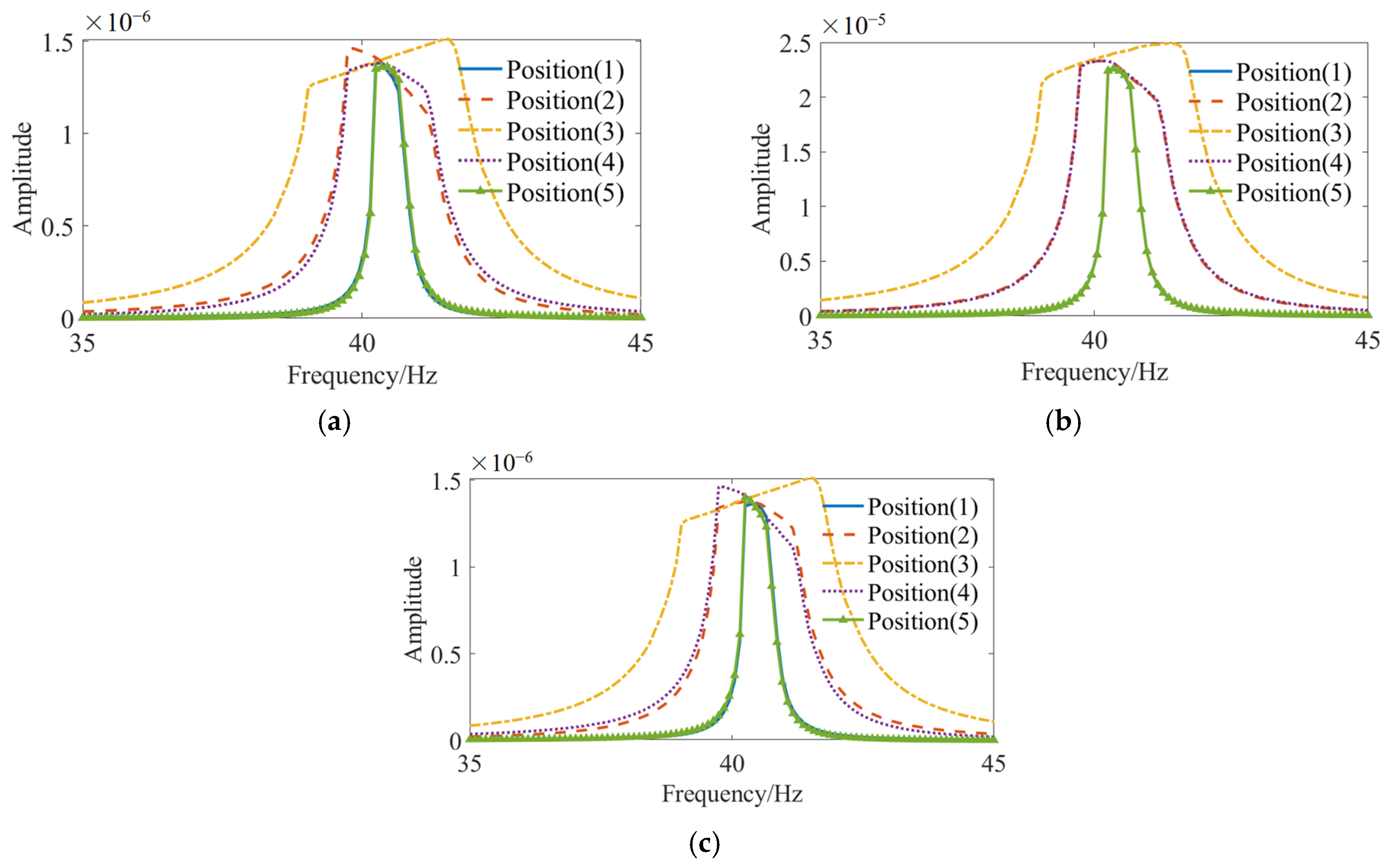
3.6.2. Influence of Excitation Position

Due to the nonlinear connection factors, the position of the applied excitation force will affect the structural transfer matrix, leading to differences in the propagation of elastic waves. Figure 18 illustrates the frequency response curves of the structure under different excitation force application positions. The observation point positions remain consistent with those in Section 3.6.1. The length of each segmented beam is taken from the symmetric case Combination 1 in Section 3.6.1. Five excitation point positions are selected, with the coordinates x₁ = 0.2 m, x₁ = 0.4 m, x₂ = 0.2 m, x₃ = 0.2 m, x₃ = 0.4 m, and the coordinate index indicates which beam the excitation force is acting on. When the excitation force is applied at positions 1 and 5, the modal frequency response curves at each observation point are closest to the linear “sharp” state. Compared to other action positions, positions 1 and 5 are closer to the outer side of the structure, and as the excitation position moves toward the interior of the structure, the resonance frequency range of the frequency response curve increases, and the ‘peak clipping’ becomes more pronounced. From the equivalent stiffness variation curve (Figure 19), the phenomena of the resonance frequency shift and the change in symmetry of the equivalent stiffness are more clearly observable.

4. Conclusions

Aiming to resolve the stick–slip problem that may occur in the connection joints of multi-beam structures, this study employed the Coulomb friction model to develop a vibration analysis framework incorporating contact friction. This framework systematically examines how connection characteristic parameters influence the vibrational behavior of multi-beam structures. Systematic dynamic response analysis yielded the following primary conclusions:

(1)

The alterations in the state of structural connections primarily manifest as a decrease in connection stiffness near the resonance frequency, with the reduction being more pronounced in the simply supported condition than the fixed condition. The “tracking” phenomenon caused by the abrupt change of damping and the variation in resonance frequency results in a relatively stable vibration response amplitude over a larger frequency range.

(2)

As the contact pressure and friction diminish, the frequency response curve progressively flattens, indicating a resonance frequency range. The peak response frequency is observed at the lower end of this resonance range, which is situated below the linear natural frequency.

(3)

When the connection stiffness is reduced, the resonance peaks broaden and diverge, exhibiting the characteristics of internal resonance in nonlinear systems. This feature becomes increasingly pronounced as the stiffness decreases.

(4)

The magnitude of external excitation serves as a direct factor in inducing nonlinear softening of the connection. When the excitation amplitude is minimal, its impact on the connection state remains limited. As the external excitation escalates, the structure’s frequency response curve exhibits a resonance region.

(5)

Various sub-beam combinations display distinct nonlinear characteristics when used in multi-beam structures. In asymmetric configurations, alterations in connection states are primarily induced by excitation and predominantly manifest at the junctions of shorter beams. As the excitation point approaches the structural center, it is more likely to cause significant changes in connection states, thereby broadening the range of resonant intervals.

References

1. Han, S.M.; Benaroya, H.; Wei, T. Dynamics of transversely vibrating beams using four engineering theories. J. Sound Vib. 1999, 225, 935–988. [Google Scholar] [CrossRef]
2. Timoshenko, S. History of Strength of Materials: With a Brief Account of the History of Theory of Elasticity and Theory of Structures; Courier Corporation: Chelmsford, MA, USA, 1983. [Google Scholar]
3. Timoshenko, S.P.X. On the transverse vibrations of bars of uniform cross-section. Lond. Edinb. Dublin Philos. Mag. J. Sci. 1922, 43, 125–131. [Google Scholar] [CrossRef]
4. Strutt, J.W.; Rayleigh, J.W.S. The Theory of Sound; Macmillan: London, UK, 1877; Volume 1. [Google Scholar]
5. Abbas, B.A.H.; Thomas, J. The second frequency spectrum of Timoshenko beams. J. Sound Vib. 1977, 51, 123–137. [Google Scholar] [CrossRef]
6. Mao, Q.; Pietrzko, S. Free vibration analysis of stepped beams by using Adomian decomposition method. Appl. Math. Comput. 2010, 217, 3429–3441. [Google Scholar] [CrossRef]
7. Kiani, K.; Soltani, S. Nonlocal longitudinal, flapwise, and chordwise vibrations of rotary doubly coaxial/non-coaxial nanobeams as nanomotors. Int. J. Mech. Sci. 2020, 168, 105291. [Google Scholar] [CrossRef]
8. Guler, S. Free vibration analysis of a rotating single edge cracked axially functionally graded beam for flap-wise and chord-wise modes. Eng. Struct. 2021, 242, 112564. [Google Scholar] [CrossRef]
9. Banerjee, J.R. Dynamic stiffness formulation and free vibration analysis of centrifugally stiffened Timoshenko beams. J. Sound Vib. 2001, 247, 97–115. [Google Scholar] [CrossRef]
10. Shu, C. Differential Quadrature and Its Application in Engineering; Springer Science & Business Media: Berlin/Heidelberg, Germany, 2012. [Google Scholar]
11. Bazoune, A. Effect of tapering on natural frequencies of rotating beams. Shock Vib. 2007, 14, 169–179. [Google Scholar] [CrossRef]
12. Bograd, S.; Reuss, P.; Schmidt, A.; Gaul, L.; Mayer, M. Modeling the dynamics of mechanical joints. Mech. Syst. Signal Process. 2011, 25, 2801–2826. [Google Scholar] [CrossRef]
13. Sun, D.; Li, W.Y.; Lyu, B.L. Overview of mechanical modeling methods for bolted connections. J. Vib. Acoust. 2012, 32, 8–12. [Google Scholar]
14. Iwan, W.D. A distributed-element model for hysteresis and its steady-state dynamic response. J. Appl. Mech. 1966, 33, 893–900. [Google Scholar] [CrossRef]
15. Iwan, W.D. On a class of models for the yielding behavior of continuous and composite systems. J. Appl. Mech. 1966, 34, 612–617. [Google Scholar] [CrossRef]
16. An, W.W.; Gong, Z.R.; Zhao, T. Dynamic Properties of Machine Bolted Joints Summary. Appl. Mech. Mater. 2013, 423, 1594–1602. [Google Scholar] [CrossRef]
17. Valanis, K.C. Fundamental consequences of a new intrinsic time measure: Plasticity as a limit of the endochronic theory. Arch. Mech. Stossowanej 1980, 32, 171–191. [Google Scholar]
18. Bouc, R. Forced vibrations of mechanical systems with hysteresis. In Proceedings of the Fourth Conference on Nonlinear Oscillations, Prague, Czech Republic, 5–9 September 1967. [Google Scholar]
19. Wen, Y.K. Method for random vibration of hysteretic systems. J. Eng. Mech. Div. 1976, 102, 249–263. [Google Scholar] [CrossRef]
20. Kim, J.; Yoon, J.C.; Kang, B.S. Finite element analysis and modelling of structure with bolted joints. Appl. Math. Model. 2007, 31, 895–911. [Google Scholar] [CrossRef]
21. Qin, Z.; Han, Q.; Chu, F. Bolt loosening at rotating joint interface and its influence on rotor dynamics. Eng. Fail. Anal. 2016, 59, 456–466. [Google Scholar] [CrossRef]
22. Rao, C.K.; Mirza, S. A note on vibrations of generally restrained beams. J. Sound Vib. 1989, 130, 453–465. [Google Scholar] [CrossRef]
23. Kim, H.K.; Kim, M.S. Vibration of beams with generally restrained boundary conditions using Fourier series. J. Sound Vib. 2001, 245, 771–784. [Google Scholar] [CrossRef]
24. Abbas, B.A.H. Vibrations of Timoshenko beams with elastically restrained ends. J. Sound Vib. 1984, 97, 541–548. [Google Scholar] [CrossRef]
25. Elishakoff, I.; Lin, Y.K.; Zhu, L.P. Random vibration of uniform beams with varying boundary conditions by the dynamic-edge-effect method. Comput. Methods Appl. Mech. Eng. 1995, 121, 59–76. [Google Scholar] [CrossRef]
26. Li, X.Y.; Zhao, X.; Li, Y.H. Green’s functions of the forced vibration of Timoshenko beams with damping effect. J. Sound Vib. 2014, 333, 1781–1795. [Google Scholar] [CrossRef]
27. Li, W.L. Free vibrations of beams with general boundary conditions. J. Sound Vib. 2000, 237, 709–725. [Google Scholar] [CrossRef]
28. Copetti, R.D.; Claeyssen, J.R.; de Rosso Tolfo, D.; Pavlack, B.S. The fundamental modal response of elastically connected parallel Timoshenko beams. J. Sound Vib. 2022, 530, 116920. [Google Scholar] [CrossRef]
29. Wu, Z.; Wang, Y.; Li, B.; Wen, B.; Ma, Q. Analysis of natural vibration characteristics of continuous multi-span beams with concentrated mass under arbitrary boundary conditions. J. Vib. Acoust. 2024, 44, 52–58+85. [Google Scholar]
30. Hao, Q.; Zhai, W.; Chen, Z. Free vibration of connected double-beam system with general boundary conditions by a modified Fourier–Ritz method. Arch. Appl. Mech. 2018, 88, 741–754. [Google Scholar] [CrossRef]
31. Li, W.L.; Xu, H. An exact fourier series method for the vibration analysis of multispan beam systems. J. Comput. Nonlinear Dyn. 2009, 4, 710–733. [Google Scholar] [CrossRef]
32. Couch, L.; Tehrani, F.M.; Naghshineh, A.; Frazao, R. Shake Table response of a dual system with inline friction damper. Eng. Struct. 2023, 281, 115776. [Google Scholar] [CrossRef]
33. Li, Y.; Long, T.; Luo, Z.; Wen, C.; Zhu, Z.; Jin, L.; Li, B. Numerical and experimental investigations on dynamic behaviors of a bolted joint rotor system with pedestal looseness. J. Sound Vib. 2024, 571, 118036. [Google Scholar] [CrossRef]
34. Kang, B.; Tan, C.A. Nonlinear response of a beam under distributed moving contact load. Commun. Nonlinear Sci. Numer. Simul. 2006, 11, 203–232. [Google Scholar] [CrossRef]
35. Sinou, J.J.; Dereure, O.; Mazet, G.B.; Thouverez, F.; Jezequel, L. Friction-induced vibration for an aircraft brake system-Part 1: Experimental approach and stability analysis. Int. J. Mech. Sci. 2006, 48, 536–554. [Google Scholar] [CrossRef]
36. Joglekar, D.M. Analysis of nonlinear frequency mixing in Timoshenko beams with a breathing crack using wavelet spectral finite element method. J. Sound Vib. 2020, 488, 115532. [Google Scholar] [CrossRef]
37. Zhao, Y.; Du, J. Nonlinear vibration analysis of a generally restrained double-beam structure coupled via an elastic connector of cubic nonlinearity. Nonlinear Dyn. 2022, 109, 563–588. [Google Scholar] [CrossRef]
38. Krack, M.; Bergman, L.A.; Vakakis, A.F. On the efficacy of friction damping in the presence of nonlinear modal interactions. J. Sound Vib. 2016, 370, 209–220. [Google Scholar] [CrossRef]
39. Tüfekci, M.; Sun, Y.; Yuan, J.; Maharaj, C.; Liu, H.; Dear, J.P.; Salles, L. Analytical vibration modelling and solution of bars with frictional clamps. J. Sound Vib. 2024, 577, 118307. [Google Scholar] [CrossRef]
40. Tang, Q.; Li, C.; She, H.; Wen, B. Nonlinear response analysis of bolted joined cylindrical-cylindrical shell with general boundary condition. J. Sound Vib. 2019, 443, 788–803. [Google Scholar] [CrossRef]
41. Lu, K.; Jin, Y.; Chen, Y.; Cao, Q.; Zhang, Z. Stability analysis of reduced rotor pedestal looseness fault model. Nonlinear Dyn. 2015, 82, 1611–1622. [Google Scholar] [CrossRef]
42. Lu, K.; Cheng, H.; Zhang, W.; Zhang, H.; Zhang, K.; Fu, C. Nonlinear dynamic behavior of a dual-rotor bearing system with coupling misalignment and rubbing faults. Meas. Sci. Technol. 2022, 34, 014005. [Google Scholar]
43. Casini, P.; Vestroni, F. Mitigation of Structural Vibrations of MDOF Oscillators by Modal Coupling Due to Hysteretic Dampers. Appl. Sci. 2022, 12, 10079. [Google Scholar] [CrossRef]
44. Jewell, E.; Allen, M.S.; Zare, I.; Wall, M. Application of quasi-static modal analysis to a finite element model and experimental correlation. J. Sound Vib. 2020, 479, 115376. [Google Scholar] [CrossRef]
45. Zang, J.; Yuan, T.C.; Lu, Z.Q.; Zhang, Y.W.; Ding, H.; Chen, L.Q. A lever-type nonlinear energy sink. J. Sound Vib. 2018, 437, 119–134. [Google Scholar] [CrossRef]
46. Dai, W.; Yang, J.; Wiercigroch, M. Vibration energy flow transmission in systems with Coulomb friction. Int. J. Mech. Sci. 2022, 214, 106932. [Google Scholar] [CrossRef]
47. Alberto, J.; Fuentes, A. On the Influence of Piecewise Defined Contact Geometries on Friction Dampers; KIT Scientific Publishing: Karlsruhe, Germany, 2023; p. 182. [Google Scholar]
48. Riddoch, D.J.; Cicirello, A.; Hills, D.A. Response of a mass-spring system subject to Coulomb damping and harmonic base excitation. Int. J. Solids Struct. 2020, 193, 527–534. [Google Scholar] [CrossRef]
49. Marino, L.; Cicirello, A.; Hills, D.A. Displacement transmissibility of a Coulomb friction oscillator subject to joined base-wall motion. Nonlinear Dyn. 2019, 98, 2595–2612. [Google Scholar] [CrossRef]
50. Marino, L.; Cicirello, A. Experimental investigation of a single-degree-of-freedom system with Coulomb friction. Nonlinear Dyn. 2020, 99, 1781–1799. [Google Scholar] [CrossRef]
51. Marino, L.; Cicirello, A. Multi-degree-of-freedom systems with a Coulomb friction contact: Analytical boundaries of motion regimes. Nonlinear Dyn. 2021, 104, 35–63. [Google Scholar] [CrossRef]
52. Asadi, K.; Ahmadian, H.; Jalali, H. Micro/macro-slip damping in beams with frictional contact interface. J. Sound Vib. 2012, 331, 4704–4712. [Google Scholar] [CrossRef]
53. Won, H.I.; Chung, J. Numerical analysis for the stick-slip vibration of a transversely moving beam in contact with a frictional wall. J. Sound Vib. 2018, 419, 42–62. [Google Scholar] [CrossRef]
54. Won, H.I.; Lee, B.; Chung, J. Stick-slip vibration of a cantilever beam subjected to harmonic base excitation. Nonlinear Dyn. 2018, 92, 1815–1828. [Google Scholar] [CrossRef]
55. Baek, S.; Epureanu, B. Reduced-order modeling of bladed disks with friction ring dampers. J. Vib. Acoust. 2017, 139, 061011. [Google Scholar] [CrossRef]
Figure 1. A beam structure model considering connection. The length of the beam is Li; the translational and rotational stiffness levels of the constraints at the edges are kl1, kl2, kr1, and kr2; and the connection stiffness levels at the joints are kui and kθi, respectively.
Applsci 15 01141 g001
Figure 2. The experimental test system and two composite beam structures are presented. (a) The experimental setup; (b) Case I, beam structure dimensions: L1 = 340 mm, L2 = 340 mm; (c) Case II, beam structure dimensions: L1 = 425 mm, L2 = 255 mm.
Applsci 15 01141 g002
Figure 3. Frequency response curves under different preload conditions. (a) Fixed support boundary, L1 connection point; (b) fixed support boundary, L2 connection point; (c) simply supported boundary, L1 connection point; (d) simply supported boundary, L2 connection point.
Applsci 15 01141 g003
Figure 4. Curves of equivalent stiffness and excitation frequency under different bolt preload conditions. (a) Fixed support boundary; (b) simply supported boundary.
Applsci 15 01141 g004
Figure 5. Curves of equivalent damping and excitation frequency under different bolt preload conditions. (a) Fixed support boundary; (b) simply supported boundary.
Applsci 15 01141 g005
Figure 6. Frequency response curves with different friction coefficients. (a) Fixed support boundary, L1 connection point; (b) fixed support boundary, L2 connection point; (c) simply supported boundary, L1 connection point; (d) simply supported boundary, L2 connection point.
Applsci 15 01141 g006
Figure 7. The curves of equivalent stiffness and excitation frequency under different friction coefficients. (a) Fixed support boundary; (b) simply supported boundary.
Applsci 15 01141 g007
Figure 8. The curves of equivalent damping and excitation frequency under different friction coefficients. (a) Fixed support boundary; (b) simply supported boundary.
Applsci 15 01141 g008
Figure 9. Frequency response curves with different connection stiffness conditions. (a) Fixed support boundary, L1 connection point; (b) fixed support boundary, L2 connection point; (c) simply supported boundary, L1 connection point; (d) simply supported boundary, L2 connection point.
Applsci 15 01141 g009
Figure 10. Variations in the frequency response curves due to preload force. (a) Fixed support boundary, L1 connection point; (b) fixed support boundary, L2 connection point; (c) simply supported boundary, L1 connection point; (d) simply supported boundary, L2 connection point.
Applsci 15 01141 g010
Figure 11. The relationship between equivalent stiffness and excitation frequency under different levels of connection stiffness. (a) Fixed support boundary; (b) simply supported boundary.
Applsci 15 01141 g011
Figure 12. The relationship between equivalent damping and excitation frequency under different levels of connection stiffness. (a) Fixed support boundary; (b) simply supported boundary.
Applsci 15 01141 g012
Figure 13. Frequency response curves under different excitation amplitudes. (a) Fixed support boundary, L1 connection point; (b) fixed support boundary, L2 connection point; (c) simply supported boundary, L1 connection point; (d) simply supported boundary, L2 connection point.
Applsci 15 01141 g013
Figure 14. The curves of equivalent stiffness and excitation frequency under different excitation amplitudes. (a) Fixed support boundary; (b) simply supported boundary.
Applsci 15 01141 g014
Figure 15. The curves of equivalent damping and excitation frequency under different excitation amplitudes. (a) Fixed support boundary; (b) simply supported boundary.
Applsci 15 01141 g015
Figure 16. The amplitude–frequency curves of the observation points with different length combinations, for which the coordinates were (1) L1 = 0.6 m, L2 = 0.4 m, L3 = 0.6 m; (2) L1 = 0.65 m, L2 = 0.4 m, L3 = 0.55 m; (3) L1 = 0.7 m, L2 = 0.4 m, L3 = 0.5 m; (4) L1 = 0.75 m, L2 = 0.4 m, L3 = 0.45 m; (5) L1 = 0.8 m, L2 = 0.4 m, L3 = 0.4 m. (a) P1: x1 = 0.4L1; (b) P2: x2 = 0.3L2; (c) P3: x3 = 0.6L3.
Applsci 15 01141 g016
Figure 17. The changes in the equivalent stiffness of the connections under different length combinations, for which the coordinates were (1) L1 = 0.6 m, L2 = 0.4 m, L3 = 0.6 m; (2) L1 = 0.65 m, L2 = 0.4 m, L3 = 0.55 m; (3) L1 = 0.7 m, L2 = 0.4 m, L3 = 0.5 m; (4) L1 = 0.75 m, L2 = 0.4 m, L3 = 0.45 m; (5) L1 = 0.8 m, L2 = 0.4 m, L3 = 0.4 m. (a) Joint 1; (b) joint 2.
Applsci 15 01141 g017
Figure 18. The frequency amplitude curves of each observation point at different excitation positions, for which the coordinates were (1) x1 = 0.2 m, (2) x1 = 0.4 m, (3) x2 = 0.2 m, (4) x3 = 0.2 m, (5) x3 = 0.4 m. (a) P1: x1 = 0.4L1; (b) P2: x2 = 0.3L2; (c) P3: x3 = 0.6L3.
Applsci 15 01141 g018
Figure 19. The changes in the equivalent stiffness of the connection at different excitation positions, for which the coordinates were (1) x1 = 0.2 m, (2) x1 = 0.4 m, (3) x2 = 0.2 m, (4) x3 = 0.2 m, (5) x3 = 0.4 m. (a) Joint 1; (b) joint 2.
Applsci 15 01141 g019