1. Introduction
In recent years, the global surge in e-commerce adoption has significantly influenced distribution and last-mile delivery logistics. Last-mile delivery logistics denote the final phase of a product’s delivery process, bringing it to the end customer. This stage has become a focal point in logistics strategies due to its critical influence on customer satisfaction, delivery speed, cost efficiency, and overall convenience. Over the past decade, electric vehicles (EVs) have become prevalent in last-mile delivery services due to their capacity to reduce greenhouse gas emissions, support renewable energy, and establish sustainable transportation systems. The benefits of EVs include decreased transportation costs, enhanced energy efficiency, and significantly reduced pollutant emissions. With the increasing use of EVs, the routing problem of these vehicles has emerged. The problem is known as the Electric Vehicle Routing Problem (EVRP) in the literature. The primary difference between the EVRP and the classic VRP is that vehicles have a battery as an energy source, and the charge level decreases as the vehicle travels on the road. Consequently, the EVRP places substantial emphasis on accounting for charging capacities and the strategic placement of charging stations, as these factors are crucial for the efficient operation of an EV fleet. A common constraint across all EVRP variations is the necessity to visit a recharging station due to the limited driving range of electric vehicles. In traditional Vehicle Routing Problems (VRPs), gas and diesel vehicles typically have longer ranges, enabling them to travel hundreds of kilometers on a single refuel. Refueling needs arise less frequently in daily route planning. Additionally, refueling durations generally range between 5 and 10 min, which does not substantially impact the overall travel time of the route. The widespread distribution of gas and diesel stations, extending from urban centers to rural areas, further mitigates the necessity to incorporate refueling points within route planning models. Conversely, within the framework of the EVRP, the integration of charging stations into routes becomes imperative due to the limited battery capacity and comparatively prolonged charging times of electric vehicles. Electric vehicles must recharge at specific intervals to address range limitations, and the strategic placement of charging stations directly influences this process. Consequently, the EVRP presents a more complex modeling challenge than the classical VRP, as it necessitates considering charging times and station visit decisions as additional variables in route planning. The decision to include charging station visits emerges as a critical component in the context of the EVRP.
In this paper we address the Capacitated Electric Vehicle Routing Problem (CEVRP). The CEVRP aims to address operational and environmental objectives by accounting for electric vehicles’ limited driving range and load capacities. Including capacity constraints facilitates more realistic industrial planning. CEVRP-based strategies promote environmental sustainability and reduce operational costs by optimizing routes for energy efficiency and minimizing carbon emissions. A fleet management that produces fewer emissions and considers energy efficiency supports corporate environmental policies. As a result, the CEVRP has been increasingly adopted in today’s last-mile delivery operations, leading the way for broader implementation of eco-friendly solutions in the logistics sector.
Since the VRP is an NP-hard problem and the EVRP is a generalization of the VRP, the EVRP can equally be considered NP-hard in the strong sense [
1]. Solution methodologies proposed in the literature for addressing the EVRP and its variants can be categorized into exact solution methods, heuristic methods, metaheuristic methods, and learning-based methods [
2,
3,
4,
5,
6,
7]. Due to the problem’s complexity, exact methods either fail to provide solutions for large-scale instances or require excessive computational time. Consequently, researchers have proposed heuristic and metaheuristic methods to address these challenges. While these methods do not guarantee optimal solutions, they produce high-quality solutions within a reasonable time frame [
8,
9,
10]. In recent years, studies incorporating self-learning methods, a sub-branch of machine learning, have gained prominence. The models and solutions developed for classical vehicle routing cannot be directly applied to electric vehicles. Additionally, the need to study learning-based Vehicle Routing Problems specifically for electric vehicles and propose effective solutions has become increasingly important. In the last few years, research integrating self-learning methodologies has gained considerable prominence, with deep reinforcement learning (DRL) emerging as a key focus in the study of Vehicle Routing Problems [
4,
5,
6,
7]. Reinforcement learning methods involve strategies whereby agents determine the optimal course of action based on the state or observation of the environment. The agent selects actions from a set of available options and receives rewards based on the utility of the actions taken within a given time step. The actions chosen by the agent can alter the state of the environment in which it operates.
EVRP softwares are crucial in supporting daily operational decisions within the logistics and distribution sectors. These decisions encompass route planning, vehicle assignment, charging station selection, and real-time updates. Typically, these processes are initiated at various times of day and should be completed quickly and efficiently. As a realistic decision-making time, algorithms should produce results approximately within 2 min for a medium-size last-mile delivery problem [
11]. Reinforcement learning (RL) methods enhance the effectiveness of EVRP softwares by enabling the generation of solutions more rapidly compared to traditional optimization methods. This capability for rapid solution production significantly increases the practical applicability of RL algorithms, particularly given the dynamic nature of logistics operations. The ability of RL approaches to produce fast and adaptive solutions aligns well with the operational requirements of logistics, where timely and flexible decision making is essential for maintaining efficiency and meeting service standards.
Upon reviewing the EVRP literature on the application of Q-learning, two notable studies emerge. The study of Ottoni et al. [
12] employs reinforcement learning to address the Electric Vehicle Traveling Salesman Problem (EVTSP), comparing the performance of two reinforcement learning algorithms, Q-learning and SARSA. The study provides route optimization for a single electric vehicle. This approach does not incorporate the management of multiple electric vehicles, which is essential for addressing fleet-based scenarios such as the CEVRP. Consequently, the methodology is not directly transferable to multi-vehicle contexts. The second study [
13] is focused on generating energy-efficient routes for electric vehicles from a source to a destination while considering the possibility of recharging at intermediate charging stations. The studies of the path planning include tasks from a point (source) to another point (destination). In these studies, the most suitable route between two points is obtained and there is no obligation to go to any point other than the start–end points. However, in the last-mile delivery, there is a need for multi-delivery tasks for transportation. This approach overlooks critical constraints, such as the load capacity of the vehicles [
14]. As a result, the method is not directly applicable to CEVRP, which necessitates the consideration of multi-task constraints.
In this study we propose a Q-learning method specifically designed to solve the CEVRP, incorporating well-defined reward structures and fine-tuned hyperparameters for enhanced performance. In this study, route planning is conducted for multiple EVs. However, the number of vehicles is not predetermined at the outset; instead, it is dynamically determined based on customer demand and route optimization. Routes are found where all customer demands are met and the total distance traveled by the fleet is minimized. The number of EVs in the solution is suggested and optimized by the model as in the study [
2,
4]. This means that a smaller number of EVs will not be enough for customers’ demands and a higher number will be excessive and lead to unnecessary energy consumption. In the proposed method, a single-agent approach is adopted to jointly determine both the routes and the number of EVs within an integrated framework, rather than conducting independent planning processes for each EV.
To the best of our knowledge, this study is pioneering work using a Q-learning algorithm to solve the CEVRP. The proposed algorithm is tested using a newly presented dataset. The dataset is based on real-world data, thereby addressing a notable gap in the literature, where datasets for the EVRP and its variants are predominantly derived from synthetic data. Synthetic datasets frequently fail to capture the full complexity and intricacies of real-world logistics problems. The existing datasets for the EVRP in the literature typically consist of customer coordinates (x, y), with distances between nodes calculated using the Euclidean distance metric. However, methods that utilize environmental data, such as reinforcement learning, require additional information related to the environment, including streets, intersections, and traffic density. RL is a general method and can work with any data; however, to correctly model the state transitions in the environment, access to environmental data such as street structure, intersection information, and traffic status often plays a more critical role in these approaches. Therefore, the “need to use environmental data” is not a requirement specific to RL; however, since the definitions of “state” and “reward” in RL are directly shaped by environmental factors, the richer these data are, the higher the learning process and decision quality tend to be. Consequently, the richness and quality of the environmental data directly enhance the learning process and the resulting decision-making quality.
Optimal solutions for this dataset are obtained through a mathematical model that addresses the CEVRP, where each EV has a limited cargo load and battery capacity to satisfy customers’ delivery demands within specified time windows. Experimental results demonstrate that the proposed algorithm achieves near-optimal solutions in a short time for large-scale test problems.
The contributions of this study to the literature can be summarized as follows:
A dataset fulfilling the ’environment’ requirement for researchers working on the EVRP using reinforcement learning is provided.
Optimal solutions are presented for scenarios with and without time windows (TW) in the dataset generated from a last-mile delivery perspective.
A solution to the CEVRP problem using Q-learning is proposed, and comparisons are made with the mathematical model.
The remainder of the paper is organized as follows:
Section 2 reviews the literature on related problems and presents the place of the subject in the literature.
Section 3 outlines the definitions and steps involved in generating the dataset. In
Section 4, the CEVRPTW problem is defined, and the corresponding mathematical model is introduced.
Section 5 provides a detailed explanation of the Q-learning method developed to address this problem.
Section 6 presents computational experiments and analysis. Finally,
Section 7 concludes the paper and discusses future research directions.
2. Literature Review
The EVRP is in the NP-hard problem class. Various approaches have been employed by researchers to address this problem, including exact solution methods, heuristic methods, metaheuristic methods, and learning-based techniques. A summary of the advantages and disadvantages associated with each of these methodologies is provided in
Table 1.
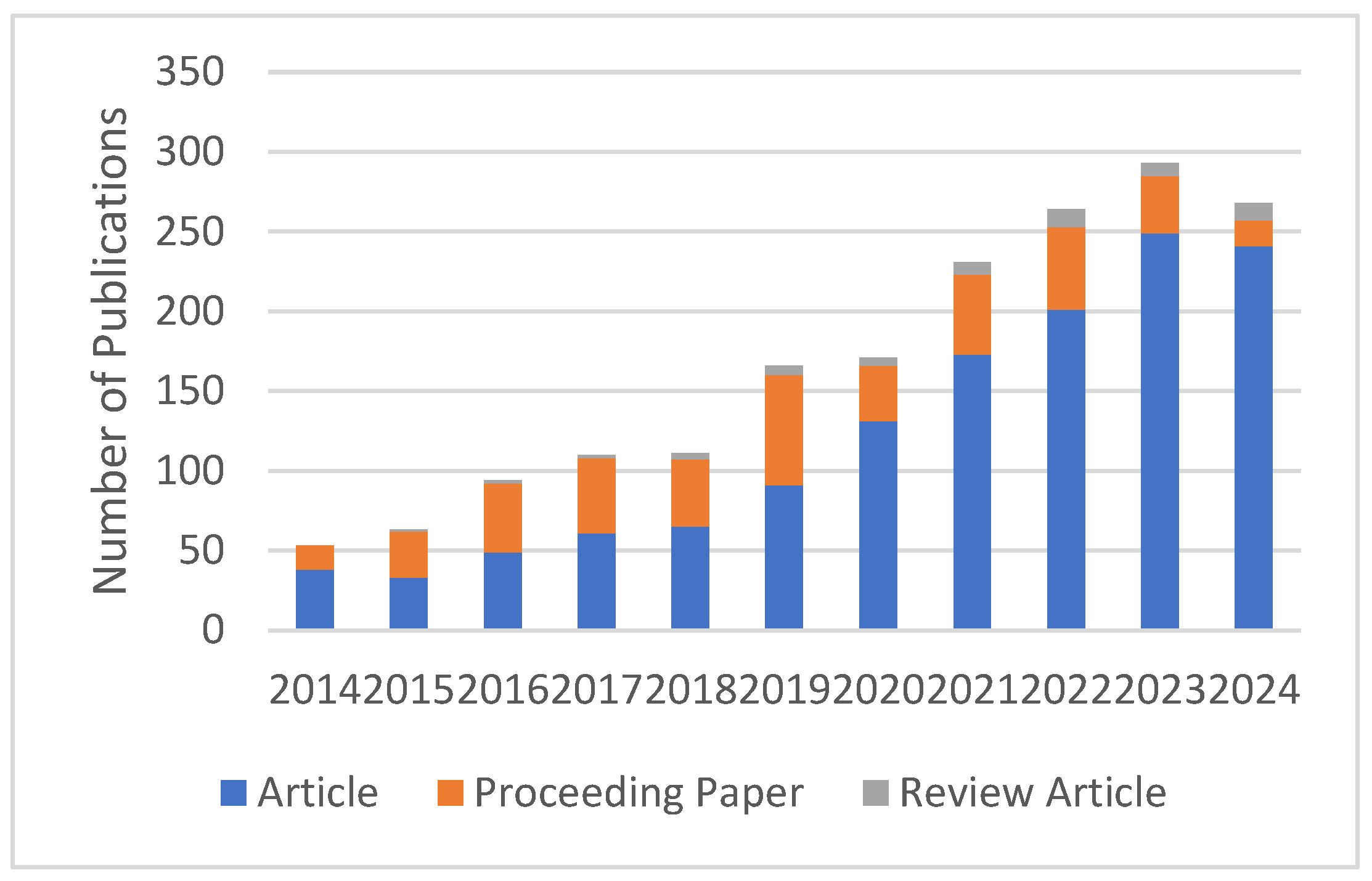
The number of publications regarding the EVRP on the Web of Science (WOS) between 2014 and 2024 is shown in
Figure 1. To obtain
Figure 1, the WOS database was searched with the query “ALL = “electric vehicle” AND (ALL = route planning OR ALL = path planning OR ALL = task scheduling OR ALL = routing)”. This query included all papers that contained the phrase “electric vehicle” and also contained at least one of the phrases “route planning”, “path planning”, “task scheduling”, or “routing”. It seems that interest in the subject has increased in recent years.
There are review and survey studies on the EVRP and its variants in the literature [
1,
30,
31,
32,
33]. Erdelic and Caric [
30] present a literature review on the latest developments regarding the EVRP. This study provides an overview of state-of-the-art procedures for solving the EVRP and related problems. The study of Qin et al. [
31] presents comprehensive research on EV routing problems and their many types. In the study, EV routing problems are divided into nine classes. For each of these nine classes, the settings of the problem variables and the algorithms used to obtain their solutions are examined.
Many researchers have used algorithms that give exact solutions (branch-and-cut algorithms, branch-and-price algorithms, branch-and-price-and-cut algorithms) for the solution of the EVRP and its variants in the literature [
15,
16,
17,
18]. The study of Desaulniers et al. [
15] considers four variants of the problem: (i) at most, a single charge is allowed per route, and the batteries are fully charged during the visit to a charging station; (ii) more than one charge per route (full charging only); (iii) a maximum of one single charge (partial charging). Exact branch-price-and-cut algorithms are presented to generate suitable vehicle routes. Computational results show all four variants are solvable—for instance, with up to 100 customers and 21 charging stations. Keskin and Catay [
16] discuss the EVRPTW and model this problem by allowing partial charges with three charging configurations: normal, fast, and super-fast. The study aims to minimize the total charging cost while operating a minimum number of vehicles. The problem is formulated as a Mixed Integer Linear Program (MILP), and small instances are solved using the CPLEX solver. The Adaptive Large Neighborhood Search (ALNS) is combined with an exact method to solve large instances. In the Lam et al. [
17] study, a branch-and-cut-and-price algorithm is proposed for the Electric Vehicle Routing Problem, with time windows, piecewise-linear recharging, and capacitated recharging stations. The proposed algorithm decomposes the routing to integer programming and the scheduling to constraint programming. Results show that this hybrid algorithm solves instances with up to 100 customers.
Some studies in the literature aim to solve problems with heuristic or metaheuristic methods [
8,
9,
10,
19,
20,
21,
22,
23]. Jia et al. [
8] propose a novel bi-level Ant Colony Optimization algorithm to solve the CEVRP. The study involves finding optimal routes for a fleet of electric vehicles to serve customers while satisfying capacity and electricity constraints. The algorithm treats the CEVRP as a bi-level optimization problem by dividing it into two sub-problems: the upper-level Capacitated Vehicle Routing Problem (CVRP) and the lower-level Fixed Route Vehicle Charging Problem (FRVCP). Akbay et al. [
9] propose a modified Clarke and Wright Savings Heuristic for the EVRPTW. The solutions of the heuristic serve as initial solutions for the Variable Neighborhood Search metaheuristic. Numerical results show that the Variable Neighborhood Search matches the CPLEX in the small problems. The study of Rastani and Catay [
10] mentions that cargo weight plays an important role in routing electric vehicles as it can significantly affect energy consumption. The Large Neighborhood Search method, a metaheuristic algorithm, has been proposed to solve the problem. The study shows that cargo weight can create significant changes in route plans and fleet size and neglecting it can cause severe disruptions in service and increase costs. Deng et al. [
21] introduce an Improved Differential Evolution (IDE) algorithm to address a variant of the EVRP that includes time windows and a partial charge policy with nonlinear charging. The proposed algorithm is compared with the genetic algorithm, artificial bee colony algorithm, and Adaptive Large Neighborhood Search for comparison. Experimental comparisons reveal that the IDE is superior to others.
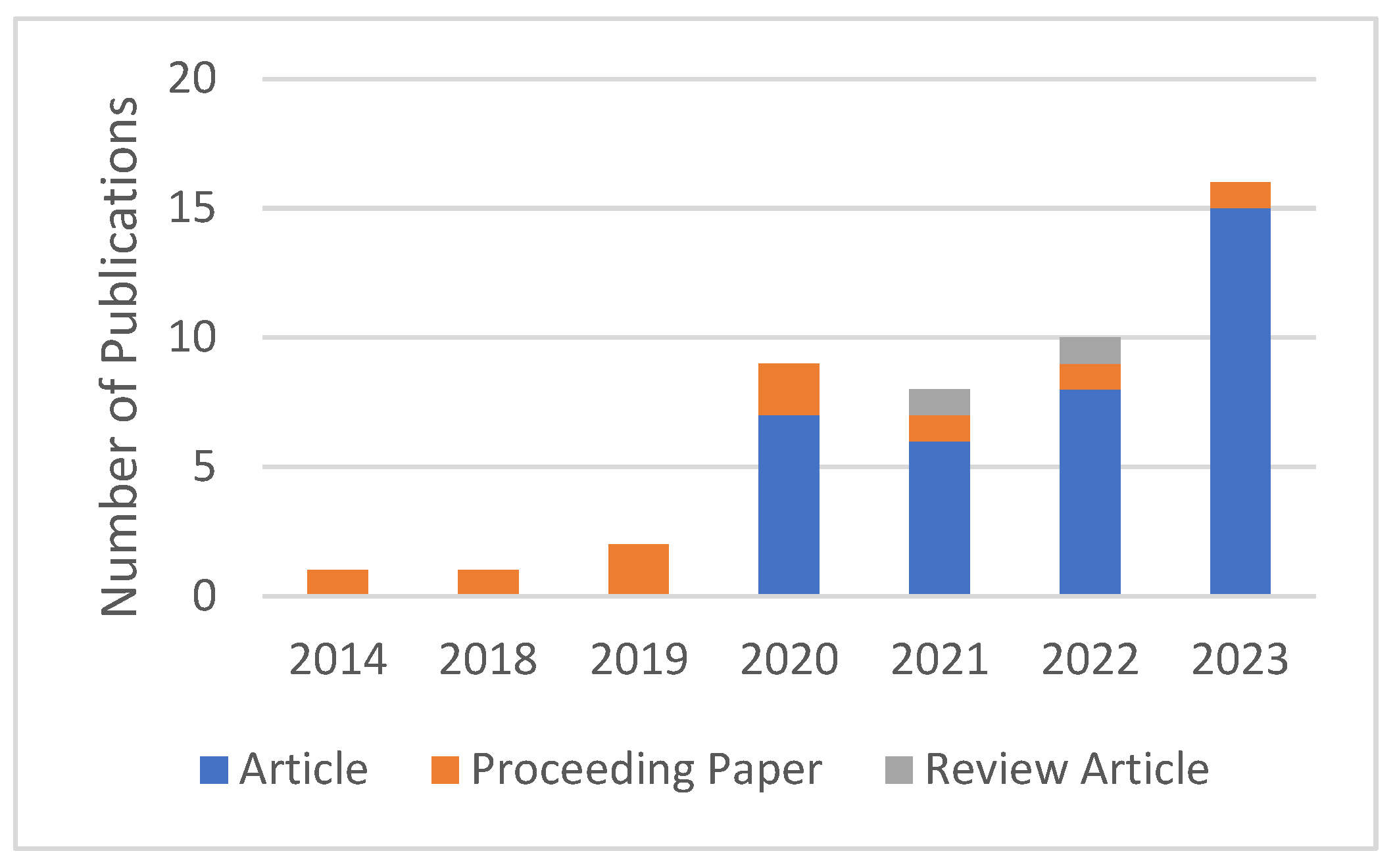
To solve the EVRP, the reinforcement learning method, one of the learning-based methods, stands out. EVRP studies that use reinforcement learning as a solution method are given in
Figure 2. To obtain
Figure 2, the WOS database was searched with the query “ALL = “electric vehicle” AND ALL = “reinforcement learning” AND (ALL = route planning OR ALL = path planning OR ALL = task scheduling OR ALL = routing)”. This query targeted papers that contained both the phrases “electric vehicle” and “reinforcement learning” and contained at least one of the phrases “route planning”, “path planning”, “task scheduling”, or “routing”.
Among these studies, Nazari et al. [
24] improve the pointer network by simplifying the recurrent neural network (RNN)-based encoder, which provides more efficient solutions to the VRP. Kool [
25] introduces a transformer-based architecture for the VRP, where both the encoder and the decoder part of the neural network use the attention mechanism. In this way, calculation speed and solution quality have increased significantly. In Soni et al.’s work [
26], the application of reinforcement learning techniques in electric vehicle (EV) movement planning is explored. The study focuses on optimizing battery consumption and evaluating EV travel time under various reinforcement learning schemes. A traffic simulation network is constructed using Simulation for Urban Mobility (SUMO) software, and both model-based and model-independent methods are applied. The findings reveal that Value Iteration proves to be an efficient algorithm in terms of battery consumption, average travel speed, vehicle travel time, and computational complexity. Q-learning is less successful in terms of travel time, despite demonstrating optimized battery consumption. Li et al. [
27] in their study use a new neural network integrated with a heterogeneous attention mechanism to strengthen the deep reinforcement learning policy to select nodes automatically. This way, solutions are produced by considering the priority relationships between nodes. Nolte et al. [
28] introduce Appointment Delivery, which aims to increase the efficiency of last-mile package delivery by taking advantage of the potential of Electric Autonomous Vehicles, especially in regions with high urbanization, such as Smart Cities. Additionally, for the optimization problem of finding the optimal delivery route for a particular delivery round, they propose two heuristic solutions based on state-of-the-art machine learning methods (attention mechanism, RNN) and reinforcement learning (actor–critic training). RL is a great advantage, especially for the problem under consideration, since optimal computational solutions for TSPs are computationally expensive or even infeasible. Lin et al. [
2] propose a novel method that employs deep reinforcement learning to address the EVRPTW. This advanced framework seeks to enhance routing decisions for electric vehicles (EVs) by incorporating considerations such as depot locations, battery levels, and visits to charging stations. Qi et al. [
3] propose a new RL-based algorithm for the energy management strategy of hybrid electric vehicles. A hierarchical structure is used in deep Q-learning algorithms (DQL-H) to obtain the optimal solution for energy management. This new RL method solves the sparse reward problem in the training process and provides optimal power distribution. DQL-H trains each level independently. Additionally, as a hierarchical algorithm, DQL-H can change how the vehicle environment is explored and make it more effective. Experimental results show that the proposed DQL-H method provides better training efficiency and lower fuel consumption than RL-based methods. Nouicer et al. [
4] propose a reinforcement learning approach with graph-based modeling to solve the Electric Vehicle Routing Problem with Time Windows. The aim of the article is to minimize the distance traveled while serving customers at certain time intervals by using the combination of Structure2vect and the Double Deep Q-Network. The proposed method is tested on real-world data from a public utility fleet company in Tunisia. The results reveal that the proposed model reduces the distance traveled by up to 50% and also optimizes the running time. Tang et al. [
5] extend the A2C approach by integrating a Graph Attention Mechanism (GAT) to address the EVRPTW. Their work also introduces an energy consumption model that accounts for factors such as electric vehicle mass, speed, acceleration, and road gradient. Wang et al. [
6] introduce a novel approach to the CEVRP by integrating deep reinforcement learning (DRL) with the Adaptive Large Neighborhood Search (ALNS). In this approach, operator selection is modeled as a Markov Decision Process (MDP), with DRL used for adaptive selection of destroy, repair, and charge operators. Rodríguez-Esparza et al. [
7] introduce the Hyper-heuristic Adaptive Simulated Annealing with Reinforcement Learning (HHASARL) algorithm to address the Capacitated Electric Vehicle Routing Problem (CEVRP). The algorithm integrates a reinforcement learning (RL) module as the selection mechanism and employs the Metropolis criterion from the well-established Simulated Annealing (SA) metaheuristic as its move acceptance component. Empirical results indicate that HHASARL demonstrates superior performance on the IEEE WCCI2020 competition benchmark.
3. Description of the ESOGU-CEVRPTW Dataset
A new dataset named ESOGU-CEVRPTW is generated for the Eskisehir Osmangazi University (ESOGU) Meselik Campus. The dataset has been uploaded to Mendeley Data [
34]. The ESOGU-CEVRPTW comprises 118 customers, ten charging stations, and a single depot. The dataset contains 45 different instances for the Capacitated Electric Vehicle Routing Problem with Time Windows. The CEVRPTW is a version of the CVRPTW, one of the VRP variants. The proposed dataset also includes information about EVs and charging stations. The dataset consists of test problem groups of five different sizes, with 5, 10, 20, 40, or 60 customers. Each test problem group contains instances from the random (R), clustered (C), and random–clustered (RC) customer distribution. Each group includes three different types of time windows: wide, medium, and narrow. All instances in the dataset are txt files. The dataset contains large-sized instances to test learning-based methods but also includes small-sized instances so that the problem can be solved by exact methods.
Dataset Generation
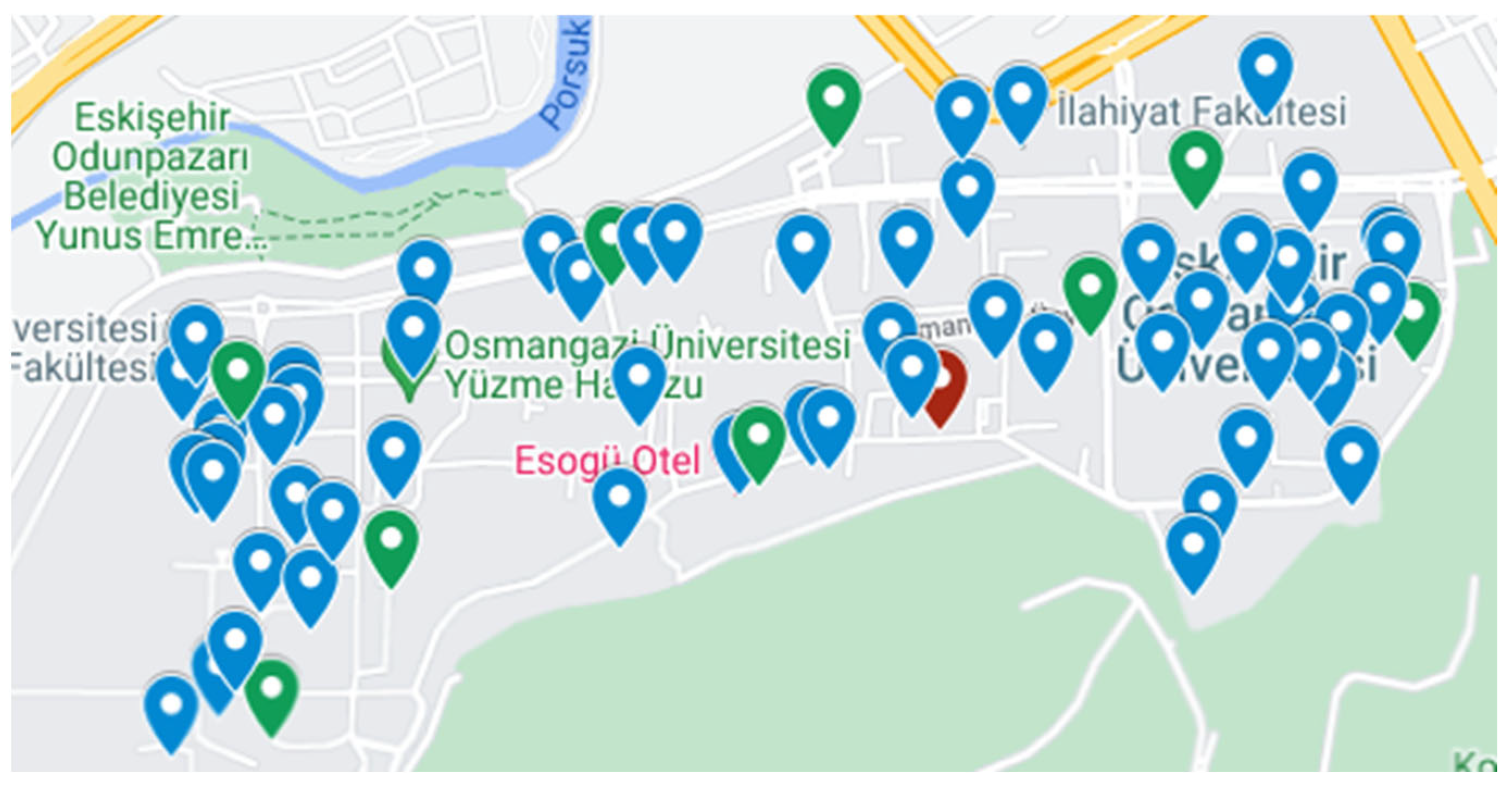
This section provides a detailed explanation of the dataset generation process. The generated dataset comprises real-world data, in contrast to those commonly found in the literature. The locations of the depot, customers, and charging stations within the dataset are based on geographical locations at the Eskisehir Osmangazi University Meselik Campus (
Figure 3). The map in
Figure 3 is generated using Google Maps, with geographical markers in different colors added to the specified points. In
Figure 3, the blue markers represent the delivery customers, and the green markers represent the charging stations.
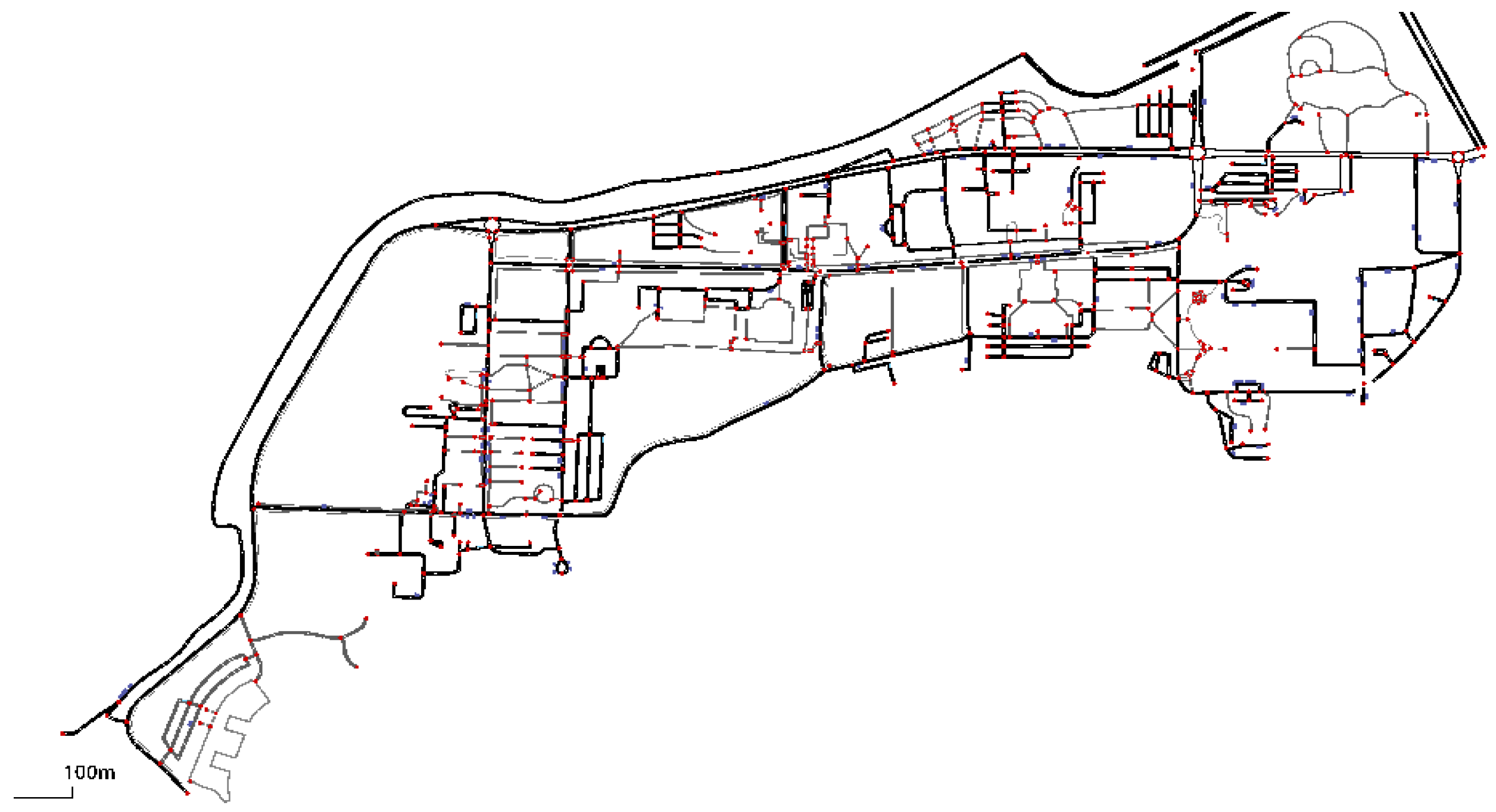
When generating the dataset, the road network of the ESOGU campus is transferred to the SUMO simulation environment. Information about all the buildings on the ESOGU campus is added to the SUMO. To display the buildings on the campus on the map, a container stop is added to the entry point of all buildings. The representation of the ESOGU campus in the SUMO Netedit environment is shown in
Figure 4. In
Figure 4, the blue container stop shows the pickup or delivery customers, and the green rectangles show the charging stations.
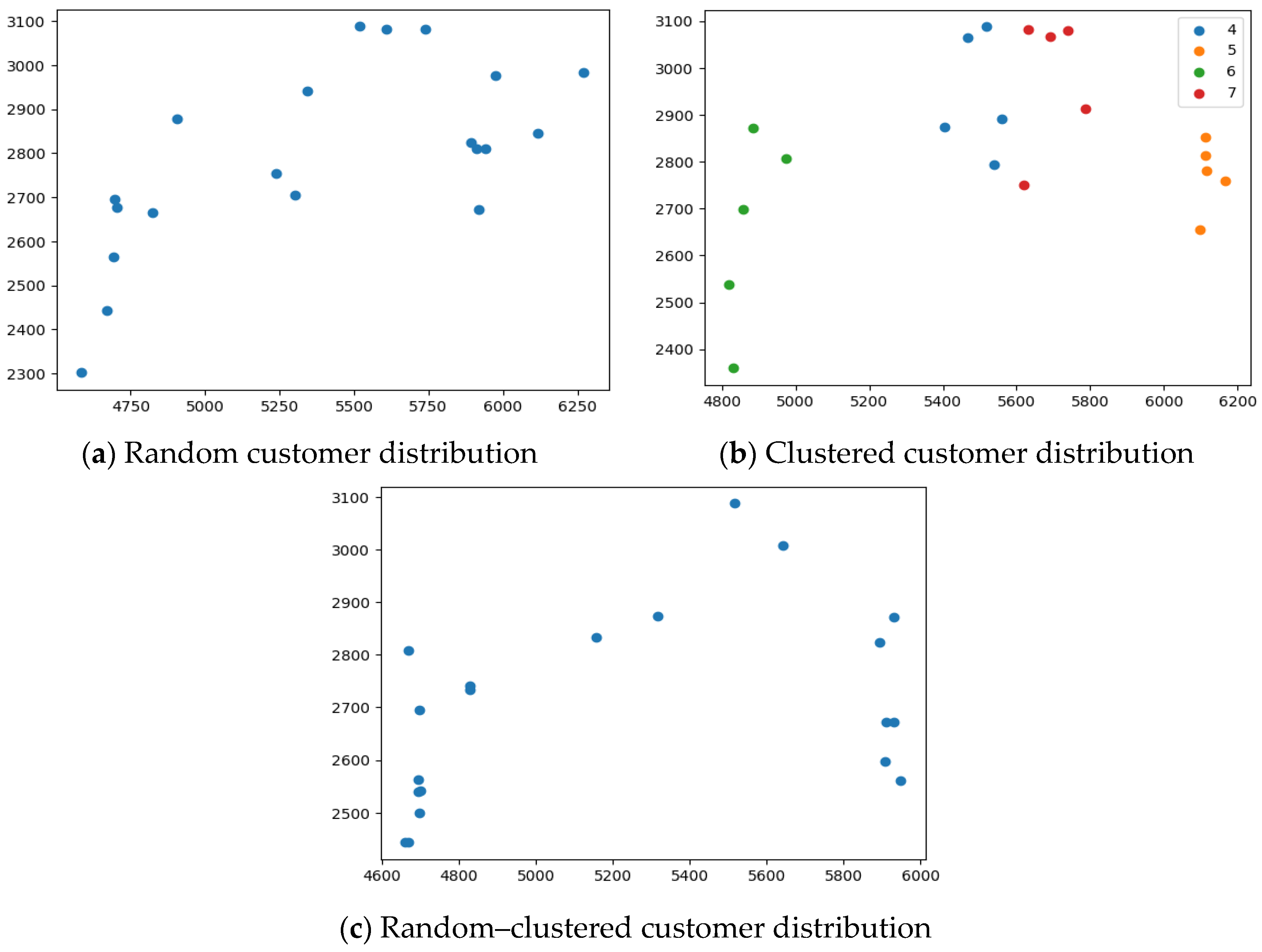
The dataset contains instances of different sizes, including 5, 10, 20, 40, and 60 customers. The customers have been selected in three different distributions, depending on the geographical distribution of the customer locations. These distributions are the random customer distribution (R), the clustered customer distribution (C), and the customer distribution (RC) which is a mixture of both.
Figure 5a illustrates the scenario where 20 customers are randomly selected from the 118 customers on campus for random customer distribution. Subsequently, 20 customers are selected from the customer clusters.
Figure 5b depicts the clustered distribution of these 20 customers. By merging both types of customer distributions, a random–clustered customer distribution is created, as shown in
Figure 5c.
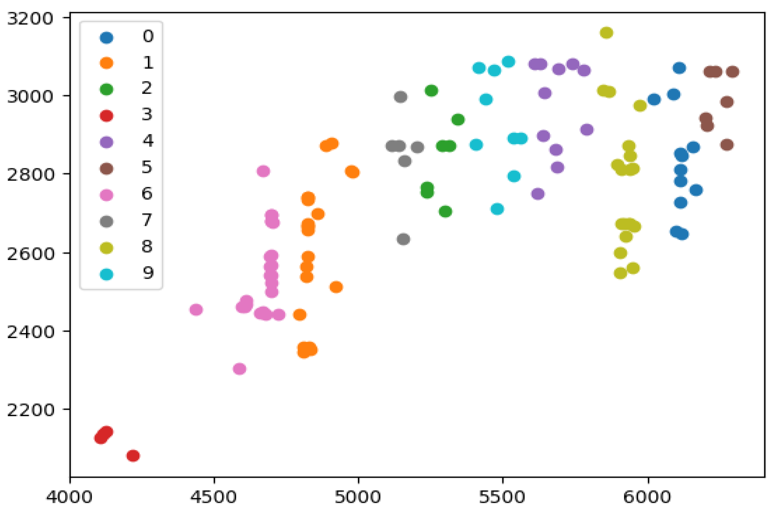
For the clustered customer distribution, the customers within the ESOGU campus have been divided into clusters using the K-Means algorithm.
Figure 6 illustrates the customers segmented into these clusters.
Following the identification of customers in the dataset, 10 parking spaces on the campus are designated as charging stations. The parameters in this dataset are generated to reflect real-world problems. To generate the time window constraint in the dataset, “the earliest start time to service” and “the latest start time to service” times for each customer are generated. The time window to start to service is generated by adapting the time window derivation mechanism from study [
35], originally used for the machine scheduling problem, to the Vehicle Routing Problem. The dataset includes three different time window horizons: narrow, medium, and wide. A narrow time window requires more vehicles to serve all customers compared to a wide time window.
Time windows, “the earliest start time to service” and “the latest start time to service”, are derived from a discrete uniform distribution using the formula presented in Equation (1).
refers to the travel time from the depot to the customer at normal speed,
denotes the duration of the pickup/delivery task for the customer (including walking times to and from the vehicle as well as pickup/delivery times), and
represents the number of vehicles. A wide time window, a medium time window, and a narrow time window are determined using the (
,
) values used in the study by [
35]. For example, a narrow time window is obtained by choosing (
,
) = (0, 1.2).
When the formula is applied for 118 customers and (α, β) = (0, 1.2), the time window is determined as [0, 1789]. This value [0, 1789] represents a narrow time window.
“Travel time” refers to the time it takes for the vehicle to traverse the distance between the depot and the customer. The Google Distance Matrix API is utilized to calculate this time. The Distance Matrix API can compute travel distance and duration for specific start and end points. Actual distance is used in these calculations instead of Euclidean distance.
“Service time” corresponds to the total time required for a person to deliver the goods to the customer via a pedestrian route after the vehicle reaches the nearest point to the customer, and for the person to return to the vehicle.
“Demand” for each customer in the problem is generated from a discrete uniform distribution between [19, 95].
The dataset includes a distance matrix that contains the shortest distances between all customers and charging stations on the ESOGU campus. The distance matrix is generated using SUMO. By utilizing these networks, the shortest path from one node (depot, customer, or charging station) to another node is calculated.
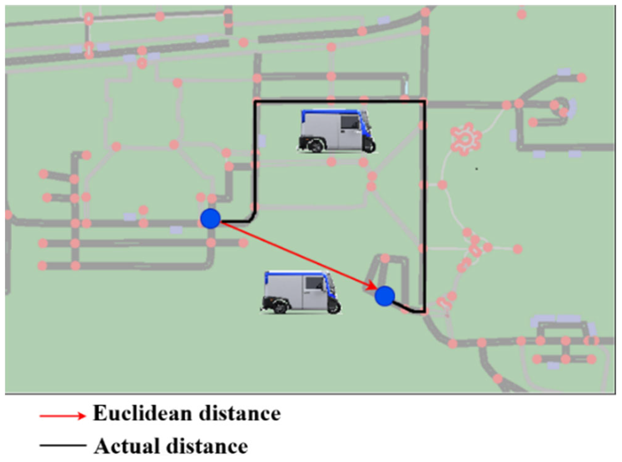
Figure 7 presents a comparison between the shortest paths computed using actual distances and Euclidean distances. As Euclidean distance does not accurately represent true travel distances, it fails to capture the complexities of real-world scenarios. The proposed dataset addresses this need by incorporating features such as buildings, streets, and other relevant infrastructure, thereby enabling route planning in a realistic environment with multiple attributes. This dataset, designed for real-world conditions, facilitates the application of advanced logistics methods. It provides a valuable resource for researchers, particularly those employing approaches that rely on environmental information, such as road characteristics (e.g., one-way, two-way, inclined, narrow), traffic regulations, and other factors. Moreover, the dataset offers the capability to simulate scenarios, such as road closures due to traffic accidents, allowing for the modeling of such situations in deep learning models.
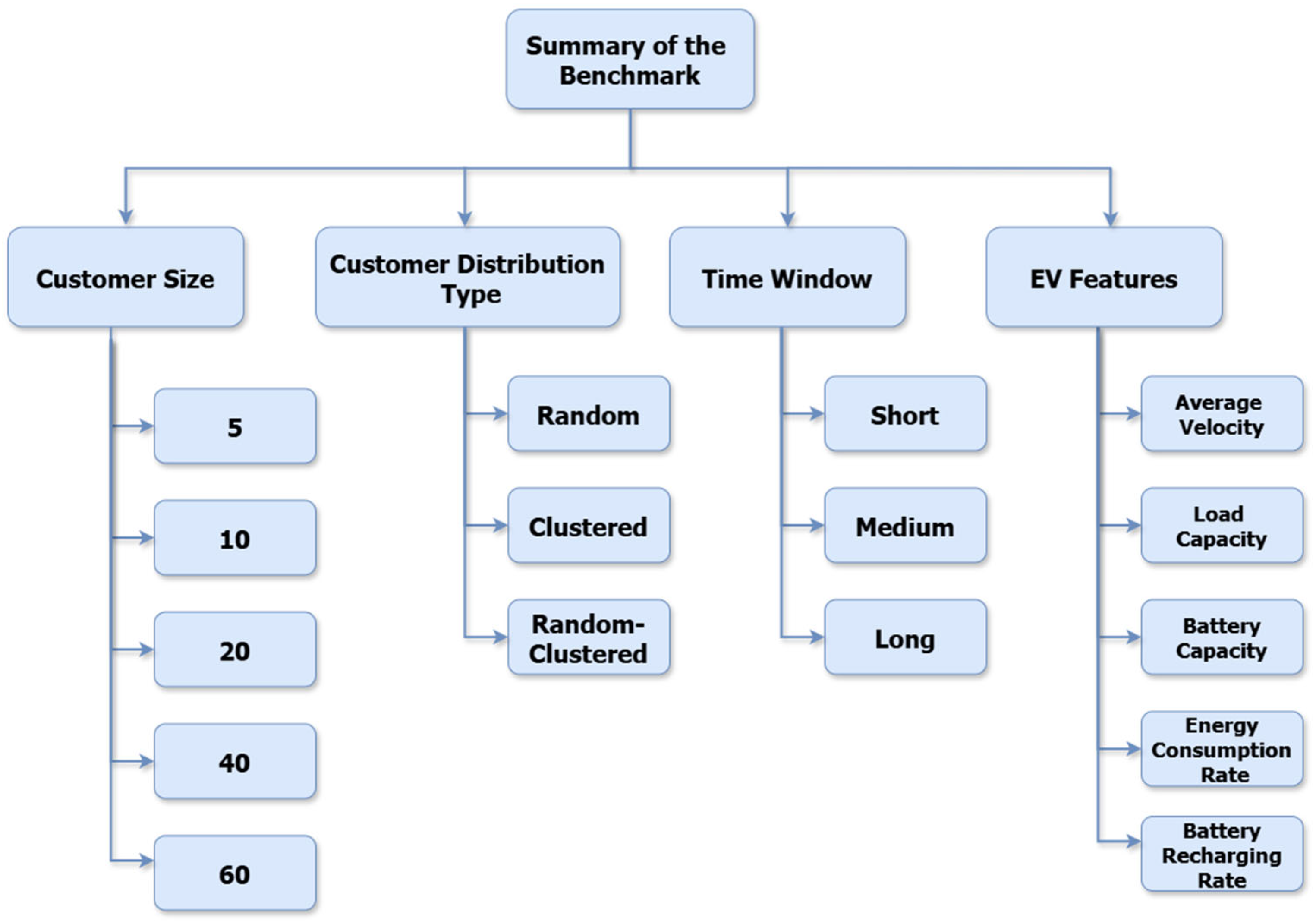
Figure 8 provides a description of the instances in the ESOGU-CEVRPTW dataset. It includes information on the number of customers in each instance, the distribution of the customers, and the time window applied. The generated dataset consists of real data from the ESOGU campus, with the campus map modeled in the SUMO simulation environment. An example problem from the dataset is presented in
Table 2.
Each location in the instance has an identifier (id), latitude and longitude, earliest start time to service, latest start time to service, demand and service time.
In the dataset presented within the paper, both the time window (TW) and without time window versions of the CEVRP are solved using a mathematical model to obtain optimal solutions. One of the objectives of developing a dataset based on real-world data is to fulfill the need for an ’environment’ for researchers working on EVRP using reinforcement learning. In line with this, the paper introduces the novel Q-learning method as a reinforcement learning approach to explore how the proposed dataset performs within the context of reinforcement learning.
4. Mathematical Model for the CEVRPTW
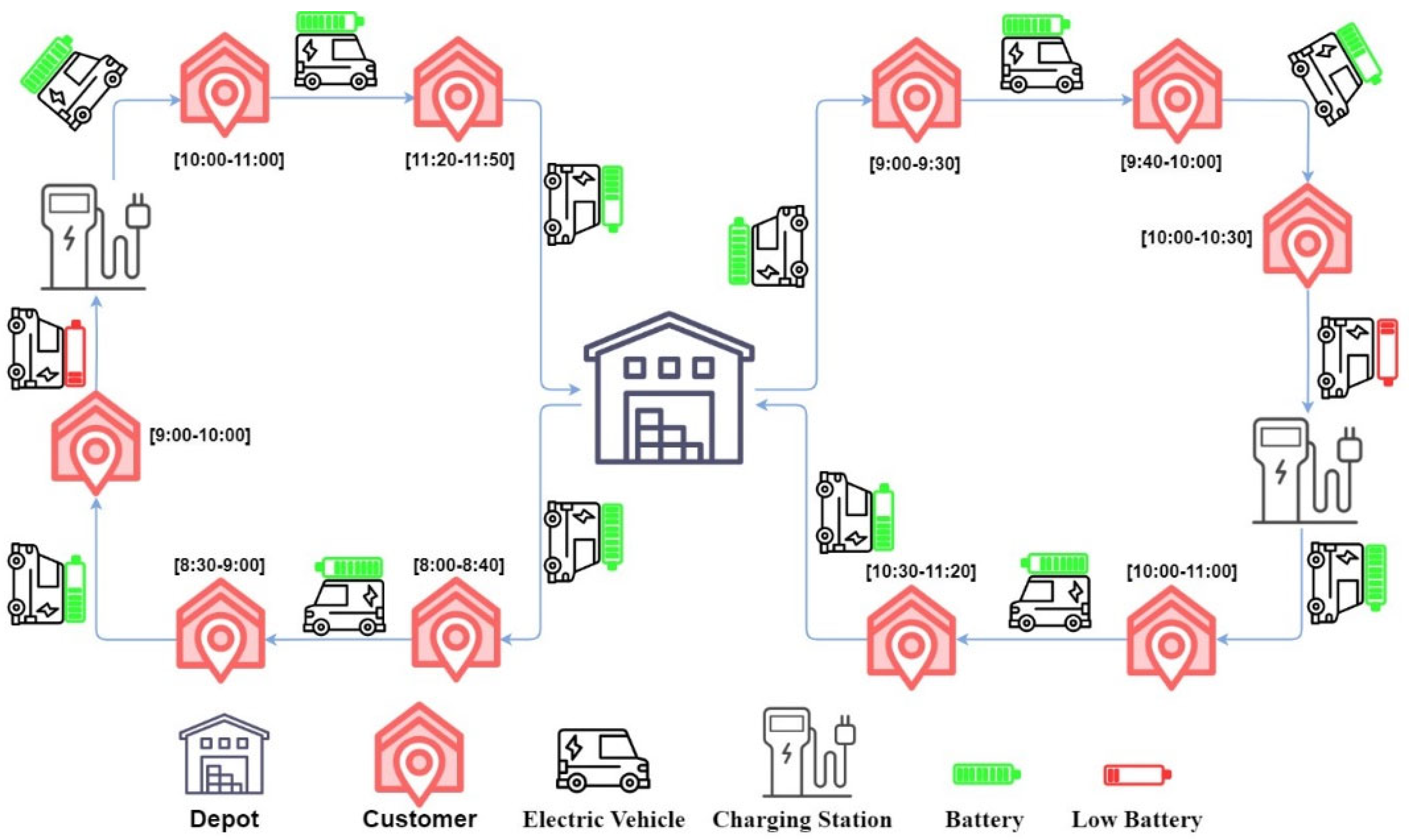
In this paper, the Capacitated Electric Vehicle Routing Problem with Time Windows is considered. The CEVRPTW is a combinatorial optimization problem. In the problem, EVs with a given payload and battery capacity leave from the depot fully charged. They leave from the depot to serve customers and visit stations to recharge their batteries throughout their routes. When an EV visits a charging station, it will be fully charged to complete its task. At the end of route, they must return to the depot. For EVs, the aim is to find routes where all customer demands will be met, and the fleet’s total distance or time traveled will be minimized. The CEVRPTW is initially defined as a complete directed graph
G = (
V,
E), as illustrated in
Figure 9.
V = {0 ∪
C ∪
F} represents the set of nodes in the graph. The depot is denoted by
0,
C represents the customers, and
F represents the charging stations.
E = {(
i,
j)|
i,
j ∈
V,
i ≠
j} is the set of edges. Each edge between nodes
i and
j has a distance value, denoted as
dij. [
ei,,
li] represents the time window of customer
i. When an electric vehicle travels on an edge, it consumes an amount of energy
ei,j =
h(
r)
·dij. h denotes the energy consumption rate.
This problem aims to minimize the total travel distance of all electric vehicles while serving customers within their time windows. There is a constraint that each customer can only be served one vehicle. EVs must return to the depot after fulfilling all customers’ demands. It assumes that electric vehicles are always fully charged at charging stations.
In the literature, Schneider et al. [
36] propose a mathematical model for the Capacitated Electric Vehicle Routing Problem with Time Windows. The model uses the following notation.
- 1.
Sets
| 0, N + 1 | Depot instances |
| F′ | Set of visits to recharging stations, dummy vertices of set of recharging stations F |
| F0′ | Set of recharging visits including depot instance 0 |
| V | Set of customers V = {1, …, N} |
| V0 | Set of customers including depot instance 0 |
| V′ | Set of customer vertices including visits to recharging stations V′ = V ∪ F′ |
| V0′ | Set of customers and recharging visits including depot instance 0: V0′ = V′ ∪ {0} |
| V′N+1 | Set of customers and recharging visits including depot instance N + 1: VN+1′ = V′ ∪ {N + 1} |
| V’0,N+1 | Set of customers and recharging visits including 0 and N + 1: V’0,N+1 = V′ ∪ {0} ∪ {N + 1} |
- 2.
Parameters
| qi | Demand of vertex i, 0 if i ∉ V |
| dij | Distance between vertices i and j |
| tij | Travel time between vertices i and j |
| ei | Earliest start of service at vertex i |
| li | Latest start of service at vertex i |
| si | Service time at vertex i (s0, sN+1 = 0) |
| C | Vehicle capacity |
| g | Recharging rate |
| h | Charge consumption rate |
- 3.
Decision Variables
| Pi | Decision variable specifying the time of arrival at vertex i |
| ui | Decision variable specifying the remaining battery capacity on arrival at vertex i |
| yi | Decision variable specifying the remaining battery capacity on arrival at vertex i |
| xij | Binary decision variable indicating if arc (i,j) is traveled |
- 4.
Mathematical Model
The mathematical model of the CEVRPTW is formulated as Mixed-Integer Linear Programming as follows [
36]:
The objective function (2) is to minimize the total travel distance. Constraint (3) ensures that service is provided to every customer node, constraint (4) ensures that the charging station can be visited, and constraint (5) prevents the formation of sub-tours. Constraints (6) and (7) guarantee time feasibility. Constraint (8) refers to the time window conditions. (9) and (10) are the constraints that control the vehicle’s load. Here, the vehicle will leave the depot with the load as much as its capacity. Constraints (11) and (12) control the vehicle’s charging status. Constraint (13) determines the number of routes. It gives the number of routes that will leave the initial warehouse and go to the nodes.
5. Reinforcement Learning for the CEVRP
Reinforcement learning (RL) involves an agent interacting with its environment to learn an optimal policy through trial and error for sequential decision-making problems across various fields. An RL agent engages with an environment over a period. At each time step
, the agent receives a state
from a state space
and chooses an action
from an action space
. The agent receives a reward
and transitions to the next
. The environment provides a reward to the agent based on the effectiveness of its actions. The agent experiments with various actions by assessing the total rewards received. Through numerous trials, the algorithm learns which actions yield higher rewards and develop a behavioral pattern. Over time, the agent aims to maximize the cumulative reward [
37].
RL algorithms are based on the Markov Decision Process (MDP). In this study, the route generation process to solve the CEVRP is considered a sequential decision-making problem. This problem is formulated using reinforcement learning (RL) and addressed accordingly. The route generation process is modeled as a Markov Decision Process (MDP). The elements of MDP are defined as state, action, transition rule, and reward function. In the study, states are nodes (depot, customers, charging stations), and actions are moving from one node to another node. RL aims to capture essential features of the environment with which an agent interacts to achieve its goal. The agent should be able to perceive the state of the environment and take actions that affect the state. RL aims to capture complex structures and go further than traditional machine learning by using more adaptable algorithms. RL algorithms have more dynamic behavior than conventional machine learning algorithms.
RL algorithms can be divided into two groups: model-based and model-independent. Model-based algorithms enhance learning by using precise knowledge of the environment. On the other hand, model-free algorithms can be applied without knowledge of the environment and can theoretically be adapted to any problem. These algorithms model the environment with MDP and learn strategies through interaction. Model-free algorithms can be divided into value-based, policy-based, and actor–critic. In this study, the Q-learning algorithm, one of the value-based algorithms, was used.
Proposed Q-Learning Algorithm
The Q-learning algorithm is a method of learning by interacting with the environment. It aims to learn strategies that tell agents what actions to take under what conditions. It does not need an environment model and can handle random transformation and reward problems. Q-learning finds the optimal strategy for any finite Markov Decision Process (FMDP). In this sense, it maximizes the total return expectation in all successive steps, starting from the current situation. Given the infinite search time and partially random strategy, Q-learning can determine the optimal action selection strategy for any FMDP.
This algorithm is an algorithm that uses a temporal difference algorithm and action-value-based off-policy. The action with the highest value among the possible actions is selected at each step. In other words, a greedy approach is applied. In this algorithm, a table called Q-table is created using situation–action pairs. The table size is the “number_of_states
number_of_actions”. To decide which action to choose from the current situation, the Q values in the table are looked at and the maximum Q value is selected. This algorithm works in discrete action sets and deterministic environments. The update rule that forms the basis of Q-learning is given in Equation (14).
(state, action) in Equation (14) is the current state, α is the learning coefficient, is the reward value in the reward table, γ is the discount factor, and represents the highest Q value of the places that can be visited.
In Q-learning algorithm, a RL agent engages with an environment over a period. At each time step , the agent receives a state from a state space and chooses an action from an action space . In our approach, the state representation consists of current node id, current battery capacity, and current cargo capacity information. Action determines the node that the EV goes to at step . The sequence of actions is generated from the initial step 0 to the final step T. Here, is the action of departing from the depot, is the action selected at the first step, and is the action of returning to the depot. The action space represents a set of discrete actions. The agent decides to go to a customer, a charging station, or a depot.
An essential aspect of the Q-learning algorithm is the balance between exploration and exploitation. Initially, the agent lacks knowledge about the environment and is more inclined to explore rather than utilize existing knowledge. Over time, as the agent interacts with the environment, it gains understanding and increasingly relies on this acquired knowledge. It is crucial to strike a balance between leveraging this knowledge and continuing to explore new possibilities. Without this balance, the Q-value function may converge to a local minimum rather than the optimal solution. To address this, the exponential decay formula is employed.
In the study, several enhancements have been implemented to the state-of-the-art version of Q-learning, as outlined in studies in the literature [
12], to better address the CEVRP problem. One of the key modifications is the use of a masking technique, which generates possible actions by masking the nodes that the electric vehicle (EV) cannot reach. This ensures that the EV selects from only the feasible actions at each step. By filtering out infeasible options, the masking mechanism enhances the agent’s focus on valid actions, thereby aiding in the construction of feasible solutions. The masking function generates a list of feasible actions based on the current state, considering factors like battery level, vehicle capacity, time windows, and visited customers. Invalid actions, such as moving to a node that cannot be reached due to insufficient battery or capacity, are masked out.
If customer node i has already been visited, it is masked.
If node i represents a customer, its unsatisfied demand exceeds the remaining cargo capacity of the EV, and node i is masked.
If the EV is currently at customer i and its battery level is insufficient to visit the next customer j and return to the depot or any charging stations, customer j is masked.
If the EV is currently at any node i and its battery level is insufficient to visit the next charging station j and return to the depot or any charging stations, charging station j is masked.
If a self-loop is detected, where the agent would revisit charging stations or depots unnecessarily before completing new deliveries, the corresponding action is masked to encourage more efficient routing.
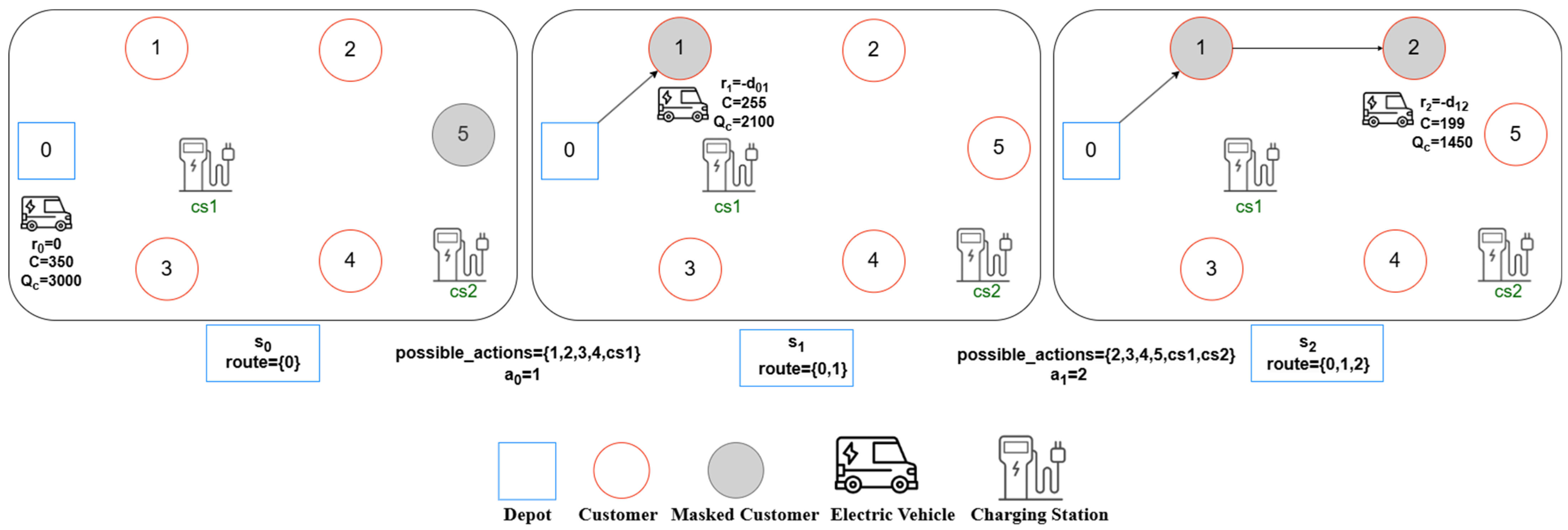
Additionally, in contrast to the classical Q-learning approach, where the epsilon-greedy strategy relies on a fixed epsilon value to balance exploration and exploitation, we have adopted an Epsilon Decay Strategy. This dynamic adjustment of epsilon ensures a more adaptive exploration–exploitation trade-off, which can be more effective than a static epsilon throughout the learning process. These updates aim to improve the performance and applicability of Q-learning in solving the CEVRP. The step-by-step representation of the proposed Q-learning algorithm is shown in
Figure 10. In the initial step of the algorithm, the depot is designated as
and added to the route list. Accessible actions from this initial state are determined through masking and included in the
feasible_actions list. Specifically, customer 5 is masked in this step, as it is unreachable from
with a battery capacity of 3000.
The pseudo-code of the proposed Q-learning algorithm to solve the CEVRP is presented in Algorithm 1 and Algorithm 2. First, the algorithm creates a Q table with the “states_size × action_size”. The created Q table is initially filled with zeros because the agent has no experience. The training process begins with the initialization of the neural network weights. Subsequently, entire iteration is executed until the agent reaches a terminal state, which is determined by the completion of the tour with all customers served. At each new state st, the agent selects an action using an epsilon-greedy policy balancing exploration and exploitation. Early in training, it is more likely to choose actions randomly (exploration). Over time, as it becomes smarter, the epsilon value decreases, meaning the agent increasingly exploits the knowledge it has gained so far by picking the best action based on the Q-values predicted by the model. When the agent wants to explore (i.e., the random number is below epsilon), it selects a random action from the set of feasible actions determined by the masking scheme. Otherwise, it computes the Q values for the current state and feasible actions, then selects the action that achieves the highest Q value. The chosen action updates the EV’s route, battery level, and capacity based on the selected node (e.g., moving to a customer, charging station, or depot). The reward for the action is calculated using the reward function in Equations (15) and (16), which penalizes the agent for longer distances while incentivizing efficient route planning. After the agent executes an action, the environment transitions to a new state, reflecting the updated EV’s status (battery, capacity), location, and current node information.
| Algorithm 1: Proposed Q-learning algorithm |
1: Initialize Q table with zeros and large negative number for self-loops.
2: Set maximum number of iterations .
3: Set .
4: Set initial epsilon , minimum epsilon ,
5: Initialize .
6: while
7: Initialize visited customers list.
8: Initialize route_list to empty list.
9: Initialize .
10: Initialize
11: Initialize and .
12: while True do
13: if all customers visited and current state is the depot then
14: complete_route = True.
15: end if
16: Generate a list of feasible_actions according to the masking scheme
17: if feasible_actions is empty then
18: complete_route = False
19: end if
20: Select action from feasible_actions using epsilon-greedy policy
21: Execute step function with selected action and get reward and next state
22: Update Q value using Bellman’s equation.
23:
24:
25:
26: Update epsilon
27: end while
28: if complete_route = True then
29: add route and its total distance route_list.
30: end if
31: Increment .
32: end while |
| Algorithm 2: Step Function |
input: state, action, current_load_capacity, current_battery_capacity)
output: reward, state, current_load_capacity, current_battery_capacity
1: Initialize charge_consumption rate =1.
2:
3: if can go to this action based on the charge consumption and customer demand then
4: state=customer
5:
6: update current_load_capacity, current_battery_capacity.
7: end if
8: else if cannot go to this action based on the charge consumption
9: choose the random charging station
10: state =charging station
11:
12: update current_battery_capacity.
13: end if
14: else if cannot go to this action based on the customer demand
15: state =depot
16:
17: update current_load_capacity, current_battery_capacity.
18: end if
19: Return reward, state, current_load_capacity, current_battery_capacity |
The episode terminates when the agent successfully visits all customers and returns to a depot. If the agent runs out of battery or fails to complete the route, the episode ends, and the agent learns from the failure. Successfully completed routes are recorded, and the agent strives to minimize the total distance traveled while satisfying customer demand. The algorithm starts with a predefined maximum number of iterations. At every 100th iteration, the route with the lowest cost is identified from the list of completed routes. Subsequently, the algorithm evaluates whether the most recently identified lowest cost route is identical to the previously determined lowest cost route. If the lowest cost route remains unchanged for a consecutive series of iterations (specifically, 2000 iterations), the algorithm is considered to have achieved convergence, thereby terminating the iterative process.
6. Experimental Results
In this section, experiments are conducted on the ESOGU-CEVRPTW dataset to evaluate the performance of the proposed mathematical model in solving the CEVRPTW. Additionally, the proposed Q-learning algorithm for solving the CEVRP is tested on the ESOGU-CEVRPTW dataset and compared with the optimal results.
6.1. Results of the Mathematical Model
The proposed mathematical model is used to obtain optimal routes on the presented dataset. Optimal results are obtained with the CPLEX solver for the generated ESOGU dataset.
Table 3 shows the mathematical model results for CEVRP without including the time window constraint for some instances in the dataset. The execution time, the minimum distance, the number of routes, and the optimal route for solved instances are shown in
Table 3. The mathematical model can produce results in a reasonable time for small-sized problems involving 5, 10 customers. For the solution of large-sized problems involving 20, 40, and 60 customers, the model is run for approximately 3 h and results are given in
Table 3. Optimal results could not be obtained in a reasonable time for large-sized problems.
Video in reference [
38] shows the optimal route obtained by the mathematical model, for ESOGU_C10 instance in the dataset. The obtained optimal routes are visualized in SUMO. The routes for the ESOGU_C10 are as follows: R1: D-45-22A-CS8-14-D R2: D-CS4-26-113-CS6-24-13-D R3: D-119-34-31-D. In video the route shown in yellow represents R1, the route shown in red represents R2, and the route shown in blue represents R3.
Mathematical models provide an exact formulation of routing problems, such as the Electric Vehicle Routing Problem (EVRP), by explicitly defining constraints and objective functions. In contrast, Q-learning transforms the same problem into a reinforcement learning framework, representing it through actions, states, and rewards. While mathematical models aim to find an exact solution to the problem, the Q-learning algorithm approaches the objective function value by conducting a learning process based on rewards and penalties. In mathematical models, constraints are explicitly defined, and the solution is required to strictly adhere to them. However, in Q-learning, these constraints are indirectly learned through the reward function. While mathematical models yield exact solutions, Q-learning, as a learning-based approach, produces solutions that improve and converge over time. This feature is particularly advantageous for solving large-scale and complex problems where exact methods may become computationally prohibitive.
6.2. Results of Proposed Q-Learning Algorithm
In the study, the proposed Q-learning model for the CEVRP is tested on the presented ESOGU-CEVRPTW dataset. As the problem addressed does not include a time window constraint, this constraint is disregarded in the dataset. The vehicle’s load capacity is 350 kg, and the battery capacity is 3000 kWsec. A relatively small battery capacity is utilized to ensure that the constraints related to visiting charging stations are effectively demonstrated in the test environment.
The proposed method is tested on 15 instances from the dataset. In each instance, the number of routes varies based on the number of customers and their demands. The EV starts from the depot and satisfies the customers’ demands as long as its load capacity permits. When the current load capacity is insufficient, the EV returns to the depot to reload to full capacity. Additionally, if the EV’s charge level is insufficient to reach the next customer while on the route, it is directed to the most suitable charging station for a full recharge. The aim is to calculate the shortest distance route by complying with the constraints of customer demand and the state of charge of the EV.
All the tests are performed on a desktop with i5-7500 CPU (3.40 GHZ and 12 RAM). The code is written in Python 3.8. To evaluate the performance of the proposed model, the model is trained and tested on various sample sizes ranging from n = 5 to 10, 20, 40, or 60 client nodes. The training is performed using the hyperparameters summarized in
Table 4. The hyperparameters presented in
Table 4 are determined through mutation-based white-box testing, as described in [
39]. The study [
39] focuses on mutation-based tests of a reinforcement learning (RL) model developed for electric vehicle routing, a Long Short-Term Memory (LSTM) model, and a transformer-based neural network model. The deep mutation module is a tool developed to assess the robustness and accuracy of deep learning models. It can be utilized for various types of deep models, and since these models employ distinct structures, the evaluation metrics used vary depending on the model type. In RL models, metrics may vary depending on the model. Reward_max, a metric used to find the most optimal route for electric vehicles, is used in the RL model. The module classifies mutants as “killed” if these metrics decrease or “survived” if the opposite occurs. The parameters gamma, alpha, epsilon, and decay for the RL model were selected and for each parameter, 29, 40, 30, and 26 mutants were generated, respectively.
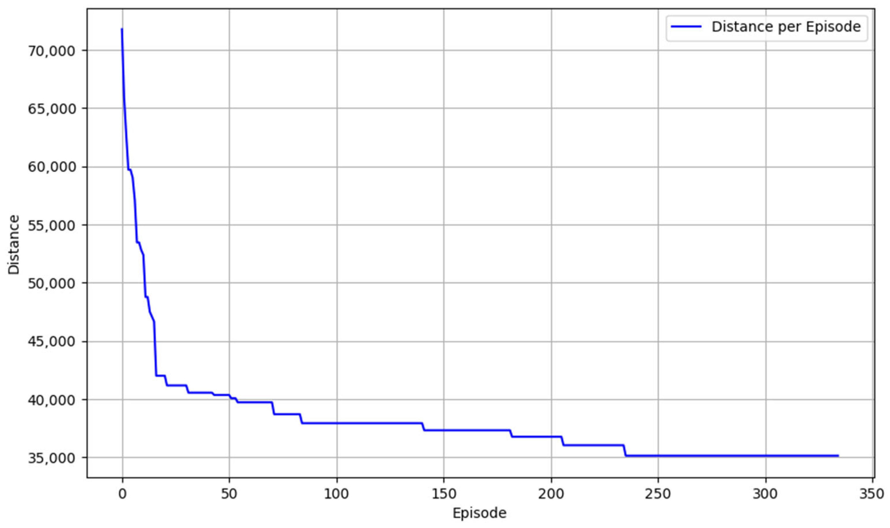
The learning curve presented in
Figure 11 depicts the performance of the Q-learning algorithm in minimizing the total distance traveled across multiple training episodes for the ESOGU_RC60 instance. Data points are sampled and plotted every 20 episodes to provide a comprehensive overview of the algorithm’s learning progression. Initially, the total distance may exhibit higher values, reflecting the agent’s exploratory behavior and suboptimal routing decisions. As training progresses, a general downward trend is observed, indicating that the Q-learning agent is effectively learning and refining its policy to achieve more efficient routes. This reduction in total distance over successive episodes demonstrates the algorithm’s capacity to optimize routing decisions, thereby enhancing overall performance. The stabilization of the curve toward lower distance values suggests that the algorithm is approaching convergence, consistently identifying near-optimal solutions for the CEVRP.
The proposed method was tested on the ESOGU_CEVRPTW dataset, and the vehicle capacity was accepted as 350 and the vehicle battery as 3000. The proposed method also works on different datasets, such as a sparser dataset or for EVs with different battery capacities. In addition, in order to show that the proposed method can work in situations that require multiple charging stops on a route, an additional experiment was designed to reduce the vehicle’s battery capacity and accept it as 1000. In this case, in order to proceed even between two customers, the vehicle had to stop at more than one charging station. When the EV battery capacity is 3000, the routes generated by the proposed algorithm are “R1: D-35-32-115-2-CS9-D R2: D-42B-D” and the total distance is 3989.19 m. When the battery capacity is 1000, the routes generated are “R1: D-32-CS8-115-2-CS9-CS7-35-D R2: D-42B-D” and the total distance is 4686.75 m. In this scenario, it is observed that the electric vehicle requires multiple charging stops between two customer locations.
In this study, the proposed algorithm is compared with the mathematical model and Double Deep Q-Network (DDQN) algorithm [
29]. The DDQN is a reinforcement learning algorithm and an enhancement of the conventional Deep Q-Network (DQN). The DDQN employs two distinct networks, namely the main network and the target network, to mitigate the overestimation bias that can arise during Q-value estimation. The DDQN model is one of the effective reinforcement methods that has been widely applied in many areas, especially in recent years, including routing problems (e.g., VRP, E-VRP, etc.). In the literature, recent studies using the DDQN model for the VRP and EVRP can be found in references [
4,
29,
40]. The DDQN model presented in [
29] was employed to solve the CEVRP problem and compared with the proposed method in our study.
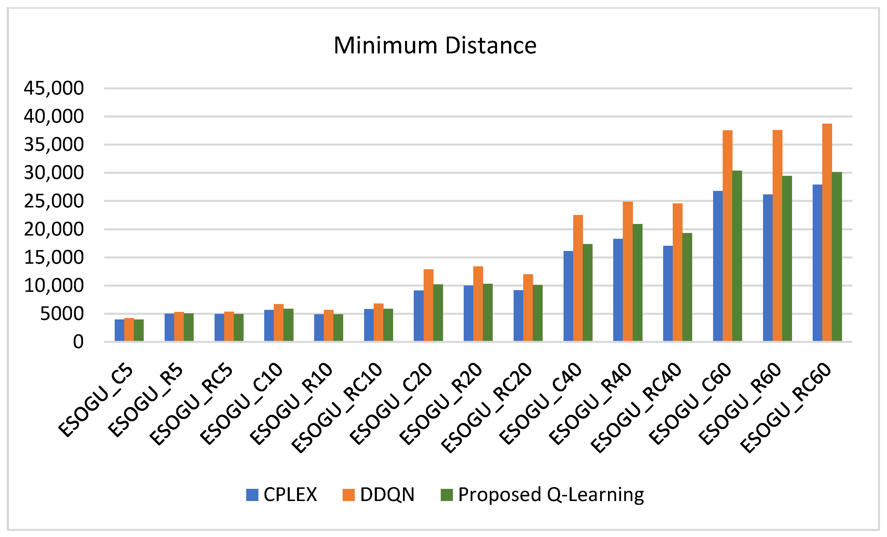
Table 5 shows the comparative results of the mathematical model, DDQN algorithm, and the proposed Q-learning algorithm.
The proposed Q-learning model gives results close to the optimal solutions in small test problems, as illustrated in
Figure 12. Furthermore, the proposed Q-learning algorithm outperforms the DDQN algorithm, yielding shorter total distances. This superior performance can be attributed to the Q-learning algorithm’s ability to effectively balance exploration and exploitation, thereby identifying more optimal routing paths.
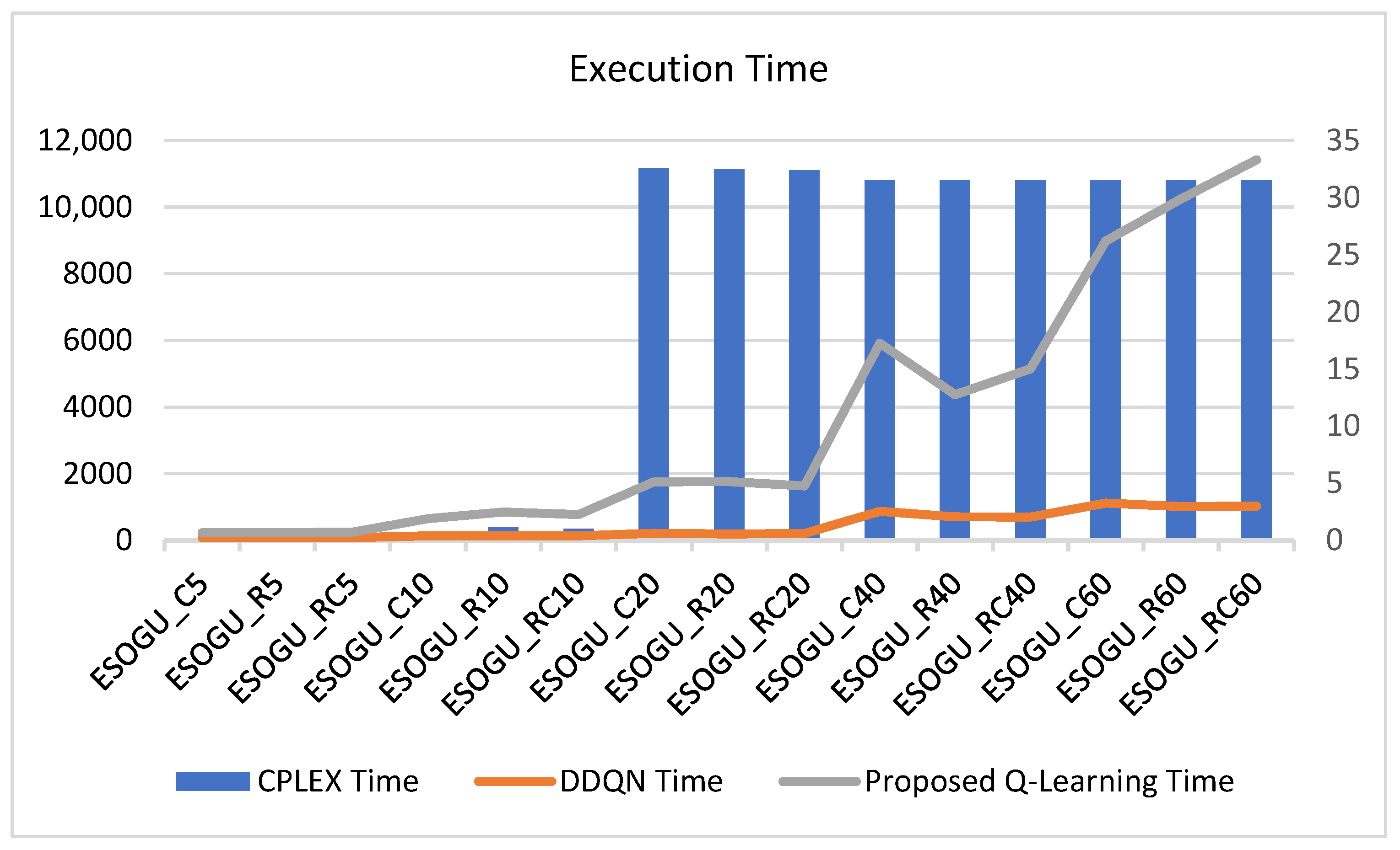
Compared to the mathematical model, the proposed Q-learning model significantly reduces the execution time. Large-scale problems can be solved in approximately 30 s, in contrast to the 3 h required by the mathematical model. Thus, the proposed method demonstrates markedly shorter execution times, as illustrated in
Figure 13. In terms of execution time, both the DDQN and Q-learning algorithms exhibit significantly faster computation times compared to the mathematical model. While the mathematical model, despite providing optimal solutions, requires considerable computational resources and time, the reinforcement learning approaches (Q-learning and DDQN) offer near-instantaneous solutions. This substantial reduction in computation time underscores the practical applicability of reinforcement learning methods in real-world logistics operations, where timely decision making is crucial.
Within the scope of last-mile delivery, algorithms capable of producing high-quality solutions in a short time are critical for companies. Overall, the comparative analysis highlights that the proposed Q-learning not only approximates optimal solutions with high accuracy but also surpasses the DDQN in distance efficiency while maintaining superior execution speed relative to traditional mathematical models. These attributes make Q-learning a highly promising approach for solving the CEVRP in operational settings, offering a balanced trade-off between solution quality and computational efficiency. This study demonstrates that Q-learning can achieve near-optimal solutions in a significantly reduced execution time.


