Article

Soil Parameter Inversion Considering the Influence of Temperature Effects

1
Beijing Uni.-Construction Group Co., Ltd., Beijing 100088, China
2
Department of Civil Engineering, University of Science and Technology Beijing, Beijing 100083, China
*
Author to whom correspondence should be addressed.
Appl. Sci. 2025, 15(23), 12511; https://doi.org/10.3390/app152312511
Submission received: 20 October 2025 / Revised: 13 November 2025 / Accepted: 17 November 2025 / Published: 25 November 2025

Abstract

Significant environmental temperature variations occur during the construction of large-scale underground structures, constituting one of the major factors influencing structural deformation. Parameter inversion of soil layers based solely on the causal relationship between excavation-induced loading effects and structural displacements can lead to substantial errors. To address this issue, this study aims to improve the inversion accuracy of soil parameters by considering temperature effects. A finite element model incorporating temperature effects, combined with machine learning algorithms, was employed to improve the inversion process. Based on the measured displacements and structural temperatures of diaphragm walls of the Beijing Tongzhou Integrated Transportation Hub Project, the influence of temperature effects on structural behavior was investigated to improve the inversion accuracy of soil parameters for large underground structures. Then, a finite element model of the excavation considering temperature effects is established using measured soil parameters and temperature data. According to soil classification, a training dataset is constructed through proportional scaling of soil parameters. Three machine learning algorithms—Decision Tree, Random Forest, and Gaussian Process Regression—are compared to evaluate inversion accuracy. The results indicate that the deformation of underground structures is governed by the coupled effects of temperature and earth pressure. Among the tested methods, the Random Forest algorithm demonstrates the highest accuracy in soil parameter inversion, with an average displacement error of 4.23% in the finite element model based on the inverted parameters. These findings highlight the importance of incorporating temperature effects to enhance inversion reliability for large underground structures.

1. Introduction

With the development of China’s modern integrated transportation system, the development and utilization of underground space have gradually become a major focus of infrastructure construction. During the construction of underground structures, monitoring indicators such as the displacement of retaining structures, ground uplift, and surface settlement are commonly used to evaluate the construction safety [1]. Although these indicators enable timely assessment of excavation-induced deformations, they are insufficient for predicting the future evolution of deformation. To investigate the deformation behavior of excavations, numerical methods have been widely applied. However, due to the irregularity of stratigraphic structures, the heterogeneity of soils, and the uncertainty of constitutive models [2], it is often necessary to employ inversion techniques to obtain the equivalent geotechnical parameters.
Conventional back-analysis of parameters primarily establishes regression models between influencing factors and response quantities based on statistical theory, including the least-squares method [3], the Levenberg–Marquardt algorithm [4], and nonparametric regression approaches [5]. With the advancement of machine learning theory, intelligent optimization and learning algorithms—such as genetic algorithms [6], particle swarm optimization (PSO) [7], and neural networks [8]—have also been introduced into soil parameter inversion. Cheng et al. [9] proposed a soil parameter inversion framework that couples PSO with multi-output least-squares support vector regression and identified the elastic modulus of soils for a foundation pit in Shenzhen. Ji et al. [10] employed a real-coded hybrid genetic algorithm to identify pressuremeter test parameters and excavation soil parameters. Cao et al. [11] developed a simulated annealing–particle swarm hybrid optimization scheme for least-squares support vector machines, demonstrating good applicability to foundation-pit inversion problems characterized by small samples and nonlinearity. Zhao et al. [12] combined a backpropagation neural network with multi-objective PSO for deep-excavation parameter identification and predicted the lateral displacement of support piles. Liu et al. [13] calibrated the Clay and Sand Model parameters using a Bayesian optimization–genetic algorithm strategy informed by stress–strain data. Li and Sima [14] optimized neural network weights via a mind evolutionary algorithm to invert excavation-induced horizontal displacements, thereby enhancing the practical utility of geotechnical parameter inversion. Liu et al. [15] leveraged a bidirectional long short-term memory network to extract temporal features from multi-period lateral displacements of diaphragm walls and mapped them to key parameters of the hardening soil small-strain (HSS) model, achieving close agreement between predicted and monitored wall displacements. Sun et al. [16] proposed an Elman neural network-based displacement prediction method optimized by the mind evolutionary algorithm and enhanced by variational mode decomposition, decomposing monitored displacements into trend, periodic, and stochastic components for rolling prediction.
Usually, geotechnical parameter inversion did not account for temperature effects. The construction of large underground projects requires a long time to complete; thus, the ambient temperatures vary significantly because of different seasons [17,18]. Consequently, the displacements recorded by structural monitoring points reflect the coupled influence of excavation-induced unloading and temperature actions. Ji and Shi [19] examined retaining-structure responses under both heating and cooling scenarios and concluded that cooling exerts a more pronounced impact on internal forces and displacements. Park et al. [20] conducted three-dimensional thermomechanical monitoring of diaphragm walls in deep excavations and systematically evaluated the effects of artificial ground freezing on wall displacements and internal forces. Lu et al. [21] coupled the temperature and stress fields to analyze temperature effects on braced retaining systems and recommended treating temperature as an explicit working condition in excavation design and analysis. Liu et al. [22] investigated seasonal temperature variations and their influence on support forces and deformations, further discussing how soil stiffness modulates thermally induced stresses. Wang et al. [23], through physical modeling and numerical simulation, explored the interaction between the evolving temperature field during freezing and diaphragm-wall behavior, and proposed a safety range for frost-heave pressure along the freezing interface.
When performing inversion of traditional soil layer parameters, it is assumed that the monitored structural horizontal displacements are induced solely by the excavation of soil mass, while the influences of temperature are neglected.
To achieve this objective, the study aims to (1) investigate the influence of temperature effects on the displacement behavior of underground structures through field monitoring and (2) establish a soil parameter inversion method for large excavations that explicitly accounts for temperature effects.
Based on the field monitoring data from the Beijing Tongzhou Integrated Transportation Hub, the displacements and temperatures of the diaphragm walls were measured at different structural levels. Soil parameters were determined through laboratory testing and soil classification. Proportional scaling of parameters was applied to generate finite element (FE) models, and temperature differences across construction stages were incorporated to assemble a training dataset reflecting temperature effects. Finally, the inversion accuracy of the three algorithms was comparatively evaluated. The flowchart of this study is shown in Figure 1.

2. Influence of Temperature on Underground Structural Deformation

2.1. Experimental Monitoring of Displacement and Temperature in Underground Structures

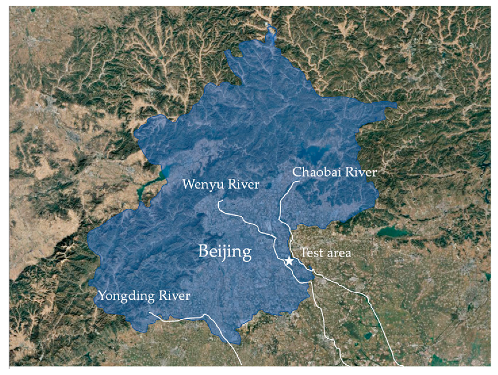
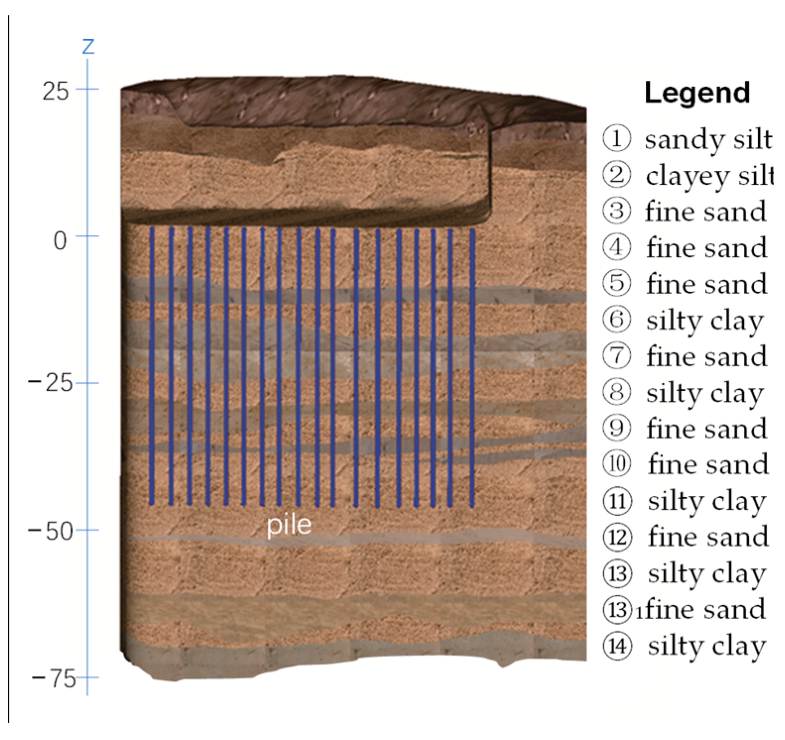
Beijing’s Tongzhou District is situated on an alluvial–proluvial plain formed by the Yongding, Chaobai, and Wenyu Rivers [24,25]. The location of Tongzhou and these three rivers are shown in Figure 2. The strata comprise artificial fill, younger sediments, and Quaternary deposits. The artificial fill consists of miscellaneous fill and construction-debris soils; the younger sediments are dominated by cohesive soils in an underconsolidated state. The Quaternary sequence features interbedded layers of clay, silt, and sand. The strata were mainly formed by alternating fluvial and lacustrine sedimentation, resulting in horizontally continuous but locally variable layers. Figure 3 shows the distribution of soil layers. The sand layers are relatively dense and permeable, whereas the clay and silt layers are soft and exhibit low permeability. This interbedding produces a heterogeneous soil profile that exerts a significant influence on deformation behavior during excavation.
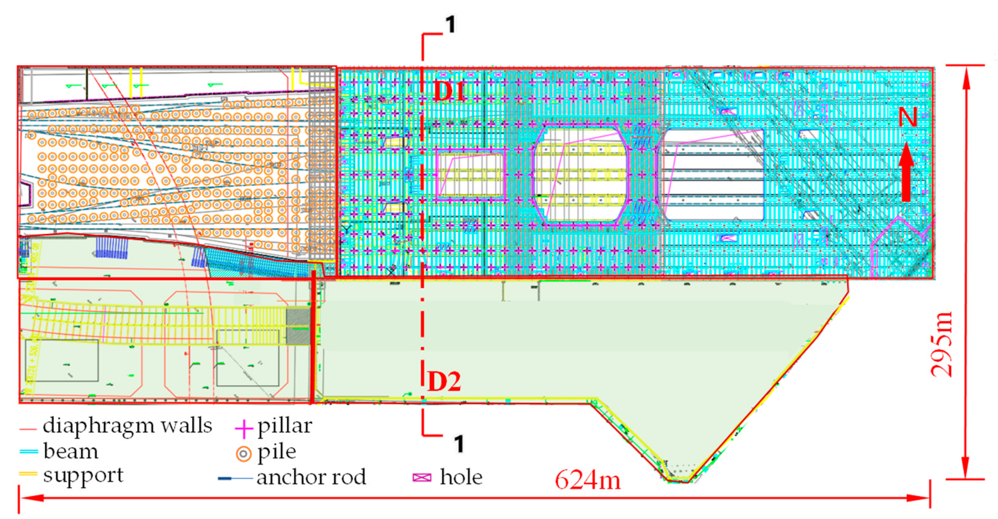
The project is an Integrated Transportation Hub. The foundation pit is approximately 624 m in length and 295 m in width, with a maximum excavation depth of 21.5 m. The underground structure was constructed using the top-down method. For analysis, the excavation was simulated as a plane-strain problem using the 1–1 section. Lateral displacement monitoring points on the north and south diaphragm walls are denoted as D1 and D2, respectively. Figure 4 presents the plan view of the excavation and the location of the analyzed section.
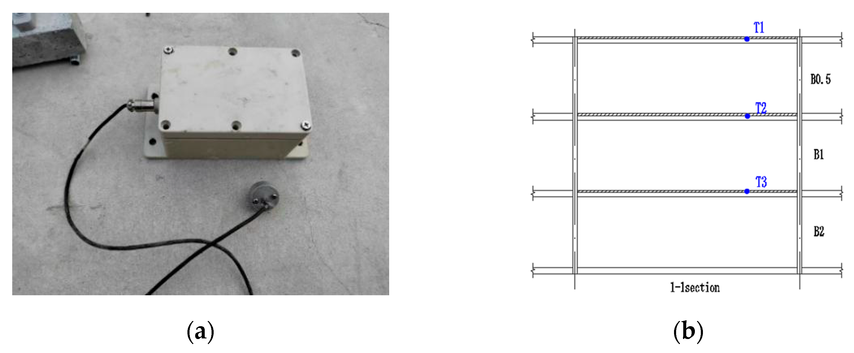
Temperature sensors had a measurement range of −45 °C to 120 °C, with an accuracy of 0.1 °C, and a sampling interval of 20 min. Sensors T1, T2, and T3 were installed at the soffits of the slabs at Levels B0.5, B1, and B2, respectively. The layout of the temperature sensors is shown in Figure 5.
To obtain the vertical temperature gradient of the excavation, monitoring of the temperature field was carried out during the construction period, with continuous observation from September 2024 to February 2025 at a sampling interval of 20 min. The monitoring included measurements of the wall’s top displacement and structural temperature at different depths. Table 1 shows the corresponding temperatures within the different excavation steps. Since excavation was carried out using the top-down method, the sensors could not be installed before the corresponding underground structural components were built; therefore, they were marked as “not arranged.”

2.2. Finite Element Model

The finite element model of the excavation is built by PLAXIS 2D CE V20 [26]. Figure 6 shows the plane-strain finite element model for Section 1–1. The computational size was 1400 m × 310 m. The model comprised 16,308 elements and 244,620 nodes.
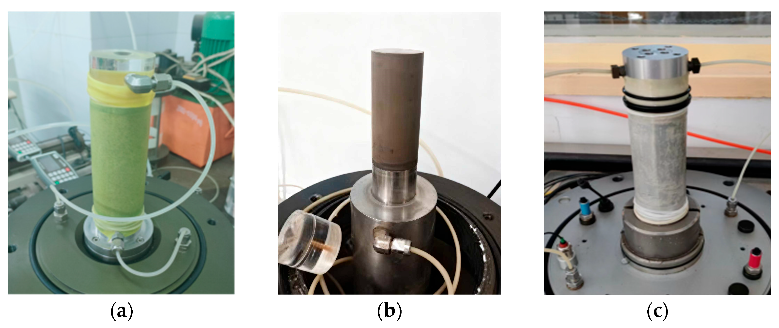
The hardening soil small-strain (HSS) model was used as the constitutive model of the soil. The HSS model assumes that the soil behaves as an elasto-plastic material and that its shear stiffness and compression modulus vary with the stress level. It is an advanced constitutive model that accounts for soil stiffness degradation at small strain levels [27]. The model involves 13 parameters, comprising 11 hardening soil (HS) parameters and 2 small-strain parameters. The reference secant modulus in triaxial compression E 50 ref , the reference oedometer modulus E ur ref , and the reference unloading–reloading modulus E oed ref were obtained from triaxial tests. The small-strain shear modulus G 0 ref and the reference shear strain γ 0.7 were determined from resonant column tests; representative laboratory specimens are shown in Figure 7. The effective cohesion c and effective friction angle φ were derived from site investigation data. The remaining parameters were assigned following prior studies [28,29]: unloading–reloading Poisson’s ratio v ur = 0.20 ; failure ratio R f = 0.9 ; reference pressure p ref = 100   kPa ; stiffness exponent m = 0.5 ; and dilatancy angle ψ = 0 . Table 2 lists the HSS parameters obtained by laboratory tests. In addition, the soil density is also provided in Table 2.
Based on the results of the HSS model calibration, the physical properties of sand and clay show clear differences. The values of E 50 r e f , E u r r e f , E o e d r e f and φ for sand are higher than those for clay, indicating that sand exhibits higher stiffness, lower compressibility, and greater shear strength, mainly governed by interparticle friction. In contrast, clay shows higher c′, reflecting the dominance of electrochemical bonding and structural adhesion between particles. Consequently, clay tends to experience larger plastic deformation and lower stiffness under loading. These differences explain the distinct deformation responses of sandy and clayey strata during excavation.

2.3. Finite Element Analysis Results

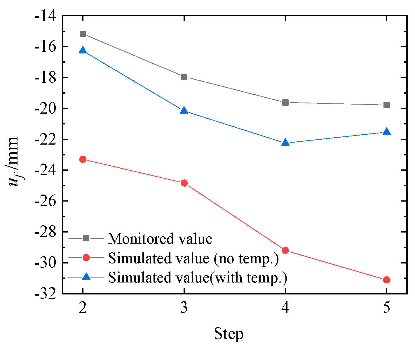
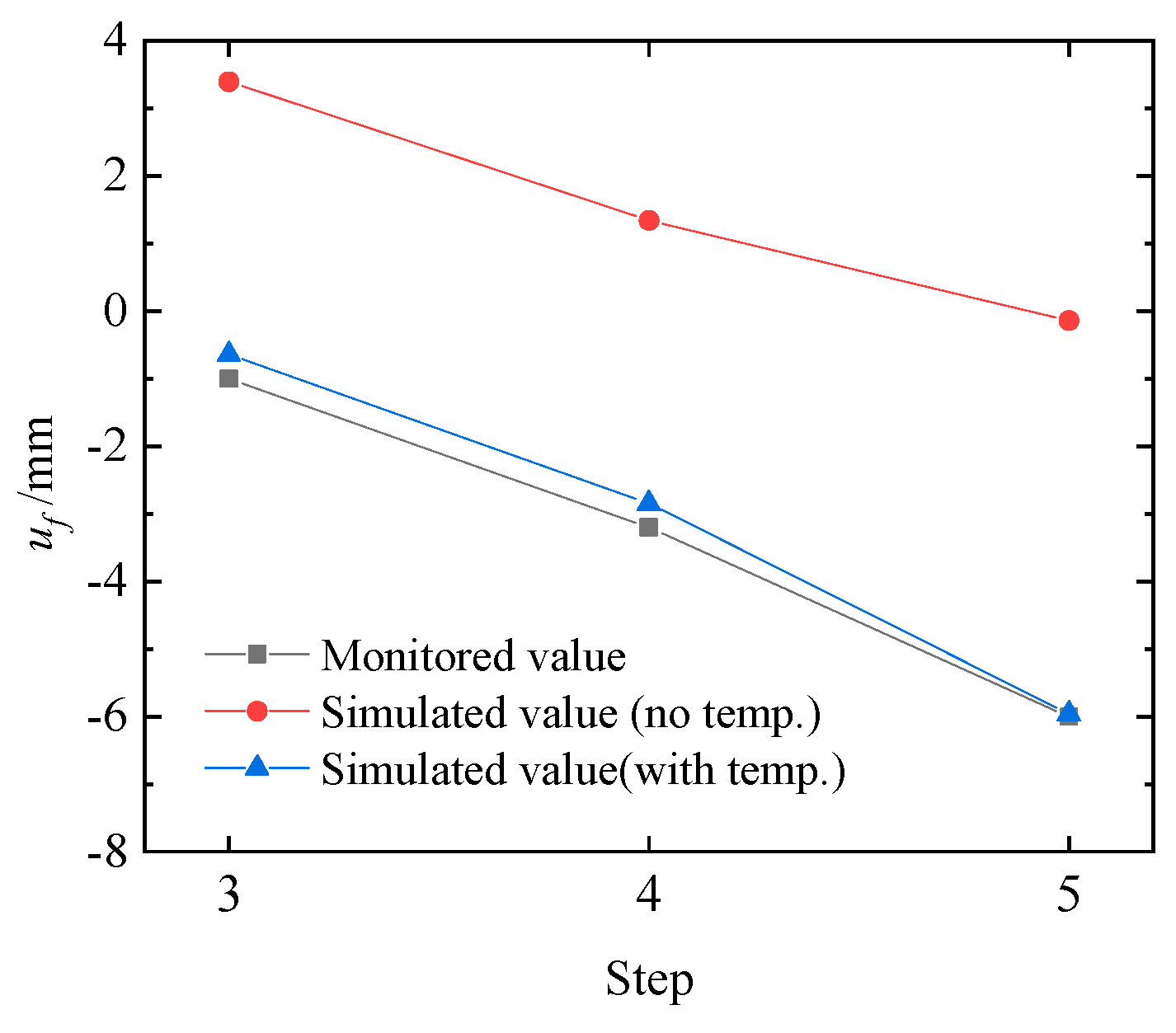
The lateral displacements of the structure were computed with and without temperature effects. Figure 8 and Figure 9 show the monitored and computed displacements for the north (D1) and south (D2) diaphragm walls, respectively. In the figures, positive displacement denotes movement toward the north.
The root mean square error (RMSE) was used to quantify the discrepancy between monitored and calculated displacements, defined as
RMSE = i = 1 n ( Y i Y ^ i ) 2 i = 1 n Y ^ i 2 × 100 %
Here, n is the number of construction steps, Y i and Y ^ i are the calculated and monitored displacements at step i, respectively.
Without considering temperature effects, the simulated displacement at D1 is negative (i.e., the north diaphragm wall moves south), which is consistent in direction with mechanics and with the measurements, but its magnitude is overestimated; the RMSE relative to the observations is 50.2%. At D2, the simulated displacement is positive (the south diaphragm wall moves north), which aligns with mechanics-based expectations but is opposite to the monitored direction, yielding an RMSE of 125.3%. After incorporating temperature effects, the north diaphragm wall still moves south, but the discrepancy from the measurements is markedly reduced (RMSE = 11.1%). Meanwhile, the displacement direction of the south diaphragm wall reverses from northward to southward, consistent with the monitoring results, and the RMSE decreases to 8.49%.
The reason is that, without temperature effects, the model reflects only excavation-induced loading and cannot represent slab deformation driven by ambient temperature, resulting in an opposite displacement direction for the south wall compared with the measurements. When temperature effects are included, thermal expansion of the floor slabs tends to drive the north wall northward and the south wall southward; moreover, because the retained ground/slope height on the north side is 8 m higher than on the south, the north side provides a stronger constraint. Under the combined action of temperature and soil-pressure loading, the south diaphragm wall moves southward, and the computed trends become consistent with the observations. These findings indicate that, for long and large underground structures, monitored displacements during construction must account for seasonal temperature variations.

3. Soil Parameter Inversion Considering Temperature Effects

3.1. Machine Learning Methods for Small-Sample Datasets

During inversion of geotechnical parameters, the amount of available monitoring data and numerical simulation results is typically limited by on-site instrumentation, laboratory testing conditions, and computational cost. As a result, the inversion task commonly constitutes a small-sample learning problem [30]. In addition, the relationship between parameters and responses is nonlinear: the mapping from soil mechanical parameters to excavation-induced displacements and stress fields is governed by nonlinear constitutive behavior, path dependence of staged construction, and multi-factor coupling, and thus cannot be adequately represented by simple linear models. This pronounced nonlinearity constrains the accuracy and applicability of traditional regression approaches. Considering the small sample size and nonlinear characteristics of the inversion problem, three machine-learning algorithms—DT (Decision Tree), RF (Random Forest), and GPR (Gaussian Process Regression)—are employed for parameter inversion.

3.1.1. DT Algorithm

DT is a typical nonparametric supervised learning method that models the mapping between input features and output variables using a tree structure. The method is to recursively select the optimal feature and its split point to partition the sample space into subsets layer by layer, thereby forming a tree-like decision structure. In parameter inversion problems, DT can effectively handle the nonlinear relationship between parameters and displacement responses and offer strong interpretability.
The training sample is set as follows:
S = x i , y i i = 1 , 2 , , N
where x i p denotes the input feature vector of the i-th sample, and yi denotes the corresponding output. Under a candidate splitting feature A, the tree determines the optimal split point by minimizing the post-split impurity. A commonly used impurity measure is the mean squared error (MSE):
MSE ( S ) = 1 S ( x i , y i ) S ( y i y ¯ ) 2
where y ¯ is the mean of the sample set S.
If feature A is split at a threshold s to produce the left and right subsets S left and S right , the corresponding weighted error is as follows:
MSE ( S , A , s ) = | S left | | S | MSE ( S left ) + | S right | | S | MSE ( S right )
The optimal split ( A , s ) is obtained by minimizing the above criterion:
( A , s ) = arg   min A , s MSE ( S , A , s )
Through recursive partitioning until a stopping condition is met (such as maximum depth or minimum number of samples in a leaf node), a tree can be generated. The final prediction value is given by the mean of the training samples that fall into the corresponding leaf node.
The DT algorithm can intuitively capture the nonlinear mapping relationship between input features and output variables, and it imposes few assumptions on data distribution. However, a single decision tree is prone to overfitting, and ensemble learning methods (such as the RF algorithm) are often employed to improve its generalization ability.

3.1.2. RF Algorithm

The RF is a nonparametric method based on the concept of ensemble learning, consisting of multiple decision trees. The method is to reduce the overfitting risk of a single decision tree and improve the model’s generalization ability through “random sampling and multiple tree integration.” For soil parameter inversion problems, the RF can effectively handle nonlinear relationships under small-sample conditions and exhibits strong robustness.
During the training phase, the RF employs the “bootstrap sampling” method to randomly and repeatedly draw several subsample sets from the original dataset S, each used to train a different decision tree. Meanwhile, at each node-splitting stage within a tree, not all features are considered; instead, a subset of candidate features is randomly selected from the input feature set, from which the optimal split point is determined. This “double randomness” mechanism ensures diversity among the trees in the forest, thereby enhancing the overall stability of the model.
During the prediction phase, suppose the forest contains M trees, and the prediction result of the j-th tree is y ^ ( m ) ( x ) ; then, the final output of the RF is obtained by averaging the predictions of all trees:
y ^ ( x ) = 1 M m = 1 M y ^ ( m ) ( x )
The RF algorithm, by integrating multiple decision trees, effectively alleviates the overfitting problem of a single tree. It exhibits strong robustness to outliers and noisy data and can naturally output feature importance indicators, providing a valuable reference for identifying key soil parameters in parameter inversion.

3.1.3. GPR Algorithm

GPR is a nonparametric Bayesian learning method based on probabilistic statistics. It can establish a nonlinear mapping between inputs and outputs under small-sample conditions while providing uncertainty quantification for the predictions. The core idea is to treat the unknown function as a random process that follows a Gaussian process, meaning that for any finite set of input points, the corresponding function values follow a multivariate Gaussian distribution.
Let the training samples be (2). Under the Gaussian process framework, the output y ( x ) can be expressed as follows:
y ( x ) = f ( x ) + ε ,   ε Ν ( 0 , σ n 2 )
where f ( x ) is the latent function and ε is the observation noise. Assume that f ( x ) follows a zero-mean Gaussian process:
f ( x ) G P ( 0 , k ( x , x ) )
where k ( x , x ) is the kernel function used to characterize the correlation between inputs. A commonly used kernel is the radial basis function (RBF) kernel:
k ( x , x ) = σ f 2 exp x x 2 2 l 2
where σ f 2 is the signal variance, and l is the characteristic length scale.
Given the training data, the predicted x output at a new point follows a conditional Gaussian distribution, with its mean and variance expressed as follows:
μ ( x ) = k ( x , X ) K ( X , X ) + σ n 2 I 1 y
σ 2 ( x ) = k ( x , x ) k ( x , X ) K ( X , X ) + σ n 2 I 1 k ( X , x )
where X = x 1 , x 2 , , x N T is the kernel matrix between training samples and K ( X , X ) is the output vector.
The GPR algorithm can achieve stable prediction results under small-sample conditions, making it suitable for soil parameter inversion problems. Employing kernel functions allows us to flexibly characterize the nonlinear relationship between inputs and outputs. Moreover, its output includes both the predictive mean and confidence interval, allowing for a quantitative representation of uncertainty.

3.2. Soil Parameter Inversion

3.2.1. Dataset Preparation

A total of 17 soil layers were identified from the existing geotechnical investigation data, including 10 sandy layers and 7 cohesive soil layers. Owing to the significant differences in physical properties between sand and clay, as well as their alternating distribution within the strata, it is difficult to merge or simplify the layers in large-scale foundation pit simulations. Therefore, the soil layers were divided into a sand group and a clay group.
An orthogonal experimental design table, L27(313), was constructed by combining all parameter levels within each group. The three parameter levels were defined as multiples of the initial values, i.e., 0.8, 1.0, and 1.2 for one group, and 0.9, 1.0, and 1.3 for the other, resulting in a total of 54 sets of soil parameter combinations. Among them, 36 sets were randomly selected as the training dataset, and 18 sets as the testing dataset.
These parameter combinations were input into the temperature-coupled finite element model, yielding 54 samples containing the displacement inputs and corresponding soil parameter outputs for model training.

3.2.2. Model Construction for Training

During model training, the performance of different algorithms largely depends on the proper configuration of their hyperparameters. For the DT algorithm, the key hyperparameters include the maximum tree depth, the minimum number of samples required to split a node, and the minimum number of samples in a leaf node, which help prevent overfitting and ensure an appropriate tree complexity.
For the RF algorithm, in addition to inheriting the relevant parameters of individual decision trees, it is also necessary to determine the number of base learners in the forest, the number of features considered at each split, and whether to use bootstrap sampling, so as to balance model generalization and computational efficiency.
For the GPR algorithm, its performance heavily depends on the choice of kernel function and parameter optimization. It is also necessary to set the noise term to enhance numerical stability and to increase the number of optimizer restarts to improve the global search capability of hyperparameter optimization.
The specific hyperparameter settings for each algorithm are listed in Table 3.
The 54 training samples were input into the machine learning models, with the horizontal displacements of two diaphragm wall monitoring points across seven construction stages serving as inputs, and the 13 soil parameter levels as outputs. Prediction accuracy metrics for the three algorithms were calculated on the validation set, with the results for the test set shown in Figure 10. The RMSE values for DT, RF, and GPR were 6.15%, 5.57%, and 5.83%, respectively, and the corresponding coefficients of determination (R2) were 0.803, 0.846, and 0.822.
These results indicate that all three methods can reasonably fit the sample data to a certain extent, with R2 values greater than 0.80, demonstrating strong explanatory power for the variance of the output variables. Among them, RF achieved the lowest RMSE (5.57%) and the highest R2 (0.846), indicating superior prediction accuracy and generalization performance compared with DT and GPR. This is primarily attributed to RF’s ensemble of multiple decision trees, which effectively reduces the overfitting risk of a single model and enhances the overall robustness of the model.

3.2.3. Analysis of Inversion Results

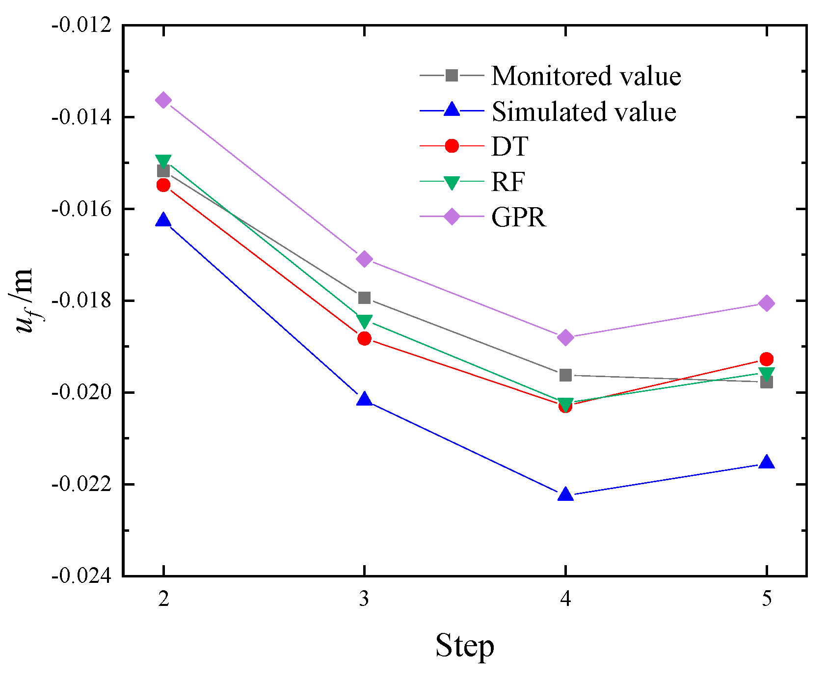
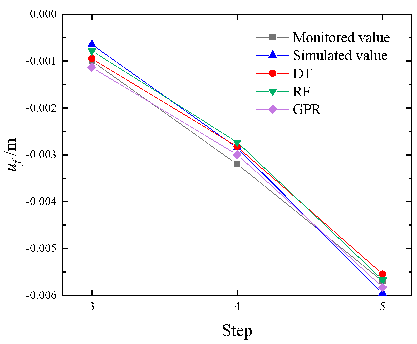
The inverted parameters were input into the model for computation. Figure 11 and Figure 12 show the calculated horizontal displacements of the diaphragm walls ( u f ) after optimizing the soil layer parameters.
The RMSE values for the various methods are summarized in Table 4. It can be seen that after inverting the soil layer parameters using machine learning algorithms, the model accuracy is significantly improved. Specifically, for monitoring point D1, the RF algorithm achieves the highest accuracy with an RMSE of 2.30%, while for monitoring point D2, GPR provides the best optimization with an RMSE of 4.2%. Overall, among the three algorithms, RF demonstrates the highest accuracy, with an average RMSE of 4.23%.

4. Conclusions

This study first investigated the influence of temperature effects on the displacement of underground structures. Based on this, a soil layer parameter inversion method for super-large excavation pits considering temperature effects was proposed. From the experimental and computational results, the following conclusions can be drawn:
  • A method was proposed that accounts for the combined effects of excavation and temperature during the construction of super-large pits, and the results show that temperature is a non-negligible factor in deformation analysis. Compared with previous studies that ignored thermal influences, this work provides a more accurate representation of structural deformation behavior and demonstrates the necessity of considering temperature effects in the design and analysis of deep and large-scale excavations.
  • Soil layer parameter inversion was conducted based on the finite element model incorporating temperature effects. Training samples were constructed using soil layer grouping and orthogonal experimental design, and the accuracy of DT, RF, and GPR machine learning algorithms was compared. Inverting the soil parameters effectively reduced computational errors, with the RF algorithm achieving the lowest error.
Based on these findings, several recommendations can be made for urban excavation projects. Temperature effects should be explicitly incorporated into deformation analysis and design verification for deep and super-large excavations, as ignoring thermal influences may increase the potential risks of excessive wall deformation, ground settlement, or structural instability in urban environments. More accurate soil parameter inversion, supported by temperature-integrated numerical modeling and data-driven methods, can help reduce deformation prediction errors and enhance the safety and reliability of excavation support systems. Therefore, the proposed framework provides practical guidance for improving deformation control, mitigating engineering risks, and optimizing design in urban deep excavation engineering.
However, the monitoring period was relatively short and limited to a single project, which may not fully capture long-term and regional variability. Future research should extend the monitoring duration, consider more complex environmental factors such as groundwater variation, and explore advanced algorithms to further improve the accuracy and general applicability of the proposed framework.

Author Contributions

D.L.: Conceptualization, Investigation. X.S.: Formal analysis, Investigation, Methodology, Validation, Writing—original draft and editing. D.P.: Methodology, Conceptualization, Writing—review. All authors have read and agreed to the published version of the manuscript.

Funding

This research was funded by the National Natural Science Foundation of China grant number 52478121.

Institutional Review Board Statement

Not applicable.

Informed Consent Statement

Not applicable.

Data Availability Statement

The data that support the findings for this study are available from the authors by request.

Conflicts of Interest

Author Dong Liu was employed by the company Beijing Uni.-Construction Group Co., Ltd. The remaining authors declare that the research was conducted in the absence of any commercial or financial relationships that could be construed as a potential conflict of interest.

Abbreviations

The following abbreviations are used in this manuscript:
PSOParticle Swarm Optimization
HSSHardening Soil Small Strain
DTDecision Tree
RFRandom Forest
GPRGaussian Process Regression

References

  1. Tang, L.; Liao, S.; Yang, Y.; Fan, Y.; Liu, Z. A Spatiotemporal Data Mining Method for Advanced Prediction and Assessment of Large Combined Excavation-Induced Wall Deformations and Risks. J. Rock Mech. Geotech. Eng. 2025, 17, 2758–2777. [Google Scholar] [CrossRef]
  2. Johari, A.; Pourbeirak, S. Impact of Soil Heterogeneity on Stochastic SANISAND Constitutive Model and Static Liquefaction Potential. Iran. J. Sci. Technol. 2025, 49, 5003–5020. [Google Scholar] [CrossRef]
  3. Marquardt, D.W. An Algorithm for Least-Squares Estimation of Nonlinear Parameters. J. Soc. Ind. Appl. Math. 1963, 11, 431–441. [Google Scholar] [CrossRef]
  4. Levenberg, K.A. Method for the Solution of Certain Non-Linear Problems in Least Squares. Q. Appl. Math. 1944, 2, 164–168. [Google Scholar] [CrossRef]
  5. Sacks, J.; Welch, W.J.; Mitchell, T.J. Design and Analysis of Computer Experiments. Stat. Sci. 1989, 4, 409–423. [Google Scholar] [CrossRef]
  6. Goldberg, D.E. Genetic Algorithms in Search, Optimization, and Machine Learning; Addison-Wesley: Reading, MA, USA, 1989. [Google Scholar]
  7. Kennedy, J.; Eberhart, R. Particle Swarm Optimization. In Proceedings of the ICNN′95—International Conference on Neural Networks, Perth, WA, Australia, 27 November–1 December 1995; pp. 1942–1948. [Google Scholar] [CrossRef]
  8. Goh, A.T.C. Empirical Design in Geotechnics Using Neural Networks. Géotechnique 1995, 45, 709–714. [Google Scholar] [CrossRef]
  9. Cheng, Q.; Yang, Z.; Qin, S. Application of Soil Parameters Inversion Based on PSO-MLSSVR in Deep Foundation Pit Engineering. J. Eng. Geol. 2022, 30, 520–532. [Google Scholar] [CrossRef]
  10. Ji, H.; Jin, Y.; Yin, Z. Enhancement of Genetic Algorithm and Its Application to the Identification of Soil Parameters by Inverse Analysis. Chin. J. Comput. Mech. 2018, 35, 224–229. [Google Scholar] [CrossRef]
  11. Cao, J.; Tang, B.; Li, H. Optimization of LS-SVM Based on SA-PSO Algorithm for Inversion of Equivalent Parameters of Foundation Soil Layers. Ind. Saf. Environ. Prot. 2023, 49, 15–20. [Google Scholar]
  12. Zhao, C. A Modified Back Analysis Method for Deep Excavation with Multi-Objective Optimization Procedure. J. Rock Mech. Geotech. Eng. 2024, 16, 1373–1387. [Google Scholar] [CrossRef]
  13. Liu, M.; Zhuang, P.; Lai, F. A Bayesian Optimization-Genetic Algorithm-Based Approach for Automatic Parameter Calibration of Soil Models: Application to Clay and Sand Model. Comput. Geotech. 2024, 176, 106717. [Google Scholar] [CrossRef]
  14. Li, B.Y.; Sima, J. Horizontal Displacement Back-Analysis for Deep Excavation Using MEC-BP Neural Network. J. Railw. Sci. Eng. 2021, 18, 1764–1772. [Google Scholar]
  15. Liu, W.; Tong, L.; Li, H.; Wang, Z.; Sun, Y.; Gu, W. Multi-Parameter Intelligent Inverse Analysis of a Deep Excavation Considering Path-Dependent Behavior of Soils. Comput. Geotech. 2024, 174, 106597. [Google Scholar] [CrossRef]
  16. Sun, L.; Liu, S.; Zhang, L.; He, K.; Yan, X. Prediction of the Displacement in a Foundation Pit Based on Neural Network Model Fusion Error and Variational Modal Decomposition Methods. Measurement 2025, 240, 115534. [Google Scholar] [CrossRef]
  17. Hu, H.; Tian, Y.; Zheng, N.; Du, X.; Guo, H.; Xu, Z. Numerical Simulation on an Ultra-Large Seven-Ring Internal Support System Considering the Effects of Soil–Structure Interaction and Temperature. Buildings 2025, 15, 463. [Google Scholar] [CrossRef]
  18. Yang, J.; Cui, F.; Zhang, Y.; Li, B.; Li, B.; Mei, W. Influence of Seasonal Ambient Temperature on the Temperature and Deformation Behaviors of Underground Utility Tunnels. Soil Mech. Found. Eng. 2025, 62, 253–260. [Google Scholar] [CrossRef]
  19. Ji, F.; Shi, S. Temperature Effect Analysis of Mechanical Behavior of Deep Foundation Pit Supporting Structure. Chin. J. Undergr. Space Eng. 2024, 20, 298–309. [Google Scholar]
  20. Park, S.; Son, Y.; Kim, J.; Won, D.; Choi, H. Thermal and Mechanical Impact of Artificial Ground-Freezing on Deep Excavation Stability in Nakdong River Deltaic Deposits. Eng. Geol. 2024, 343, 107796. [Google Scholar] [CrossRef]
  21. Lu, P.; Han, L.; Yu, Y. Finite Element Analysis of Temperature Stress in Strut of Foundation Pit. Rock Soil Mech. 2008, 29, 1290–1294. [Google Scholar]
  22. Liu, C.; Zhang, Y.; Zheng, G. Effects of Seasonal Temperature Change on a Large-Excavation Project. Chin. J. Geotech. Eng. 2016, 38, 627–635. [Google Scholar] [CrossRef]
  23. Wang, X.; Li, M.; Chen, J.; Zhu, Y. Performance of a Deep Excavation with the Composite Retaining Wall Using Artificial Ground Freezing Method. Cold Reg. Sci. Technol. 2022, 204, 103676. [Google Scholar] [CrossRef]
  24. Luo, Y.; Zhao, L.; Zhu, L.; Tian, F.; Lei, K.; Sun, A. Land Subsidence Characteristics and Disaster Prevention in the Tongzhou Area, Beijing. PIAHS 2020, 382, 715–722. [Google Scholar] [CrossRef]
  25. Zhang, M.; Li, W.; Yan, Q.; Zhang, M.; Liang, W. The Research on 3D Modelling and Visualization of the Quaternary in Tongzhou Area, Beijing. Geo-Spat. Knowl. Intell. 2018, 848, 3–12. [Google Scholar] [CrossRef]
  26. Bentley PLAXIS 2D Materials Models Manual. Available online: https://files.seequent.com/PLAXIS/Manuals/PLAXIS_2D/English/PLAXIS_2D_3_Material%20Models%20Manual.pdf (accessed on 16 November 2025).
  27. Hu, J.; Du, Q. Parameter Study and Engineering Verification of the Hardening Soil Model with Small-Strain Stiffness for Loess in the Xi’an Area. Appl. Sci. 2025, 15, 1278. [Google Scholar] [CrossRef]
  28. Li, M.; Chen, H.; Zhang, Z.; Chen, J. Numerical Analysis of a Deep and Oversized Group Excavation: A Case Study. Undergr. Space 2025, 21, 178–197. [Google Scholar] [CrossRef]
  29. Kawa, M.; Puła, W.; Truty, A. Probabilistic Analysis of the Diaphragm Wall Using the Hardening Soil-Small (HSs) Model. Eng. Struct. 2021, 232, 111869. [Google Scholar] [CrossRef]
  30. Hu, H.; Luo, X.; Wang, W.; Xu, C.; Zheng, G. Soil Parameter Inversion Modeling Using Deep Learning Algorithms and Its Application to Settlement Prediction: A Comparative Study. Acta Geotech. 2023, 18, 4703–4720. [Google Scholar] [CrossRef]
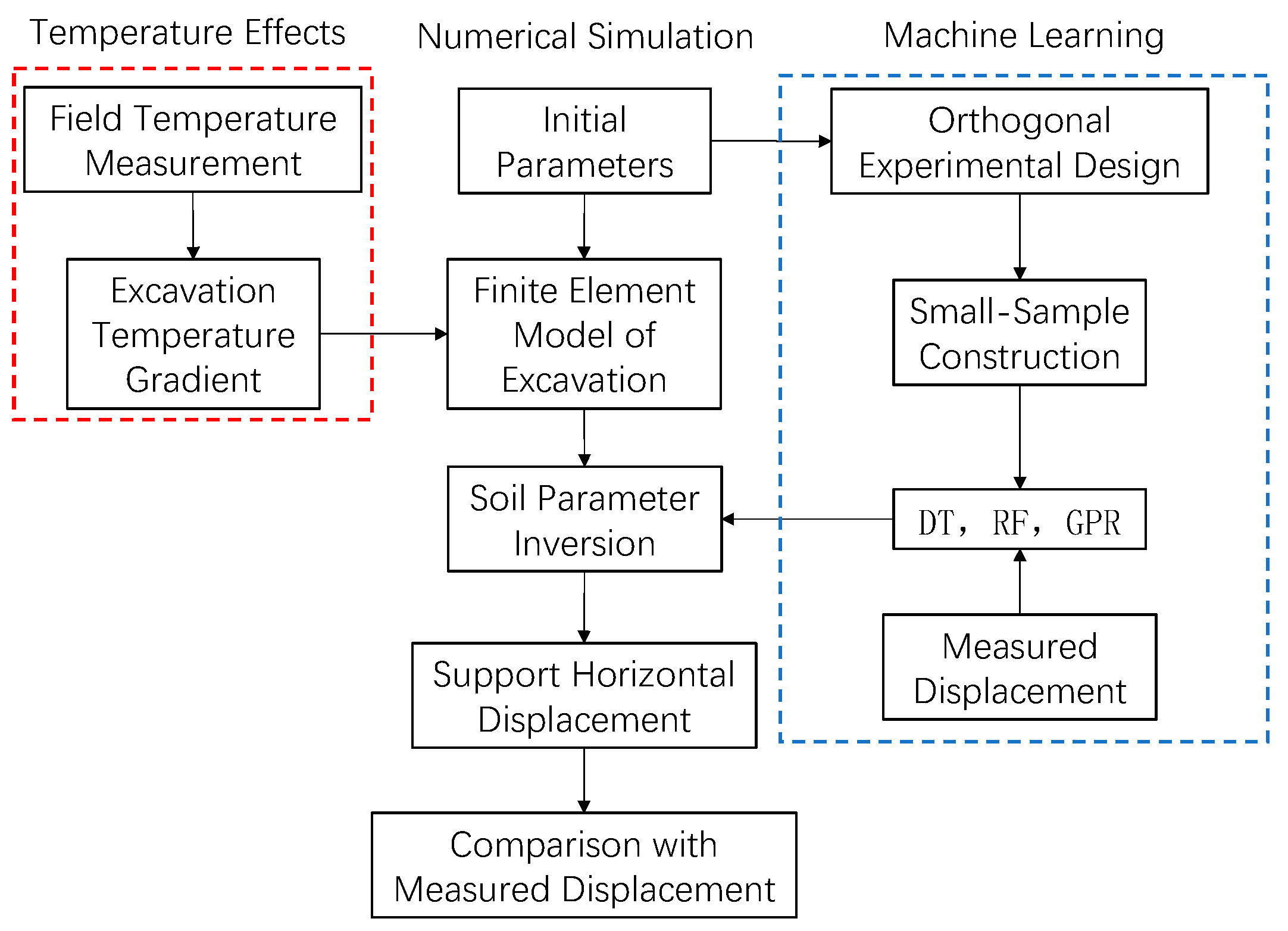
Figure 1. Research flowchart.
Applsci 15 12511 g001
Figure 2. Map of Tongzhou District, Beijing.
Applsci 15 12511 g002
Figure 3. Stratigraphic distribution.
Applsci 15 12511 g003
Figure 4. Plan view of the excavation and location of Section 1–1.
Applsci 15 12511 g004
Figure 5. Temperature acquisition system: (a) temperature sensor; (b) sensor installation locations.
Applsci 15 12511 g005
Figure 6. Finite element model of the excavation.
Applsci 15 12511 g006
Figure 7. Prepared soil specimens: (a) fine sand; (b) silty clay; (c) specimens for resonant column testing.
Applsci 15 12511 g007
Figure 8. Displacement at D1.
Applsci 15 12511 g008
Figure 9. Displacement at D2.
Applsci 15 12511 g009
Figure 10. Validation results on the test set.
Applsci 15 12511 g010
Figure 11. Inverted horizontal displacement of D1.
Applsci 15 12511 g011
Figure 12. Inverted horizontal displacement of D2.
Applsci 15 12511 g012
Table 1. Excavation deformation and vertical temperature field.
Construction StepDescriptionD1 (m)D2 (m)T1 (°C)T2 (°C)T3 (°C)
step 1B0.5 slab construction
step 2Local excavation to 8 m; B0.5 excavation; B1 slab construction−0.01517Not arranged30Not arrangedNot arranged
step 3Overall excavation to 12 m; completion of B1 excavation; B2 slab construction−0.01794−0.0012622Not arranged
step 4B2 excavation to 50%; installation of B2 raking struts−0.01962−0.00322723Not arranged
step 5Excavation to 22 m; completion of B2 excavation; B2 base slab construction−0.01977−0.00572924.522.5
Table 2. HSS model parameters.
Soil TextureLayer Thickness (m) E 50 r e f (MPa) E o e d r e f
(MPa)
E u r r e f (MPa) c (kPa) φ γ 0.7
(×10−4)
G 0 r e f
(MPa)
ρ
kg/m3
sandy silt3.110.49.492.32102.0012015.50
clayey silt7.110.49.492.31523.62.0012019.03
fine sand4.118.911.182.12282.0010715.43
fine sand521.212.592.42323.0012016.98
fine sand5.925.414.91112323.0014416.98
silty clay5.5511.09.9797.735103.0012720.35
fine sand7.0533.819.91472343.0019120.21
silty clay5.4916.414.914659163.0019019.49
fine sand4.6142.124.81832353.0023820.4
fine sand8.0251.330.22232363.0029020.4
silty clay3.4820.718.818455143.0023919.72
fine sand11.761.236.02662363.0034620.6
silty clay2.624.422.22185514.43.0028319.52
fine sand8.869.741.03032363.0039420.60
silty clay8.3625.122.82237719.73.0029019.94
silty clay4.3628.626.02557915.23.0033119.82
fine sand214.9889.852.83912383.0050820.60
Table 3. Key hyperparameter settings for the algorithms.
AlgorithmsTraining ParameterValue
DTMaximum Depth5
Minimum Samples to Split a Node3
Minimum Samples per Leaf Node2
RFNumber of Base Learners120
Number of Features per Split14
Bootstrap SamplingTrue
GPRKernel FunctionRBF
Noise Term 10 3
Number of Optimizer Restarts4
Table 4. RMSE values for different machine learning algorithms.
Monitoring PointSimulated ValueDTRFGPR
D111.10%3.41%2.30%7.11%
D211.00%7.80%6.16%4.20%
Mean value11.05%5.61%4.23%5.65%
Disclaimer/Publisher’s Note: The statements, opinions and data contained in all publications are solely those of the individual author(s) and contributor(s) and not of MDPI and/or the editor(s). MDPI and/or the editor(s) disclaim responsibility for any injury to people or property resulting from any ideas, methods, instructions or products referred to in the content.