Article

Numerical Study on the Aerodynamic and Structural Response Characteristics of a High-Altitude Wind-Capturing Umbrella

1
College of Aerospace Engineering, Nanjing University of Aeronautics and Astronautics, Nanjing 210016, China
2
CAS Laboratory of Wind Energy Utilization, Institute of Engineering Thermophysics, Chinese Academy of Sciences, Beijing 100190, China
*
Author to whom correspondence should be addressed.
Appl. Sci. 2025, 15(22), 12161; https://doi.org/10.3390/app152212161
Submission received: 16 October 2025 / Revised: 11 November 2025 / Accepted: 13 November 2025 / Published: 16 November 2025
(This article belongs to the Section Aerospace Science and Engineering)

Abstract

As global demand for renewable energy continues to grow, high-altitude wind energy, characterized by high speed, wide distribution, and strong stability, has emerged as a promising alternative to low-altitude wind energy. Airborne Wind Energy systems (AWEs) are key to harnessing high-altitude wind, and Ground-Generator (Ground-Gen) AWEs are favored for their lower costs and simpler deployment. This study focuses on the umbrella–ladder-type Ground-Gen AWEs, aiming to address the research gap by exploring the influence of canopy permeability on the aerodynamic and structural response characteristics of flexible wind-capturing umbrellas. A single-umbrella model of the high-altitude wind-capturing umbrella was established, and bidirectional fluid–structure interaction (FSI) numerical simulations were conducted using the Arbitrary Lagrangian–Eulerian (ALE) method. Simulations were performed under a 30° angle of attack with two canopy thicknesses (5 × 10⁻⁵ m and 1 × 10⁻⁴ m) and varying permeability (adjusted via viscosity coefficient a and inertial coefficient b). Results showed that higher permeability (smaller a and b) hindered upper canopy inflation, while lower permeability promoted full inflation and more uniform stress distribution. The max/min in-plane shear stress for the model with the lowest permeability (Model F) was approximately 85% lower than that of the model with the highest permeability (Model A). The tension coefficient increased with decreasing permeability. Full inflation resulted in a slightly higher axial load in the upper suspension lines due to the lift force, with a difference of up to 92.3% during slight collapse. This difference becomes significantly more pronounced during severe collapse. Asymmetric flow fields at a 30° attack angle generated a lift force, resulting in higher tension coefficients than those at a 0° attack angle. These findings provide valuable references for the design and optimization of high-altitude wind-capturing umbrellas.

1. Introduction

In recent years, with the ever-increasing global demand for energy, the development of renewable energy has garnered widespread societal attention. Among them, wind energy has emerged as one of the most rapidly expanding industries worldwide, owing to its advantages of being clean, highly efficient, and having low maintenance costs [1]. Early utilization of wind energy resources primarily focused on low-altitude winds, such as those harnessed by wind turbines, with extensive aerodynamic research conducted on their blades [2]. However, low-altitude wind power generation faces some critical challenges, including excessive land area requirements, susceptibility to environmental interference from ground-based activities and structures, and low power generation efficiency due to low wind speeds [3]. High-altitude wind energy is characterized by high wind speed, widespread distribution, high stability, and year-round availability, making it an ideal and efficient green new energy source compared to low-altitude wind energy [4,5]. Particularly, wind energy resources are abundant at altitudes ranging from 500 to 12,000 m, with wind energy density increasing with altitude [6]. If these wind energy resources can be effectively harnessed, they would be sufficient to meet the global energy demand [7], indicating immense development potential.
AWEs represent a primary technology for capturing wind energy to achieve wind power generation. In 1980, Loyd first proposed the concept of large-scale power generation based on “kites” [8]. Nowadays, AWEs can be classified into two types: Ground-Gen AWEs and Fly-Generator (Fly-Gen) AWEs, based on their wind energy capture mechanisms and energy conversion methods [9,10]. Ground-Gen AWEs position generators on the ground, where flight components, driven by wind, move cables to pull the ground-based generators for power generation [11,12,13]. Fly-Gen AWEs position generators on aircraft, where airflow drives them to generate power, then transmits it to the ground via cables. In this case, the working components are typically the aircraft [14,15,16].
Ground-Gen AWEs typically use kites or planar circular parachutes as their primary components. The KitePower team developed 20 KW and 100 KW AWEs in 2007 and 2018, respectively, and successfully deployed them, reaching a peak power of up to 180 KW with an annual output of 450 MW. The system is compact and easy to deploy, but it remains an experimental project rather than a fully commercial one [11]. KiteGen built the first large-scale power plant, the “KiteGen Stem,” with an installed capacity of 3 MW. Their Ground-Gen AWEs occupy relatively small areas and have low power generation costs [12]. Ockels proposed a multi-kite system called Laddermill, which improves wind energy capture by tethering multiple kites in series with cables, thereby increasing power efficiency while maintaining the same footprint [13].
The umbrella–ladder-type Ground-Gen AWEs represent an innovative approach to high-altitude wind power generation. By integrating aerial, traction, and ground components, this system effectively captures and converts wind energy [17]. Li [18] created a rigid-body model for the high-altitude umbrella–ladder system and used Fluent to simulate its response to wind loads at high altitude, obtaining the tension and speed responses of the umbrella–ladder assembly. Luo et al. [19] developed a multi-rigid-body model for the umbrella–ladder-type Ground-Gen AWEs. They achieved error convergence between the actual and desired motion trajectories under longitudinal disturbances in high-altitude wind fields by adjusting the effective wind-facing area of the umbrellas.
It should be emphasized that, currently, there is limited research on numerical simulations of flexible high-altitude wind-capturing umbrellas in aerial ladder systems, especially regarding the effects of permeability on their aerodynamic and structural response characteristics. Previous studies on parachute models primarily focused on their drag characteristics as an effect of a deployable aerodynamic decelerator that inflates and expands by relying on relative motion to the air. For instance, Zhang et al. [20] applied the immersed boundary method to simulate the fluid–structure interaction of parachute inflation processes. They analyzed the inflation dynamics for various typical parachute configurations. Taguchi et al. [21] performed tests in a supersonic wind tunnel using flexible parachutes featuring hemispherical canopy structures, revealing that enhancing canopy permeability reduced both the parachute’s drag coefficient and drag fluctuations. Xu et al. [22] carried out numerical simulations employing a rigid Mars parachute model, exploring the impacts of canopy thickness and relative permeability on aerodynamic characteristics under different Mach number conditions. The results showed that both canopy thickness and relative permeability significantly affected the stability and drag performance of the parachute. Yang et al. [23] developed a new model to simulate how porous canopy permeability impacts the aerodynamic performance of supersonic parachutes, revealing that higher permeability decreased both the average drag coefficient and oscillation amplitude. Yu et al. [24] used a seven-hole probe to measure and analyze the flow field around parachutes under different permeability conditions in wind tunnel tests, discovering that permeability substantially influenced the static pressure difference across the canopy, the convergence point of wake streamlines, stability, and noise.
The studies mentioned above have established a solid foundation for researching the permeability of high-altitude umbrella–ladder-type flexible wind-capturing umbrellas. Building on this, this paper proposes conducting a two-way fluid–structure interaction (FSI) numerical simulation study on the air permeability of high-altitude flexible wind-catching umbrellas. Various FSI numerical simulation methods are used for parachutes, such as IBM [25], CESE, and ALE. The ALE method, a well-established and relatively well-developed method, integrates the strengths of Lagrangian and Eulerian techniques, thereby facilitating the handling of fluid–structure interaction and significant deformation issues. Guan et al. [26] employed the ALE approach to simulate and analyze parachutes featuring radial and circumferential reefing techniques, and compared the findings with airdrop test results. Huang et al. [27,28] investigated the impact of angular air vents and exhaust flow deflectors on the maneuverability of cross parachutes, as well as the influence of suspension line deflection and reefing on the maneuverability of ring-sail parachutes, all based on the ALE method. Cao et al. [29] proposed an ALE-based computational method for controlling the force of parafoils, investigating the coupling mechanism and dynamic variation patterns of control forces under airdrop conditions. Hou et al. [30] employed the ALE approach to conduct numerical simulations of the fully inflated states of no-swinging and free-to-swing cross parachutes under varying Reynolds numbers. They carried out a detailed investigation into the aerodynamic and motion characteristics of these parachutes. Li et al. [31] conducted numerical simulations and experimental validations of the inflation process for underwater parachutes using the ALE method, investigating the impact of parameters such as permeability on the inflation performance of the underwater parachute. The aforementioned research has demonstrated that the ALE method can effectively simulate large deformation fluid–structure interaction problems involving parachute canopies.
The literature review indicates that the umbrella, as an effective deployable aerodynamic decelerator, typically operates at a minimal angle of attack. This contrasts with that in the Ground-Gen AWEs, which require higher angles of attack to capture wind energy efficiently. This paper develops a unified system model for a high-altitude wind-catching umbrella. Using the ALE method, a numerical simulation of fluid–structure interaction is carried out on the high-altitude wind-catching umbrella. The study examines how permeability variations influence the umbrella’s structural response under two different canopy thicknesses when operating at a 30° angle of attack, aiming to provide valuable insights for designing and optimizing high-altitude wind-capturing umbrellas in umbrella–ladder-type Ground-Gen high-altitude wind power generation technology.

2. Methodology

2.1. Governing Equations

Given the low flow velocity, air can be treated as an incompressible fluid. Define the boundary of the fluid domain f as Γf, while the boundary of the structural domain s as Γs.

2.1.1. Fluid Dynamics

Under the ALE method, the time derivative of the fluid field variable f can be expressed as
f X i , t t = f x i , t t + v i w i f x i , t
where Xi and xi represent Lagrangian coordinates and ALE coordinates, respectively; vi and wi represent material velocity and grid velocity, respectively. It can be seen from the above equation that both Lagrangian and Eulerian forms are exceptional cases of ALE description. When material velocity equals grid velocity, it transitions to Lagrangian description; when grid velocity remains zero, it transitions to Eulerian description.
Under the ALE framework, the Navier–Stokes equations are expressed as [32,33]
ρ f t = ρ f v i x i v i w i ρ f x i
ρ f v i t = σ i j , j + ρ f f i ρ f v j w j v i x j
ρ f e t = σ i j v i , j + ρ f f i v i ρ f v j w j e x j
where ρf represents the fluid density, fi stands for the body force, and e signifies specific internal energy. The stress tensor σij is given by
σ i j = p δ i j + μ v i , j + v j , i
where µ represents the fluid’s dynamic viscosity, p is the fluid pressure, and δij is the Kronecker delta function. The corresponding Dirichlet and Neumann boundary conditions are specified as
v i = v i D       o n   Γ f D
σ i j n = 0       o n   Γ f N

2.1.2. Structure Dynamics

The suspension lines are represented through a discrete beam model, with the lines starting in an untensioned state. The governing equation is as follows:
F = K max ( l , 0 ) ,   l = l l 0
where l0 represents the initial length of the line, l denotes the current length of the line, and K is the stiffness defined as follows:
K = E A l 0
where E represents the Young’s modulus, and A is the cross-sectional area.
The canopy structure is a flexible body that undergoes significant deformation during inflation. To avoid computational difficulties caused by severe mesh distortion resulting from large deformations, the Lagrange description is employed for the structural dynamics equations. Its equations of motion are as follows:
ρ s d v s d t = σ i j , j + ρ s f i       i n   s
where vs is the velocity of the structural grid, ρs is the structural density. The canopy is divided into two-dimensional membrane elements. Each element possesses only in-plane stiffness and lacks bending stiffness. Only in-plane tensile stress is considered, while compressive stress is ignored. Initially, there is no stress or strain.

2.2. Fluid–Structure Interaction

In FSI calculations, the canopy structure element is described using the Lagrangian method, while the fluid element employs the ALE method. Coupling between the two is achieved through a penalty function. Both the fluid field and canopy control equations are discretized using a second-order accurate central difference time-stepping method. At the next time step, the positions and velocities of each node are as follows [34]:
x n + 1 = x n + Δ t u n + 1 / 2
u n + 1 / 2 = u n 1 / 2 + Δ t M 1 F i n n + F e x n
where x denotes the displacement vector, u denotes the velocity vector, Fin and Fex represent the internal and external force vectors, respectively, and M is the mass diagonal matrix.
In the penalty function coupling calculation, “spring force” is employed to simulate the interface force. Fluid nodes serve as master nodes, while canopy structure nodes act as slave nodes. If the two nodes do not contact and penetrate each other, no action is taken. When the two nodes contact and penetrate, they experience an equal and opposite interface force proportional to the penetration distance d, defined as follows:
F = k d
where k is the stiffness factor based on the characteristics of the master and slave node mass model, the penetration depth d is defined as follows:
d = v m v s   d t
where vm and vs represent the speed of the master and slave node, respectively.
The FSI process involves alternating solutions between the fluid and structural solvers, with relevant physical quantities transferred through the coupling interface. The Lagrangian structure’s boundary positions and velocities are input to the fluid solver as boundary conditions. The fluid domain is solved using the ALE method to obtain the interfacial forces at the coupling interface. These forces are subsequently applied to the structure, serving as boundary conditions for the structural solver to resolve the dynamic equations. Subsequently, the mesh is updated to begin the next time step of the solution. The general workflow is illustrated in Figure 1.

2.3. Canopy Permeability

The canopy of the high-altitude wind-capturing umbrella is made of flexible porous medium material. Its flexible deformation causes changes in the distribution of the fabric’s pore space structure. Different porosities result in varying permeability of the canopy. Additionally, changes in parameters such as the density and Young’s modulus of the flexible canopy fabric also led to alterations in fluid field parameters, thereby affecting the canopy’s permeability. Based on Ergun’s formula derived from porous media theory, the relationship between the pressure difference across the canopy and its permeability is as follows [35]:
Δ P L = 150 ( 1 ε ) 2 ε 3 μ V D 2 + 1.75 ( 1 ε ) ε 3 ρ V 2 D
where △P is the pressure difference across the porous medium, µ is the viscosity of fluid, ρ is the density of fluid, D is the characteristic length representing the pore size in the permeable medium, L is the thickness of the medium, ε is the relative air permeability of the porous medium, V is the air permeability, equivalent to the rate at which air flows perpendicular to the fabric under this pressure difference.
Assuming the canopy material has constant porosity and the incoming flow has defined viscosity and density, Equation (15) can be expressed as follows [36]:
Δ P L = a V + b V 2
where a and b represent the viscosity coefficient and inertia coefficient of the canopy material, respectively.
Once the canopy is fully inflated and stabilized, its drag coefficient and canopy diameter no longer exhibit significant variation and converge, thereby yielding its post-stabilization structural response. This study employs the double-precision solver LS-DYNA R14 with MMP capability on a 92-core workstation to conduct FSI simulations. These simulations investigate the impact of permeability variations on structural response for a high-altitude wind-capturing umbrella at a 30° angle of attack, under two distinct canopy thickness conditions.

2.4. Model Assumptions

Considering the complex physical characteristics of the canopy deployment process, the computational model used is assumed to be as follows:
  • The initial shape of the canopy is a flat circular shape, with no initial fabric prestress, ignoring the influence of fabric friction on the structural mechanical behavior.
  • The suspension line is in an approximately straightened state, ignoring the aerodynamic force acting on the suspension line and the cable line.
  • Only studying the aerodynamic effects of the canopy, ignoring the potential collision between the canopy and the cable, and using a bracket instead of the cable to restrict the movement of the canopy.
  • In the flow field model, the velocity direction of the fluid is constant, and the velocity of 15 m/s remains unchanged. The fluid is incompressible.
  • The inflation process of the canopy is an infinite mass situation, ignoring the influence of gravity.

3. High-Altitude Wind-Catching Umbrella Model

3.1. Geometric and Finite Element Model

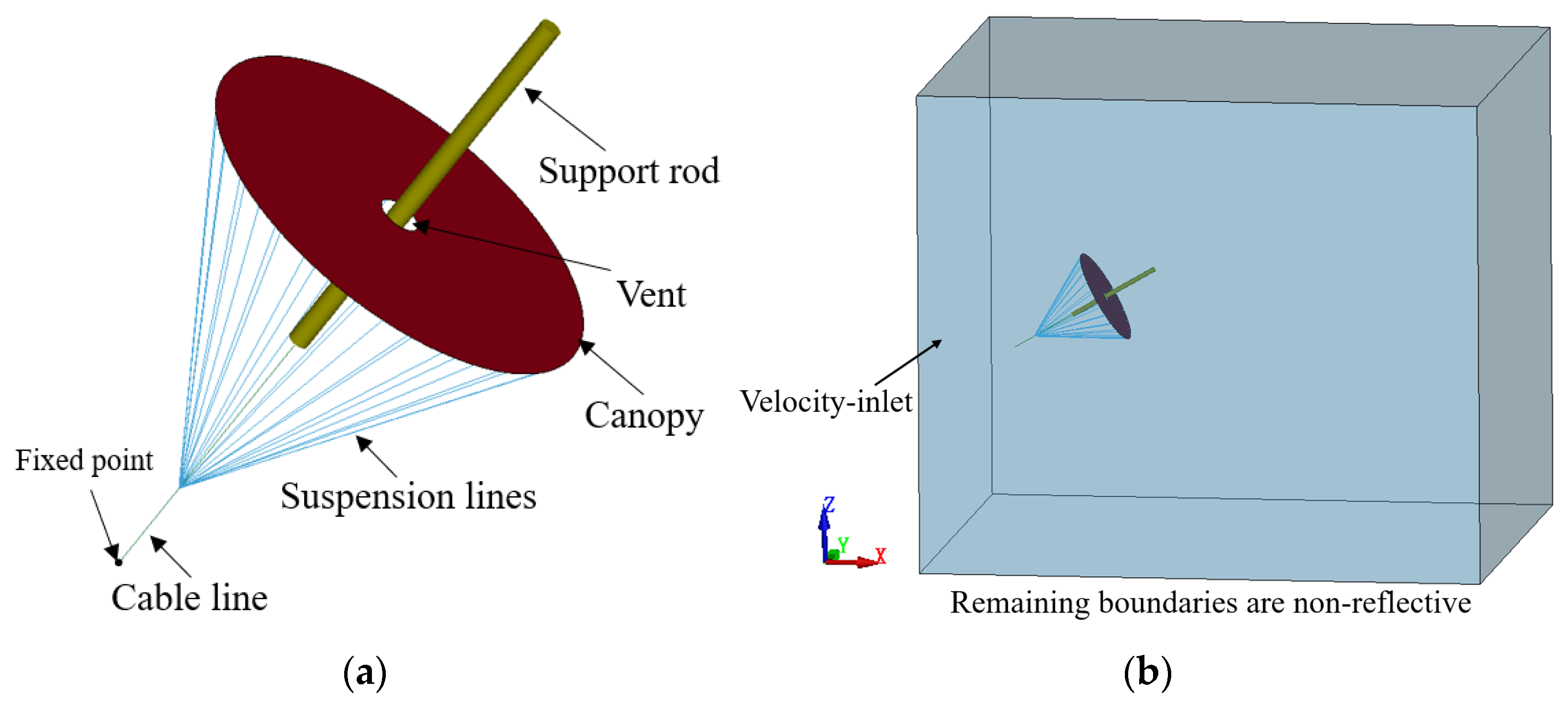
This paper utilizes a planar circular canopy, commonly employed in parachute systems, as the canopy for the high-altitude wind-capturing umbrella system. The canopy consists of 12 gores and 24 suspension lines. A simplified model of the high-altitude wind-capturing umbrella system is shown in Figure 2. It comprises the canopy, suspension lines, cable, and support rod. The cable is fixed at its lower end, and the support rod is anchored to restrict the angle of the wind-capturing umbrella. The cable fixed point is located 2 m from the suspension lines knot, while the base of the support rod is positioned 3.93 m from the suspension lines knot. Table 1 gives the specific geometric parameters of the structure.
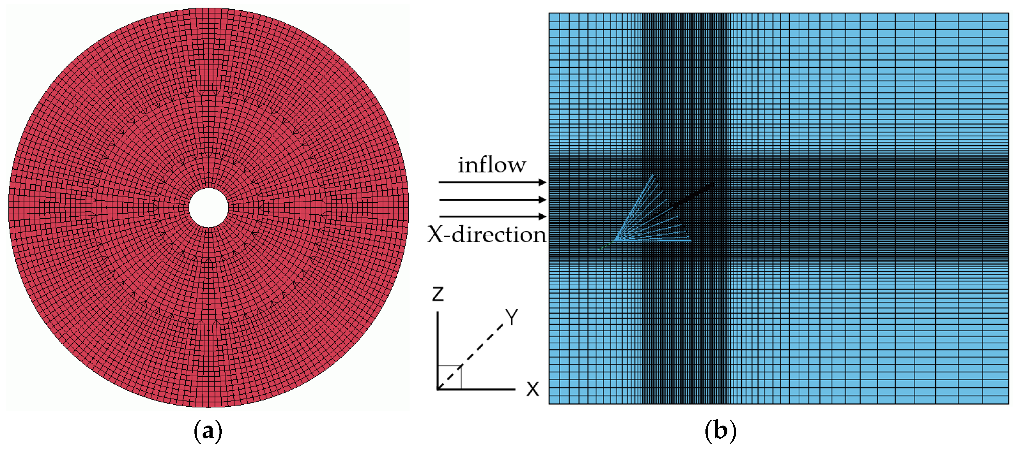
Figure 3 presents the finite element models for both the canopy and the flow field. With reference to the nominal diameter of the canopy, denoted as D0, the flow field domain is modeled using hexahedral elements, forming a rectangular cuboid with dimensions of 5D0 (spanwise, y-direction) × 5D0 (normal, z-direction) × 6D0 (streamwise, x-direction). Structural grids are interspersed within the flow field grids, and localized refinement is applied to the structural region of the high-altitude parachute canopy. A velocity inlet boundary condition is employed for the incoming flow. To prevent interference with the computational domain of the flow field, the remaining external boundaries are set as non-reflective boundaries. The specific parameters utilized in the model are detailed in Table 2.

3.2. Computational Case

This study investigates the effects of permeability variations on the structural response of the high-altitude wind-capturing umbrella set at a 30° attack angle, under two different canopy thicknesses. Based on the simplified Ergun formula provided in Equation (16), we investigate the influence of varying the viscosity coefficient a and inertia coefficient b on the canopy structure response. Increasing a and b reduces permeability, while decreasing a and b increases it. The six cases with a 30° attack angle are named Models A through F. The 0° attack angle case, called Model G, is used for mesh convergence testing and validation, as shown in Table 3. An initial flow velocity of 15 m/s is chosen for this study.

3.3. Measurement Criteria

Due to the limited number of suspension lines, the wrinkles in the canopy gores are relatively large. Therefore, this paper selects the canopy’s inner and outer radius as the measurement standards, with their sum representing the projected diameter. Subsequently, the vent radius was also measured. Given the presence of a severe collapsed state, the measurement standards adopted in this paper are illustrated in Figure 4. The projected diameter D is calculated using the following formula:
D = R 1 + R 2
where R1 is the outer radius, R2 is the inner radius.
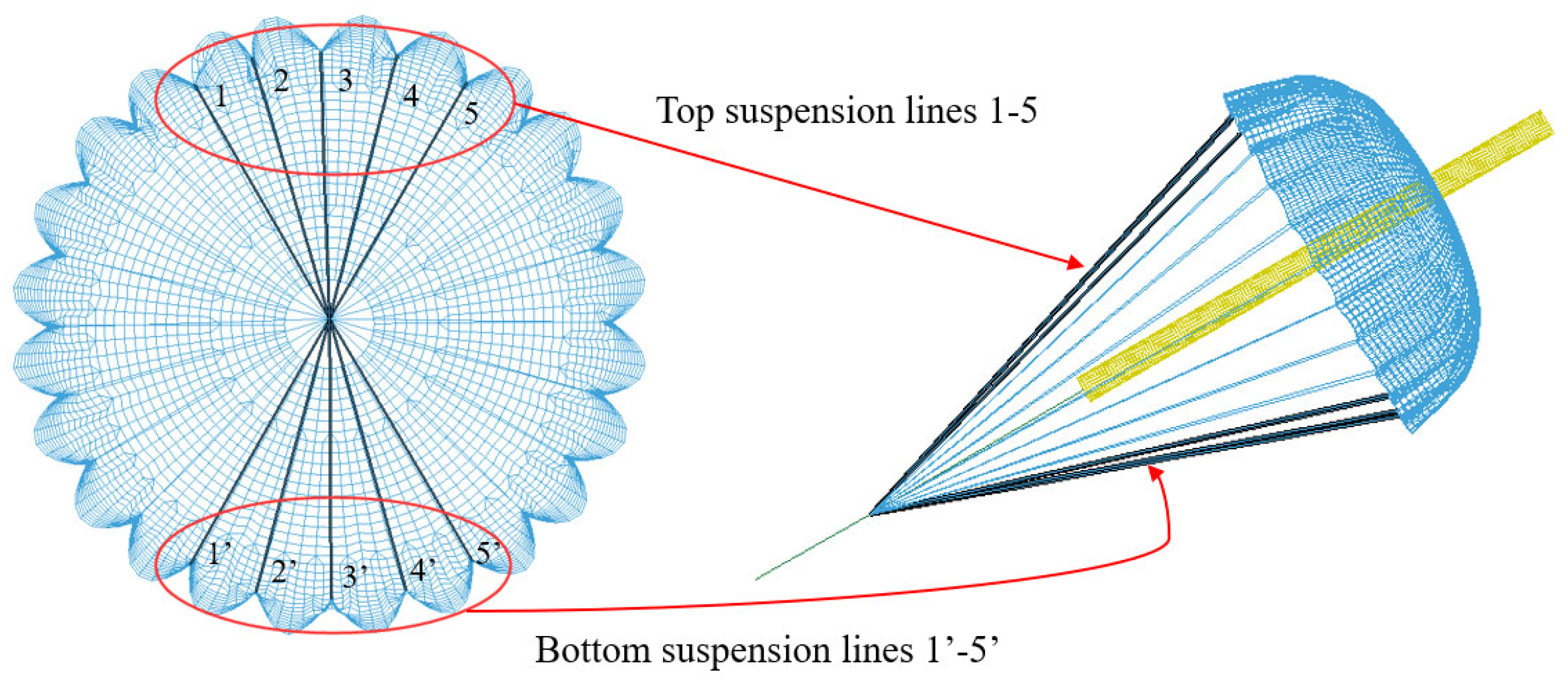
To compare the tensile forces of the top and bottom sets of suspension lines after the canopy stabilizes, we selected five top suspension lines. We numbered them as 1–5, along with their corresponding five bottom suspension lines numbered as 1′–5′. The loads on five suspension lines from both the top and bottom sections were measured individually. Subsequently, the mean loads of the top and bottom groups were calculated and compared, as illustrated in Figure 5.
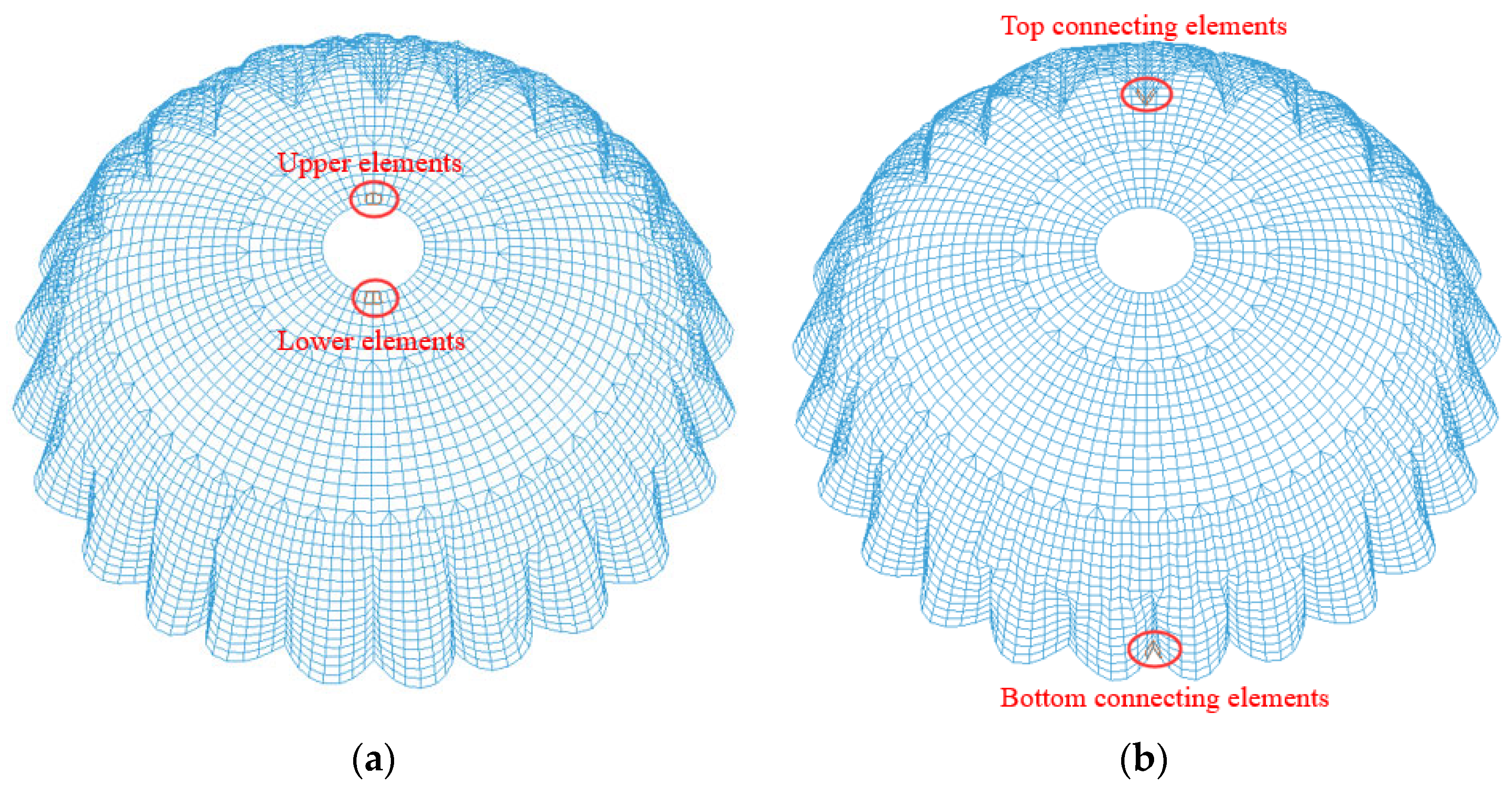
In Section 4.2, it will be shown that significant stress intensities are observed in the canopy elements at the suspension line-canopy connection points, as well as the vent elements. To quantify the stress magnitudes in the upper and lower sections of the stabilized canopy. For the vent, the mean stress values were calculated from elements located in the upper elements, and the same averaging procedure was applied to the lower section. Subsequently, a similar methodology was applied at each suspension line-canopy attachment point. Figure 6 shows the measurement elements.
To evaluate the magnitude of cable tension, the cable tension coefficient is defined as
C t = T 1 2 ρ V 2 S
where T is the cable tension force, ρ is the fluid density, V is the fluid velocity, and S is the nominal canopy area.

3.4. Mesh Convergence Test and Verification

This study investigates mesh convergence using a 0° angle of attack model. Four different fluid field mesh sizes were employed, with locally refined meshes in the overlapping region between the fluid field and canopy structure. The mesh density increased progressively from sparse to dense. As shown in Figure 7, the minimum mesh sizes in the locally refined regions were 300 mm, 200 mm, 120 mm, and 100 mm. The overall sum of fluid field grids ranged from 499,800 to 4,818,975. At 0° angle of attack, the cable tension coefficient aligns with the canopy drag coefficient. Therefore, in addition to grid convergence analysis, the validity of the model’s drag coefficient was also verified. The drag coefficient of canopy of the same type may vary slightly due to differences in canopy size, canopy gores, etc. Still, they all vary within a specific range. For a flat circular canopy, the range of its drag coefficient is 0.75–0.8 [37]. To better verify the rationality of the model, the median value of 0.775 is used as a benchmark for comparison with the results.
The comparison of the tension coefficient of the cable after the canopy is fully inflated is shown in Table 4. The drag coefficient tends to stabilize as the number of grids increases. The errors of Mesh B, C, and D are already minor, all within 10%, which meets the needs of engineering calculations. Although Mesh B has fewer minor errors, its stability when the canopy is filled is not as good as that of Mesh C and Mesh D. Mesh D has a longer calculation time. Based on a comprehensive consideration of calculation accuracy, efficiency, and canopy stability, this study ultimately selected a model with a minimum mesh size of 120 mm in the locally refined region and a total flow field mesh count of 2,729,712 to investigate the impact of permeability variations on canopy structural response at a 30° angle of attack for the high-altitude wind-catching canopy under two different canopy thicknesses.

4. Results and Discussion

Permeability significantly affects the wind-capturing performance of the High-altitude wind-capturing umbrella and has a greater impact on the canopy’s structural response. Therefore, this paper investigates the effect of permeability on the structural response of the High-altitude wind-capturing umbrella using the model listed in Table 3. This section first discusses the impact of permeability on canopy inflation, then analyzes the mechanical properties of the canopy.

4.1. Inflation Shape

Table 5 presents a comparison of the canopy morphology after stabilization for each operating condition, where Model A exhibits severe collapse, Models B and D show slight collapse, and Models C–F can be filled.
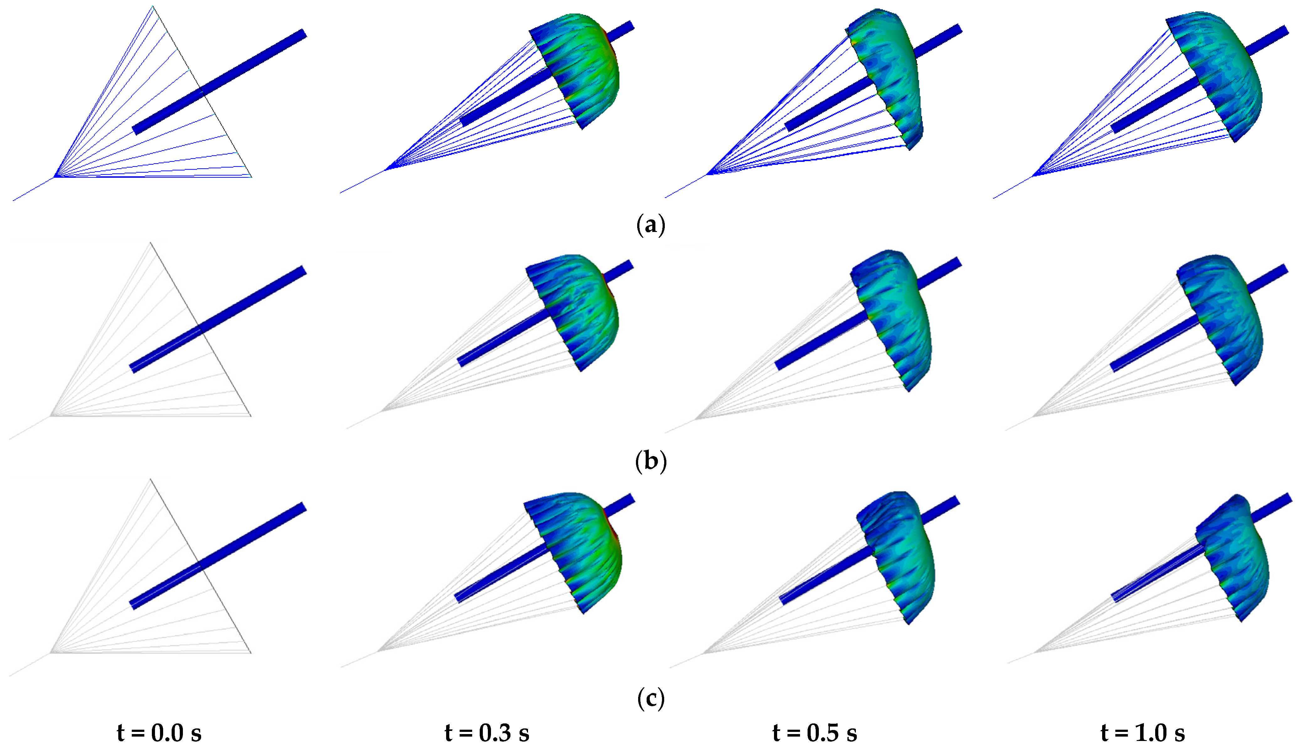
Figure 8 shows the inflation process of the high-altitude wind-capturing umbrella from 0.0 s to 1.0 s. In the initial stage of inflation (0.0–0.3 s), the inflation state of each Model is essentially the same. The canopy becomes bulb-shaped after the airflow reaches the vent. Subsequently, the airflow moves in the radial direction of the canopy, which causes the canopy to maintain its inflation. With the canopy undergoing inflation, the suspension lines progressively deploy, and the lower part of the canopy inflates faster than the upper part at 0.5 s, causing its radius to increase. The smaller the permeability, the greater the increase in the lower part of the radius. After the canopy’s lower part gradually fills up, then the upper part starts inflating, Models C–F which can be fully inflated become semi-circular after filling up, the upper part of the canopy of Model B and D is difficult to unfold fully, and the upper part of Model A is in the state of completely collapsed. It can be seen that the permeability has a greater impact on the stable shape of the High-altitude wind-capturing umbrella.
The smaller the viscosity and inertia coefficients (a and b), and the thinner the canopy, the higher the permeability, and the more difficult it is to inflate and unfold the upper part of the canopy. This is because lower canopy permeability allows less airflow to pass through its surface. As a result, more airflow flows back radially along the canopy cover, enabling the upper part to inflate. At this point, the pressure in front of the canopy remains stagnant, creating a high-pressure zone, which helps the canopy become more fully inflated.
The canopy is stabilized after 1.0 s, and its various structural responses have converged so that all subsequent data will be analyzed on the High-altitude wind-capturing umbrella state at 1.0 s.
The smaller the permeability of the canopy, the less airflow will pass through the canopy, and the fuller the canopy will be at this time. Therefore, we chose the ratio of projected to nominal diameter and the change in the radius of the vent of the canopy as the parameters to describe the inflation status of the canopy under each case. Figure 9 summarizes the measurement results according to the measurement criteria defined in Section 3.3.
Figure 9 shows that, at the same canopy thickness, the vent radius of the canopy increases as the air permeability decreases. Since the upper part of Model A is collapsed, as shown in Section 4.2, its vent is in the form of a water droplet. Hence, its vent radius is lower according to the measurement standard. Its projected diameter is also lower, indicating that the lower part is less inflated compared to the other models. For the models in the filled state, the difference in their vent radius is not significant, indicating that the effect of canopy air permeability on the canopy vent in the filled state is not essential. Figure 9b shows the variation in the ratio between the projected diameter and the nominal diameter, which increases at the same thickness as the permeability decreases with fuller filling. The projected diameters at 0.1 mm thickness of the canopy are all greater than 0.05 mm. However, the thickness of the canopy has a lesser effect on the inflation fullness. The difference between Model C and Model F is only 3.41% under the same viscosity coefficient (a) and inertia coefficient (b).

4.2. Stress Distribution

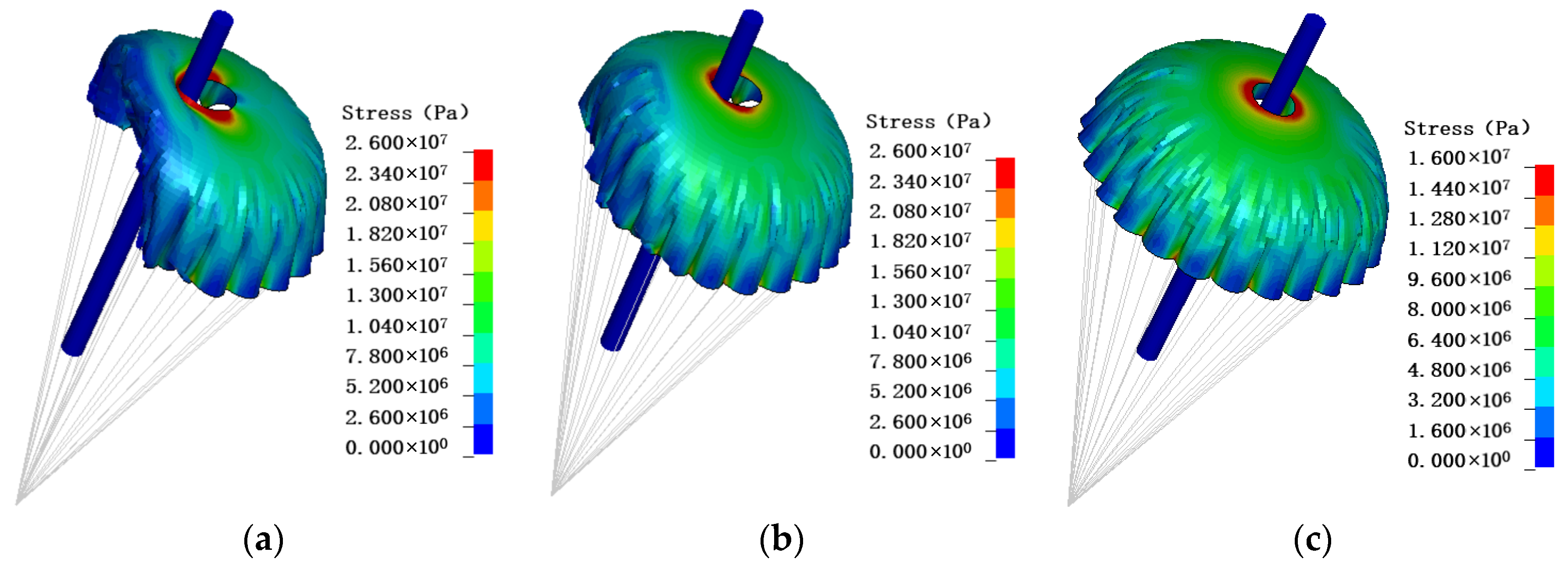
In the design of the canopy, it is necessary to consider its tear strength, so it is more important to analyze its surface stress. Figure 10 shows the stress distribution contour of the canopy under various inflation levels.
The larger value of the stress of the canopy is mainly concentrated in the vent and the connection between the canopy and the suspension lines. When the upper part of the canopy is seriously collapsed or slightly collapsed, the contact between the vent and the support of the canopy makes the stress concentrated and larger, and the distribution of the stress is in the form of a “swallow-tail shape”. In contrast, the stress on the windward side of the canopy at the collapsed place is lower. When the canopy is filled, the stress distribution is more uniform, and the airflow flows evenly from the vent.
To better understand the concentrated stresses in the canopy, stress changes in the upper and lower elements of the vent, as well as in the elements at the connection between the canopy and the suspension line, were measured according to the guidelines outlined in Section 3.3, as shown in Figure 11. In the filled state, the stress distributions of the upper and lower elements of the vent are basically equal. In contrast, in the collapsed state, the stress of the upper element is larger than that of the lower element, and the stress of the upper element in the filled state is smaller than that in the collapsed state. The viscosity coefficient a and inertial coefficient b of Model F and Model C are the same, and the larger the thickness of the canopy, the lower the stress in the vent. For the elements at the connection between the suspension line and the canopy, the stress at the top connection is greater than that at the bottom connection in the filled state, while the opposite is true in the collapsed state. That is because a lift force acts on the upper part of the canopy in the filled state, causing the canopy to tend to move upward. Consequently, the elemental stress at the top connection is greater than that at the bottom connection.
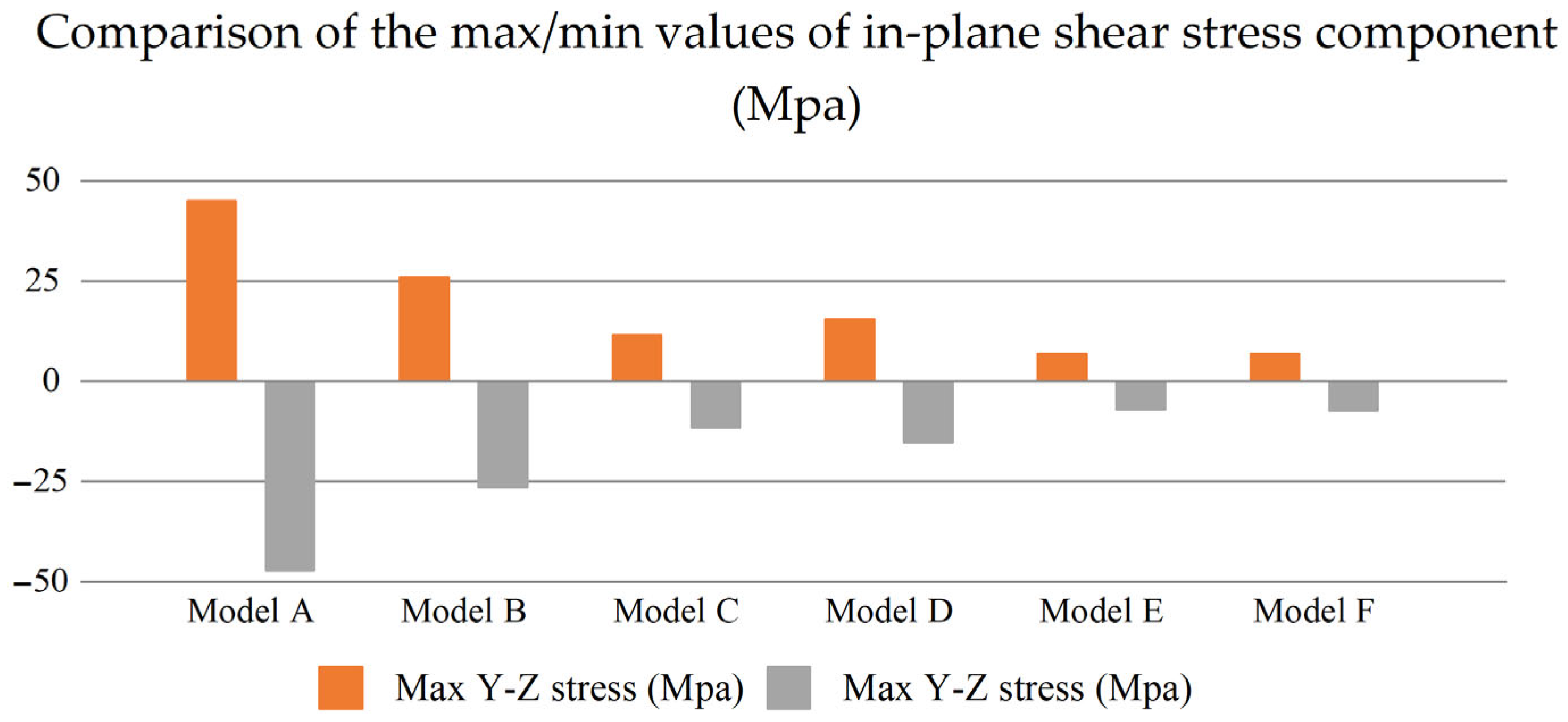
The maximum and minimum in-plane shear stresses of the canopy are shown in Figure 12. The plane is defined as shown in Figure 3b, and the normal plane of the flow direction is taken as the shear stress plane, which is the shear stress of the canopy in the Y-Z plane. These stresses are lower when the canopy is more fully inflated. Specifically, the maximum in-plane shear stress of Model F decreases by approximately 84.8%, and the minimum in-plane shear stress drops by 84.9% compared to Model A. To prevent damage to the canopy structure, reinforcements should be added at the vent and at the connection point between the canopy and the suspension lines.

4.3. Tension Coefficient and Axial Load in Suspension Lines

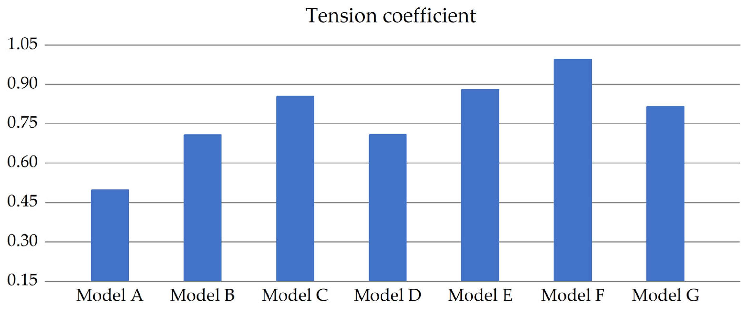
The tension coefficient determines the power generation efficiency of the umbrella ladder, and the tension coefficients for each case are shown in Figure 13. At the same canopy thickness, the tension coefficient rises as permeability decreases. When the canopy’s thickness doubles and both the viscosity coefficient, a, and the inertia coefficient, b, decrease by half, the tension coefficients are approximately the same, such as in Model B and Model D, and Model C and Model E. The tension coefficient of Model D with a 30° angle of attack exceeds that of Model G without an angle of attack because, when there is an angle of attack, the upper part of the canopy generates lift, and the lift and the wind captured by the umbrella cover work together on the cable, increasing its tension coefficient.
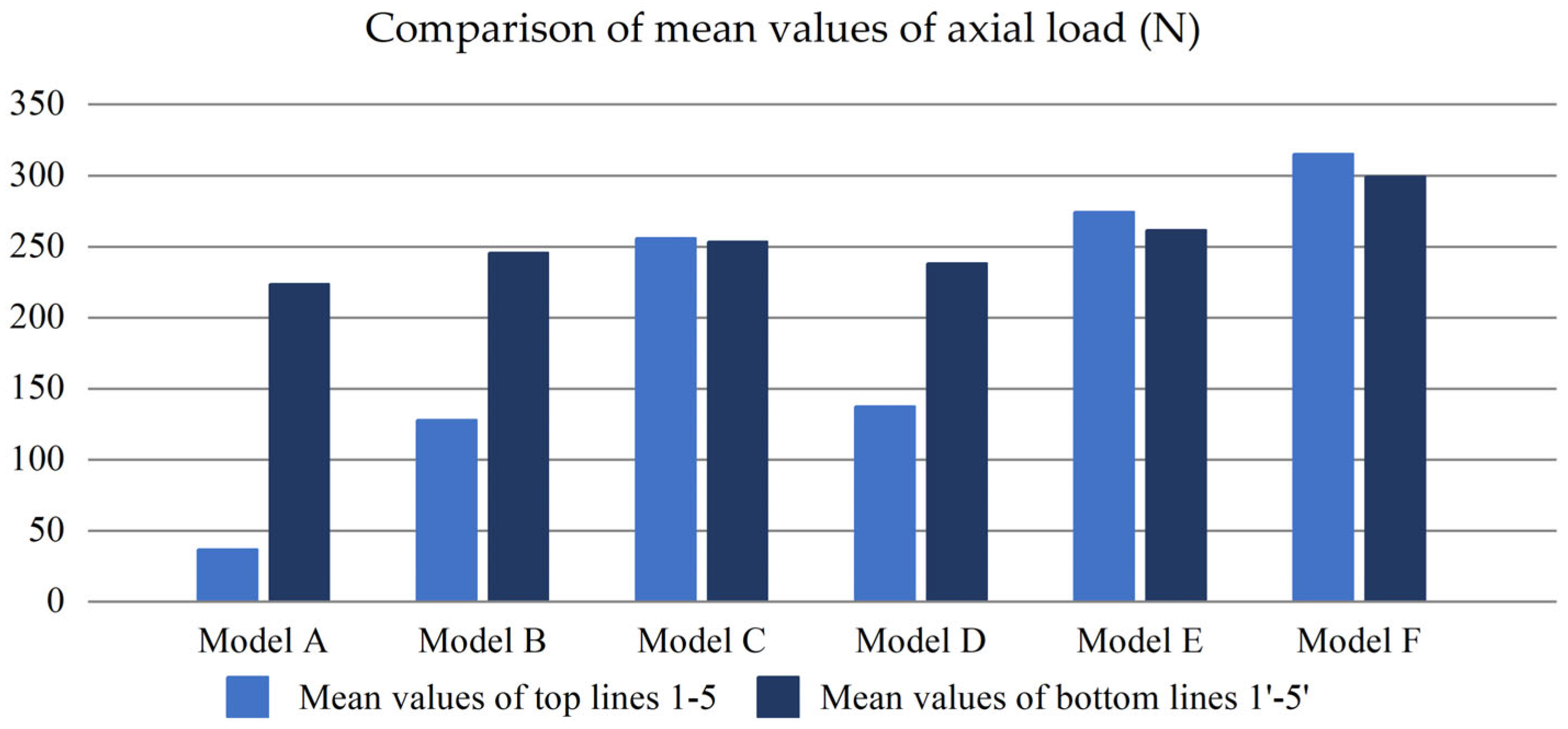
To better compare the tensile force generated by the top and bottom suspension lines, the top suspension lines are numbered 1–5. The bottom parachute lines numbered 1′–5′ were selected for axial load comparison. The average axial load of the two groups of parachute lines is shown in Figure 14. The results indicate that the axial load of the top and bottom suspension lines is essentially the same for the model in the filled state. However, the axial load of the top suspension line will be slightly larger than that of the bottom one, which is also caused by the lift force. The axial load of the upper suspension lines in the collapsed state is smaller than that of the lower ones, especially in the semi-collapsed state of Model A. The axial load of the lower suspension line of Model A is about 511% larger than that of the upper one, while that of Model B and Model D in the slightly collapsed state is 92.3% and 73.7%, respectively.

4.4. Flow Field Analysis

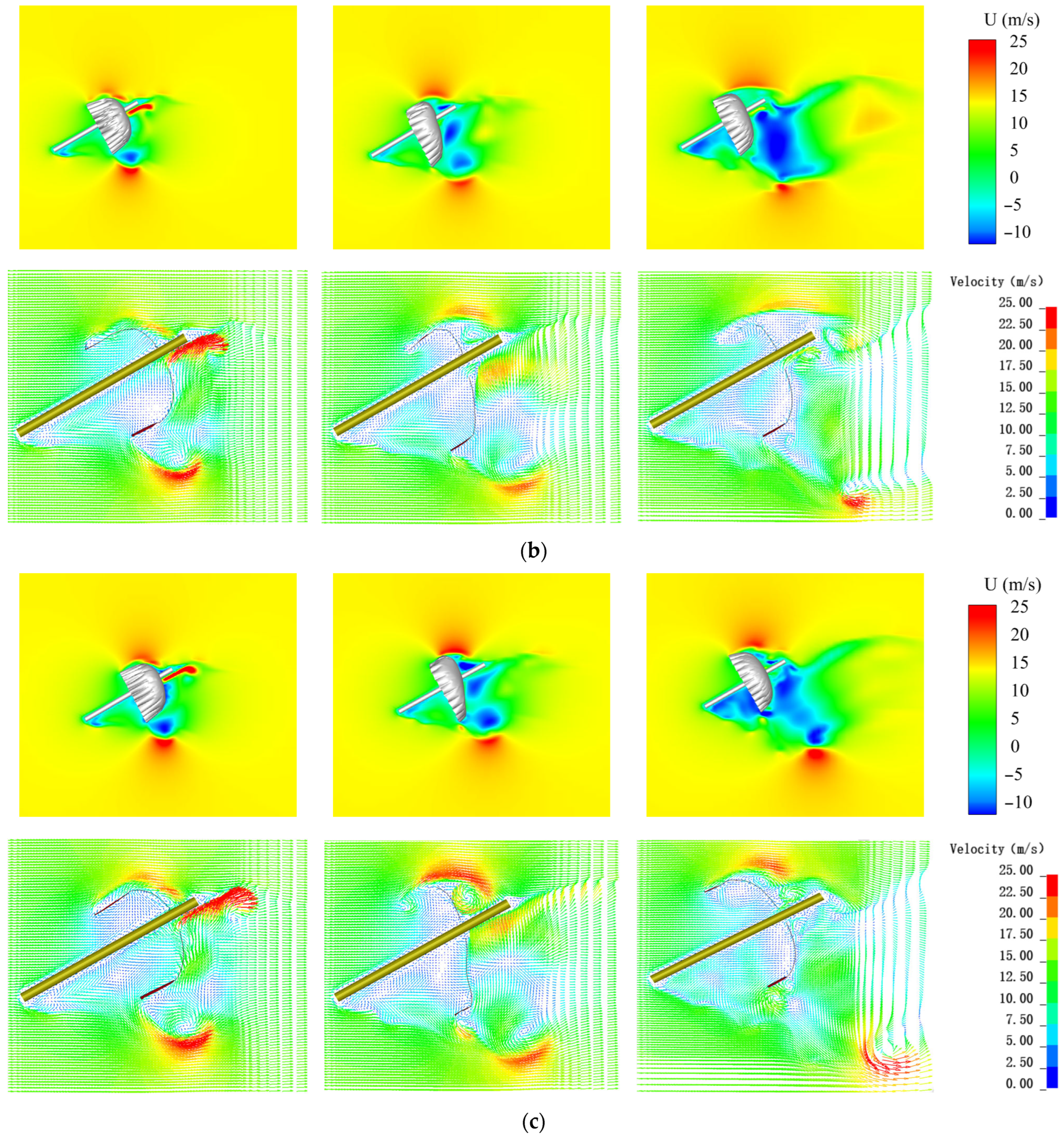
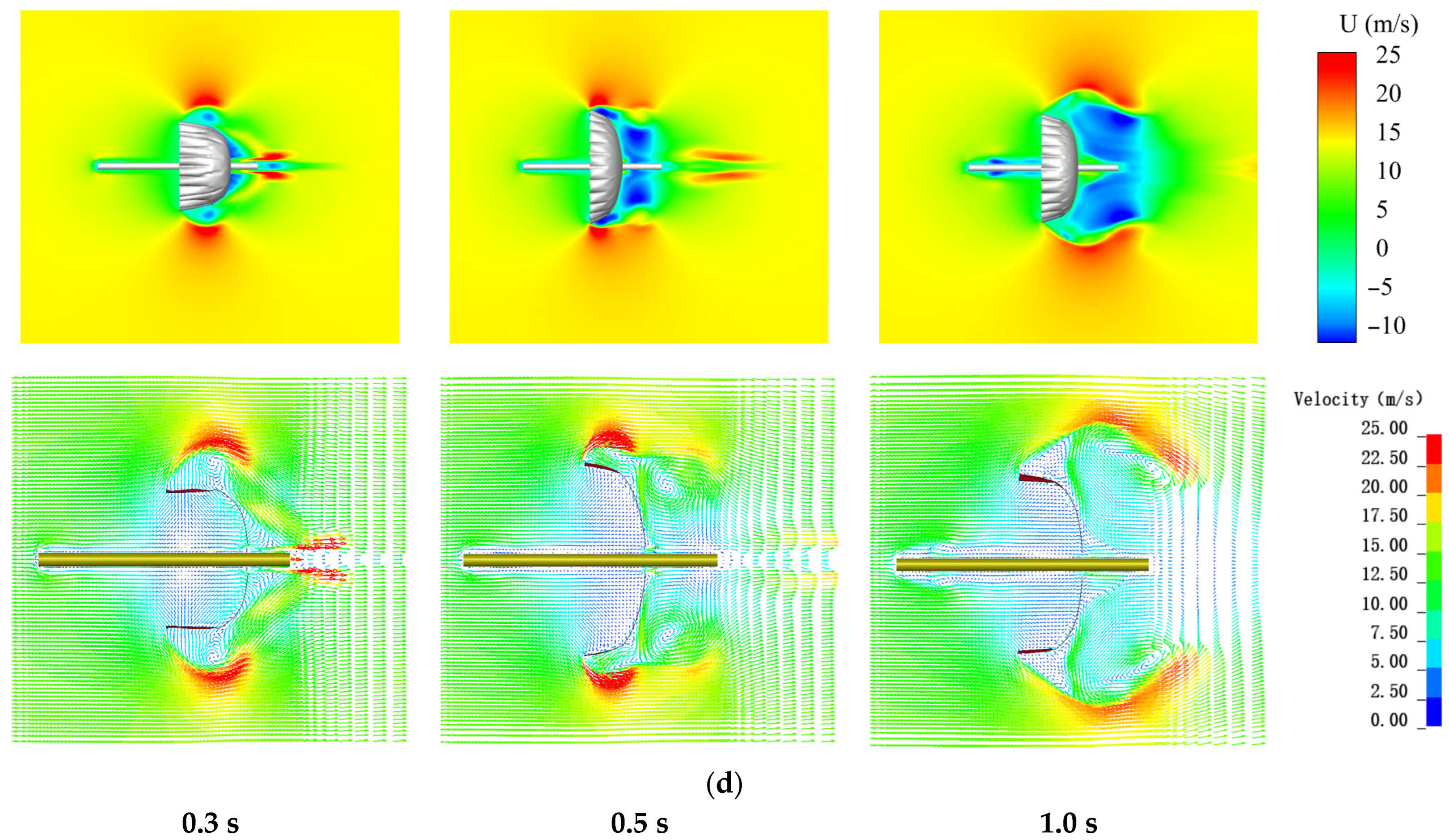
To better explain the lift generation mechanism mentioned in Section 4.2 and Section 4.3, we analyzed the flow field of the wind-capturing umbrella inflation process. Figure 15 shows that the flow field remains symmetrically distributed when there is no angle of attack. The deformation of the canopy and the flow field trails are also symmetrically distributed. However, when an angle of attack is present, the flow field distribution becomes asymmetric, leading to asymmetric deformation of the canopy and the formation of an asymmetric trailing vortical wake. During inflation, the asymmetric vortex behind the canopy gradually grows, and the flow field distribution turns non-uniform. With an angle of attack, the flow field at the lower outer edge of the canopy intensifies downstream. If multiple umbrella ladders are lined up side by side at this time, the flow field of the former set may interfere with that of the next.
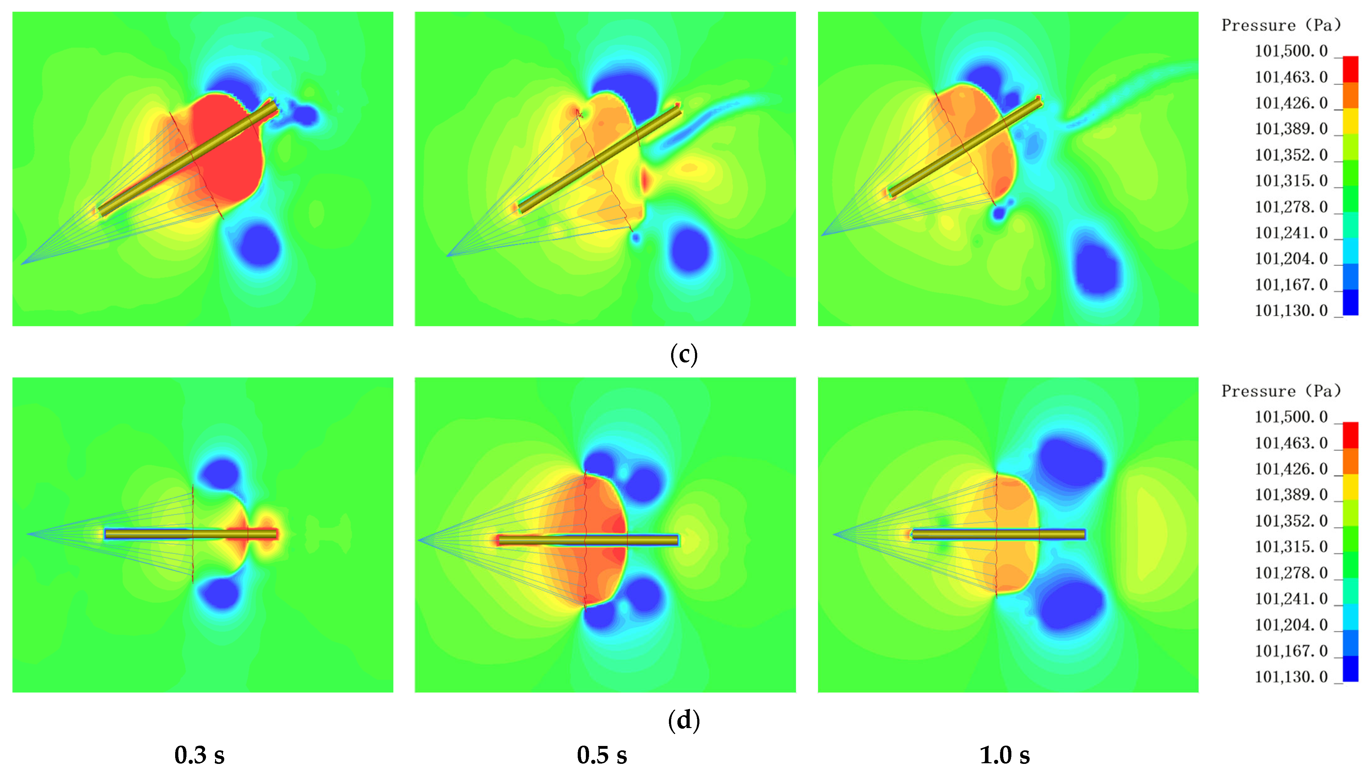
The flow field velocity in the upper part of the outer edge of the canopy is always higher. However, the velocity of the outer edge of the model in the collapsed state is lower than that in the filled state. Due to the acceleration of the outer edge, a low-pressure region forms, as shown in Figure 16. The collapsed model has higher permeability, resulting in lower velocity at the outer edge and a smaller pressure difference between the inner and outer parts of the canopy, which prevents it from filling. Conversely, the less permeable model exhibits a larger pressure difference, allowing airflow to unfold the canopy. The pressure difference causes the canopy in its filled state to generate lift. However, the wind force captured by the canopy is reduced compared to the case with no angle of attack. At this point, the combined force of lift and captured wind force is greater, leading to higher tension coefficients in Model C, Model E, and Model F than in Model G.
All the models initially show a “jet” at the vent. As the canopy continues to inflate, the support rod reduces the outflow of air through the vent, causing the “jet” to gradually weaken. The support rod limits the canopy’s angle of attack and also affects the flow field around it. Future research could explore the effects of support rod diameter and vent diameter on the tension coefficient.

5. Conclusions

This paper presents a fluid–structure interaction simulation of the high-altitude wind-capturing umbrella using the ALE method. The study examines how permeability influences the aerodynamic and structural response of the canopy under two different thicknesses. The main conclusions are as follows:
  • Under the same canopy thickness, the smaller the viscosity coefficient a and the inertia coefficient b are, the more permeable the canopy becomes, making it harder to inflate the upper part. Permeability has little impact on the radius of the vent and the diameter of the canopy projection.
  • The canopy is prone to stress concentration at the vent and at the connection between the canopy and the rope. The greater the permeability, the greater the stress generated by the contact with the support, and the smaller the permeability, the more uniform the stress distribution of the canopy. The max/min in-plane shear stress of the Model F with the smallest permeability is about 85% lower than the Model A with the most significant permeability.
  • At the same canopy thickness, the tensile coefficient increases as canopy thickness increases, and halving the canopy’s thickness results in a tensile coefficient similar to doubling the coefficients of viscosity a and inertia b. The axial load on the top suspension line is slightly higher than that on the bottom line in the filled state, with a difference of up to 92.3% during slight collapse. Additionally, this difference becomes much more significant during severe collapse.
  • The fluid field is always asymmetric when there is an angle of attack, and the acceleration zone at the outer edge of the lower part of the canopy affects the downstream flow field. The pressure difference between the inside and outside of the canopy causes it to generate a lift force, which increases the tension coefficient with angle of attack compared to the same conditions without an angle of attack.
In summary, permeability significantly affects the structural response of a high-altitude wind-capturing umbrella with an angle of attack. When designing the canopy, permeability should be minimized as much as possible while maintaining a certain canopy mass and stability to enhance wind energy conversion efficiency. The results of this paper can be used to guide the design of a high-altitude wind-capturing system of the same size at wind speeds of 15 m/s. For other canopy sizes, the tensile coefficient remains applicable within the Reynolds number range of 1.5 × 10⁵ to 1.3 × 10⁷. The stress results of canopies vary depending on their size and wind speed, and the stress results obtained in this paper are applicable for the qualitative analysis of the variation trends. Future research will focus on quantitatively comparing experimental and numerical simulation results, offering valuable guidance for designing and optimizing high-altitude wind-capturing umbrellas in umbrella–ladder-type Ground-Gen high-altitude wind power generation technology.

Author Contributions

Conceptualization, Y.W.; methodology, Y.W. and J.J.; numerical simulation, J.J.; formal analysis, J.J. and J.W.; data curation, J.J. and J.W.; writing—original draft preparation, J.J.; writing—review and editing, Y.W., C.C. and T.W.; supervision, Y.W. and C.C.; project administration, C.C.; funding acquisition, Y.W. and C.C. All authors have read and agreed to the published version of the manuscript.

Funding

This research was funded by the National Key R&D Program of China (No. 2023YFB4203401) and the State Key Laboratory of Mechanics and Control for Aerospace Structures (MCAS-I-0235G01). This work is also partially supported by High Performance Computing Platform of Nanjing University of Aeronautics and Astronautics.

Institutional Review Board Statement

Not applicable.

Informed Consent Statement

Not applicable.

Data Availability Statement

The data presented in this study are available on request from the corresponding author.

Conflicts of Interest

The authors declare no conflicts of interest.

References

  1. Msigwa, G.; Ighalo, J.; Yap, P. Considerations on environmental, economic, and energy impacts of wind energy generation: Projections towards sustainability initiatives. Sci. Total Environ. 2022, 849, 157755. [Google Scholar] [CrossRef]
  2. Tleubergenova, A.; Tanasheva, N.; Shaimerdenova, K.; Kassymov, S.; Bakhtybekova, A.; Shuyushbayeva, N.; Uzbergenova, S.; Ranova, G. Mathematical modeling of the aerodynamic coefficients of a sail blade. Adv. Aerodyn. 2023, 5, 14. [Google Scholar] [CrossRef]
  3. Caduff, M.; Huijbregts, M.; Althaus, H.; Koehler, A.; Hellweg, S. Wind power electricity: The bigger the turbine, the greener the electricity? Environ. Sci. Technol. 2012, 46, 4725–4733. [Google Scholar] [CrossRef]
  4. Khan, Z.; Rehan, M. Harnessing airborne wind energy: Prospects and challenges. J. Control Autom. Electr. Syst. 2016, 27, 728–740. [Google Scholar] [CrossRef]
  5. Malz, E.; Hedenus, F.; Göransson, L.; Verendel, V.; Gros, S. Drag-mode airborne wind energy vs. wind turbines: An analysis of power production, variability and geography. Energy 2020, 193, 116765. [Google Scholar] [CrossRef]
  6. Weliwaththage, S.; Yildirim, M.; Aksac, G.; Ulku, M. Airborne Wind Energy Technology. J. Res. Technol. Eng. 2021, 2, 22–29. [Google Scholar]
  7. Malz, E.; Walter, V.; Göransson, L.; Gros, S. The value of airborne wind energy to the electricity system. Wind Energy 2022, 25, 281–299. [Google Scholar] [CrossRef]
  8. Loyd, M. Crosswind kite power. J. Energy 1980, 4, 106–111. [Google Scholar] [CrossRef]
  9. Fagiano, L.; Milanese, M. Airborne wind energy: An overview. In Proceedings of the American Control Conference, Montreal, QC, Canada, 27–29 June 2012. [Google Scholar]
  10. Fagiano, L.; Quack, M.; Bauer, F.; Carnel, L.; Oland, E. Autonomous airborne wind energy systems: Accomplishments and challenges. Annu. Rev. Control Robot. Auton. Syst. 2022, 5, 603–631. [Google Scholar] [CrossRef]
  11. Cherubini, A.; Papini, A.; Vertechy, R.; Fontana, M. Airborne Wind Energy Systems: A review of the technologies. Renew. Sustain. Energy Rev. 2015, 51, 1461–1476. [Google Scholar] [CrossRef]
  12. Canale, M.; Fagiano, L.; Milanese, M.; Ippolito, M. KiteGen project: Control as key technology for a quantum leap in wind energy generators. In Proceedings of the American Control Conference, New York, NY, USA, 9–13 July 2007. [Google Scholar]
  13. Lansdorp, B.; Williams, P. The laddermill-innovative wind energy from high altitudes in holland and Australia. In Proceedings of the Global Windpower, Adelaide, Australia, 18–21 September 2006. [Google Scholar]
  14. Vermillion, C.; Cobb, M.; Fagiano, L.; Leuthold, R.; Diehl, M.; Smith, R.; Wood, T.; Rapp, S.; Schmehl, R.; Olinger, D.; et al. Electricity in the air: Insights from two decades of advanced control research and experimental flight testing of airborne wind energy systems. Annu. Rev. Control 2021, 52, 330–357. [Google Scholar] [CrossRef]
  15. Vermillion, C.; Grunnagle, T.; Kolmanovsky, I. Modeling and control design for a proto-type lighter-than-air wind energy system. In Proceedings of the American Control Conference, Montreal, QC, Canada, 27–29 June 2012. [Google Scholar]
  16. Sola, P.; McDonald, A.; Oterkus, E. A lightweight approach for airborne wind turbine drivetrains. In Proceedings of the European Wind Energy Association, Paris, France, 17–20 November 2015. [Google Scholar]
  17. Luo, B.; Ren, Z.; Liu, H. Analysis of Current Status and Prospects of Parachute-Based Airborne Wind Energy Technology. Electr. Power Constr. 2025, 46, 45–53. [Google Scholar]
  18. Li, J. Study on the Electromechanical Coupling Dynamics Modeling and Dynamic Characteristics of Ground Transmission Systems in High-Altitude Wind Power. Master’s Thesis, Chongqing Jiaotong University, Chongqing, China, 1 June 2024. [Google Scholar]
  19. Luo, B.; Hu, J.; Yang, Y.; Ren, Z.; He, Y. Modeling and stable operation control method for airborne wind energy system considering longitudinal disturbance stability. South Energy Constr. 2025, 12, 1–11. [Google Scholar]
  20. Zhang, Y.; Pu, T.; Jia, H.; Wu, S.; Zhou, C. Extension of a sharp-interface immersed-boundary method for simulating parachute inflation. Adv. Aerodyn. 2024, 6, 3. [Google Scholar] [CrossRef]
  21. Taguchi, M.; Semba, N.; Mori, K. Effects of flexibility and gas permeability of fabric to supersonic performance of flexible parachute. In Proceedings of the 23rd AIAA Aerodynamic Decelerator Systems Technology Conference, Daytona Beach, FL, USA, 30 March–2 April 2015. [Google Scholar]
  22. Xu, X.; Jia, H.; Chen, Y. Influence mechanism of fabric permeability of canopy on aerodynamics of Mars parachute. Acta Areonaut. Astronaut. Sin. 2022, 43, 307–324. [Google Scholar]
  23. Yang, X.; Yu, L.; Nie, S.; Zhang, S. Aerodynamic performance of the supersonic parachute with material permeability. J. Ind. Text. 2021, 50, 812–829. [Google Scholar] [CrossRef]
  24. Yu, L.; Ming, X.; Chen, L. Experimental investigation on the flow-field of different vent canopy. Acta Aerodyn. Sin. 2008, 26, 19–25. [Google Scholar]
  25. Zeng, Y.; Wang, Y.; Yuan, H. A stable and efficient semi-implicit coupling method for fluid-structure interaction problems with immersed boundaries in a hybrid CPU-GPU framework. J. Comput. Phys. 2025, 534, 114026. [Google Scholar] [CrossRef]
  26. Guan, L.; Yu, G.; He, X. Inflation process of radially closed parachute. Phys. Fluids 2025, 37, 025109. [Google Scholar] [CrossRef]
  27. Huang, Y.; Wu, S.; Zhang, Y. Effect of different steering approaches on gliding performance of cruciform parachute. Manned Spacefl. 2024, 30, 52–59. [Google Scholar]
  28. Huang, Y.; Wu, S.; Wang, Y. Numerical and experimental investigation of the steering performance of a ringsail parachute. J. Northwest. Polytech. Univ. 2024, 42, 1021–1029. [Google Scholar] [CrossRef]
  29. Cao, H.; Huang, L.; Li, X. Research on control force of parafoil based on fluid structure interaction method. Acta Aeronaut. Astronaut. Sin. 2025, 46, 148–158. [Google Scholar]
  30. Hou, X.; Hu, J.; Yu, Y. Numerical Study of Aerodynamic Characteristics of No-Swinging and Free-to-Swing Cross Parachute. AIAA J. 2023, 61, 5018–5031. [Google Scholar] [CrossRef]
  31. Li, K.; Wang, Z.; Ma, Y.; Wang, Y.; Li, H. Research on the inflation process of underwater parachute by numerical simulation and model test. Ocean Eng. 2024, 293, 116554. [Google Scholar] [CrossRef]
  32. Souli, M.; Ouahsine, A.; Lewin, L. ALE formulation for fluid–structure interaction problems. Comput. Methods Appl. Mech. Eng. 2000, 190, 659–675. [Google Scholar] [CrossRef]
  33. Lee, H.; Xu, S. Fully discrete error estimation for a quasi-Newtonian fluid–structure interaction problem. Comput. Math. Appl. 2016, 71, 2373–2388. [Google Scholar] [CrossRef]
  34. Yu, L.; Cheng, H.; Zhan, Y.; Li, S. Study of parachute inflation process using fluid–structure interaction method. Chin. J. Aeronaut. 2014, 27, 272–279. [Google Scholar] [CrossRef]
  35. Ergun, S. Fluid flow through packed columns. Chem. Eng. Prog. 1952, 48, 89. [Google Scholar]
  36. Nie, S.; Yu, L.; Li, Y.; Sun, Z.; Qiu, B. Influence of fabric permeability on breathing phenomenon of supersonic parachute. J. Ind. Text. 2023, 53, 15280837231171733. [Google Scholar] [CrossRef]
  37. Li, Z. Wind Tunnel Special Tests Technique; Aviation Industry Press: Beijing, China, 2010; p. 493. [Google Scholar]
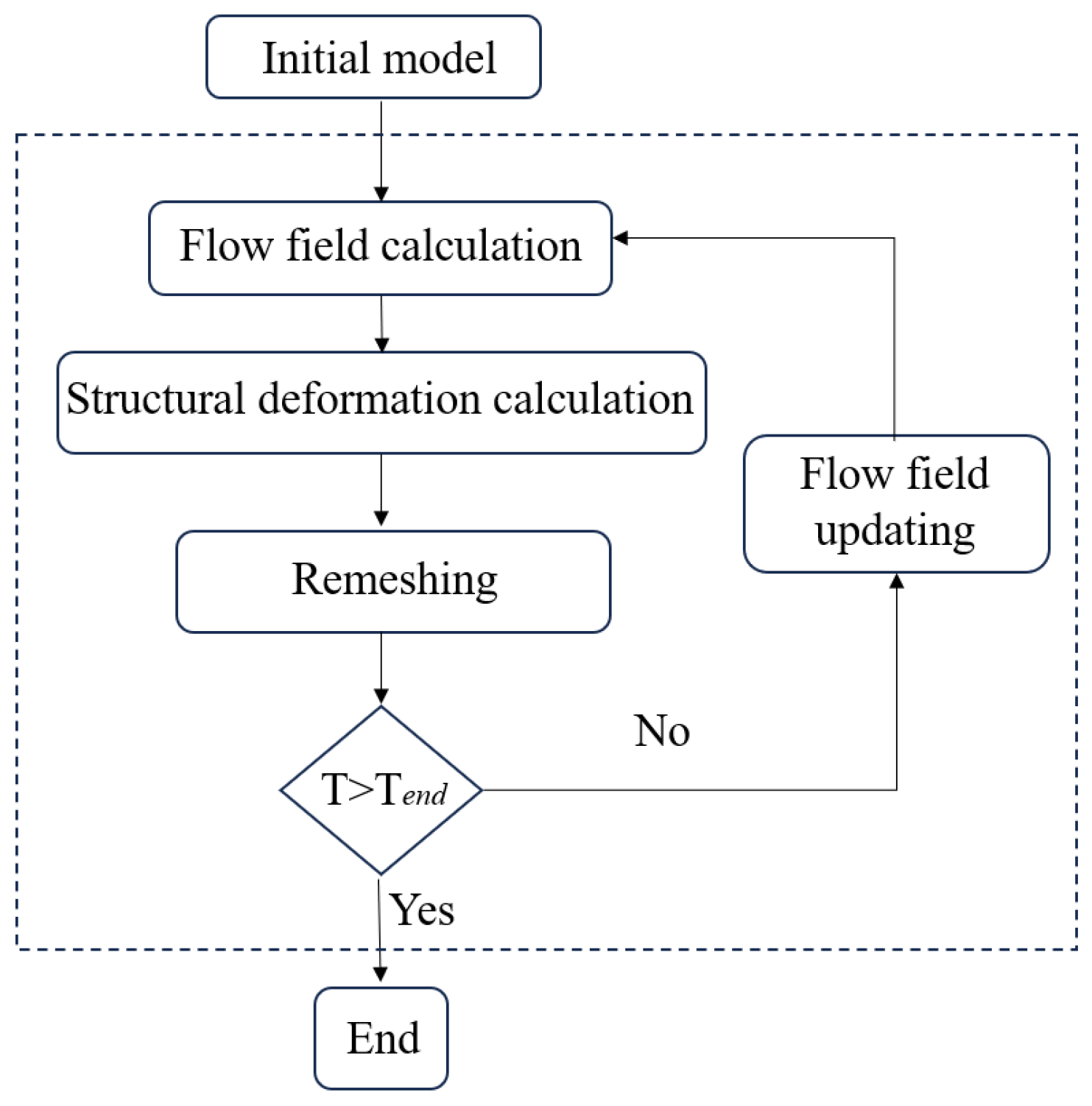
Figure 1. Fluid–structure interaction process.
Applsci 15 12161 g001
Figure 2. Geometric models. (a) High-altitude wind-capturing umbrella. (b) Flow field.
Applsci 15 12161 g002
Figure 3. Finite element model. (a) Canopy mesh. (b) Fluid field mesh.
Applsci 15 12161 g003
Figure 4. Measurement criteria for the canopy outer radius R1, inner radius R2, and the vent radius r. (a) Fully inflated. (b) Severely collapsed.
Applsci 15 12161 g004
Figure 5. The number of top and bottom suspension lines for measurement.
Applsci 15 12161 g005
Figure 6. Measurement criteria for canopy element stress. (a) Upper and lower elements around the vent. (b) The connecting elements between the canopy and the suspension line are at the top and the bottom.
Applsci 15 12161 g006
Figure 7. Locally refined region in fluid field mesh. (a) mesh A. (b) mesh B. (c) mesh C. (d) mesh D.
Applsci 15 12161 g007
Figure 8. The canopy shapes change during inflation. (a) Fully inflated. (b) Slightly collapsed. (c) Severely collapsed.
Applsci 15 12161 g008
Figure 9. Effect of permeability on canopy inflation. (a) Radius of vent. (b) The ratio of projected to nominal diameter.
Applsci 15 12161 g009
Figure 10. Stress contours on the canopy surface. (a) Severely collapsed. (b) Slightly collapsed. (c) Fully inflated.
Applsci 15 12161 g010
Figure 11. Stress of elements at the stress concentration. (a) Stress of elements around the vent. (b) Stress of the connecting elements.
Applsci 15 12161 g011
Figure 12. In-plane shear stress components of the canopy.
Applsci 15 12161 g012
Figure 13. Tension coefficient.
Applsci 15 12161 g013
Figure 14. Axial load in the top and bottom suspension lines.
Applsci 15 12161 g014
Figure 15. Velocity Contours of the Flow Field. (a) Severely collapsed. (b) Slightly collapsed. (c) Fully inflated. (d) Model G.
Applsci 15 12161 g015aApplsci 15 12161 g015bApplsci 15 12161 g015c
Figure 16. Pressure Contours of the Flow Field. (a) Severely collapsed. (b) Slightly collapsed. (c) Fully inflated. (d) Model G.
Applsci 15 12161 g016aApplsci 15 12161 g016b
Table 1. Geometric parameters of the wind-capturing umbrella system.
ParameterValue
Canopy nominal diameter D0 (m)8.4
Suspension line length (m)8.4
Vent diameter (m)0.84
Support rod diameter (m)0.42
Support rod length (m)8.35
Table 2. The element parameter.
ParameterCanopySuspension LineFluid
Type of elementsShellBeamSolid
Density (kg·m−3)533.7711541.225
Young’s modulus (Pa)4.31 × 1087.3 × 1010-
Poisson’s ratio0.14--
MaterialsFabricCableNull
Number of elements470410082,729,712
Table 3. Parameters for different models.
ModelsAttack AngleThickness
(m)
Viscosity Coefficient (a)
(kg/(m3·s))
Inertial Coefficient (b)
(kg·m−4)
A30°5 × 10−58 × 1052.4 × 105
B1.6 × 1064.8 × 105
C3.2 × 1069.6 × 105
D30°1 × 10−48 × 1052.4 × 105
E1.6 × 1064.8 × 105
F3.2 × 1069.6 × 105
G1 × 10−41.6 × 1064.8 × 105
Table 4. Fluid field mesh convergence test.
MeshMinimum Mesh Size
(mm)
Simulation Time
(hour)
Number of Mesh ElementsDrag CoefficientError
A300 × 300 × 3002499,8000.53531%
B200 × 200 × 2004.11,205,9360.7542.7%
C120 × 120 × 12092,729,7120.8165.3%
D100 × 100 × 10067.54,818,9750.7922.2%
Table 5. Shapes of the canopy after inflation stabilization.
ModelShape
ASeverely collapsed
BSlightly collapsed
CFully inflated
DSlightly collapsed
EFully inflated
FFully inflated
Disclaimer/Publisher’s Note: The statements, opinions and data contained in all publications are solely those of the individual author(s) and contributor(s) and not of MDPI and/or the editor(s). MDPI and/or the editor(s) disclaim responsibility for any injury to people or property resulting from any ideas, methods, instructions or products referred to in the content.