Improved Super-Resolution Reconstruction Algorithm Based on SRGAN

Abstract

To improve the performance of image super-resolution reconstruction, this paper optimizes the classical SRGAN model architecture. The original SRResNet is replaced with the EDSR network as the generator, which effectively enhances the ability to restore image details. To address the issue of insufficient multi-scale feature extraction in SRGAN during image reconstruction, an LSK attention mechanism is introduced into the generator. By fusing features from different receptive fields through parallel multi-scale convolution kernels, the model improves its ability to capture key details. To mitigate the instability and overfitting problems in the discriminator training, the Mish activation function is used instead of LeakyReLU to improve gradient flow, and a Dropout layer is introduced to enhance the discriminator’s generalization ability, preventing overfitting to the generator. Additionally, a staged training strategy is employed during adversarial training. Experimental results show that the improved model effectively enhances image reconstruction quality while maintaining low complexity. The generated results exhibit clearer details and more natural visual effects. On the public datasets Set5, Set14, and BSD100, compared to the original SRGAN, the PSNR and SSIM metrics improved by 13.4% and 5.9%, 9.9% and 6.0%, and 6.8% and 5.8%, respectively, significantly enhancing the reconstruction of super-resolution images, achieving more refined and realistic image quality improvement. The model also demonstrates stronger generalization ability on complex cross-domain data, such as remote sensing images and medical images. The improved model achieves higher-quality image reconstruction and more natural visual effects while maintaining moderate computational overhead, validating the effectiveness of the proposed improvements.

1. Introduction

Super-Resolution Reconstruction (SRR) is a technique that converts low-resolution images into high-resolution images through algorithms, aiming to restore high-frequency details in images and make them clearer and more realistic. In recent years, with the rapid development of deep learning, SRR has made significant progress and has been widely applied in fields such as medical imaging [1], facial recognition, security surveillance, video processing, and satellite remote sensing, achieving good results. Researchers have continuously explored optimization methods to improve image reconstruction quality while reducing computational overhead, aiming to meet the dual demands of speed and accuracy in practical applications. Various network architectures have been proposed for this purpose, including traditional interpolation methods (such as bilinear interpolation and bicubic interpolation), sparse representation-based reconstruction methods, and deep convolutional neural network (CNN)-based methods [2,3]. Dong et al. [4] proposed the SRCNN (Super-Resolution Convolutional Neural Network), which performs super-resolution reconstruction of images through an end-to-end training approach. By leveraging the characteristics of deep convolutional neural networks, SRCNN significantly improved image quality. However, due to its limited network depth, it performed poorly in handling complex textures and high-frequency details. Later, Kim et al. [5] proposed VDSR (Very Deep Super-Resolution), which increased network depth to further improve reconstruction results. However, this also led to higher computational costs and training difficulty. Shi et al. [6] developed the ESPCN (Efficient Sub-Pixel Convolutional Neural Network), which introduced sub-pixel convolution to improve upscaling efficiency. However, in some cases, the reconstructed details still lacked precision [7].

Although these studies have improved SRR performance to varying degrees, they still have limitations, particularly when handling high-frequency details and complex image structures, where blurring and information loss are common issues. With the introduction of Generative Adversarial Networks (GANs), especially the advent of Super-Resolution Generative Adversarial Networks (SRGANs), these issues have been effectively addressed. SRGAN generates high-resolution images through adversarial learning between the generator and the discriminator. The generator is responsible for reconstructing low-resolution images into high-resolution ones, while the discriminator distinguishes between generated images and real high-resolution images [8]. This adversarial training mechanism enables SRGAN to effectively capture details and complex structures in images, greatly enhancing the realism and visual quality of the reconstructed images [9]. Compared to traditional interpolation methods and other deep learning approaches, SRGAN excels in quantitative metrics like PSNR and SSIM, and it also achieves significant improvements in visual effects. However, the original SRGAN model suffers from high parameter counts, slow convergence, and potentially lacks diversity in the generated image details, with training instability being another issue [10].

Currently, there are three key gaps in SRGAN research: First, SRGAN model exhibits elevated computational complexity and has a clear deficiency in multi-scale feature extraction [11]. Its fixed-size convolution kernels (usually 3 × 3) are inadequate for capturing both local details and global contextual information simultaneously, leading to poor reconstruction of complex textures such as hair or repetitive patterns [12]. Second, overfitting of the discriminator in adversarial training is a common problem, and existing methods lack effective regularization strategies (e.g., structural Dropout or feature perturbation). When training data is limited, the discriminator converges too early, suppressing the optimization of the generator [13]. Finally, most existing methods are evaluated primarily on natural images (e.g., animals, landscapes), with a lack of systematic validation in cross-domain scenarios (e.g., medical imaging, remote sensing images), making it difficult to demonstrate their generalization ability.

This paper proposes a series of innovative improvements to address the redundancy in the network structure, low computational efficiency, insufficient multi-scale feature extraction, and instability in the training process of the traditional SRGAN model in image super-resolution reconstruction tasks. In the generator, we replace the original SRResNet structure with the EDSR network [14], which significantly improves computational efficiency by streamlining the network architecture. Meanwhile, the BN layers are removed to eliminate feature distribution shift, effectively reducing artifacts in the generated images. To enhance the network’s ability to extract multi-scale features, we incorporate the LSK attention mechanism [15] with dynamic multi-scale properties. The core innovation of this mechanism lies in transferring the concept of large kernel attention from remote sensing image processing to the super-resolution domain [16]. Unlike traditional fixed-size convolution kernels, this module uses dynamic weight allocation through parallel 3 × 3, 5 × 5, and 7 × 7 convolution kernels, enabling adaptive perception of both local textures and global structures, thereby capturing both local details and global contextual information. For discriminator optimization, we replace the traditional LeakyReLU [17] activation function with the Mish [18] activation function, which improves gradient flow stability due to its continuous differentiable characteristics. Additionally, we introduce a Dropout layer [19] to prevent overfitting of the discriminator, effectively enhancing the model’s generalization ability [20]. In terms of training strategy optimization, we propose a staged adversarial training strategy to address the overfitting of the discriminator and the imbalance of training dynamics. This strategy is based on the progressive equilibrium principle of asymmetric games [21]: (1) In the pre-training stage, we prioritize strengthening the discriminator’s feature discrimination ability, fixing the generator’s parameters to help the discriminator quickly establish an effective gradient signal space; (2) In the adversarial balancing stage, we introduce a dynamic learning rate adjustment mechanism, periodically decaying optimizer parameters to achieve synchronized evolution of the generator and discriminator.

Experimental results show that the improved model significantly enhances image reconstruction quality while maintaining low computational complexity. The generated super-resolution images exhibit clearer edge details and more natural visual effects, while the training process shows better stability. These improvements make the model more practical for real-world applications.

2. SRGAN Algorithm Structure

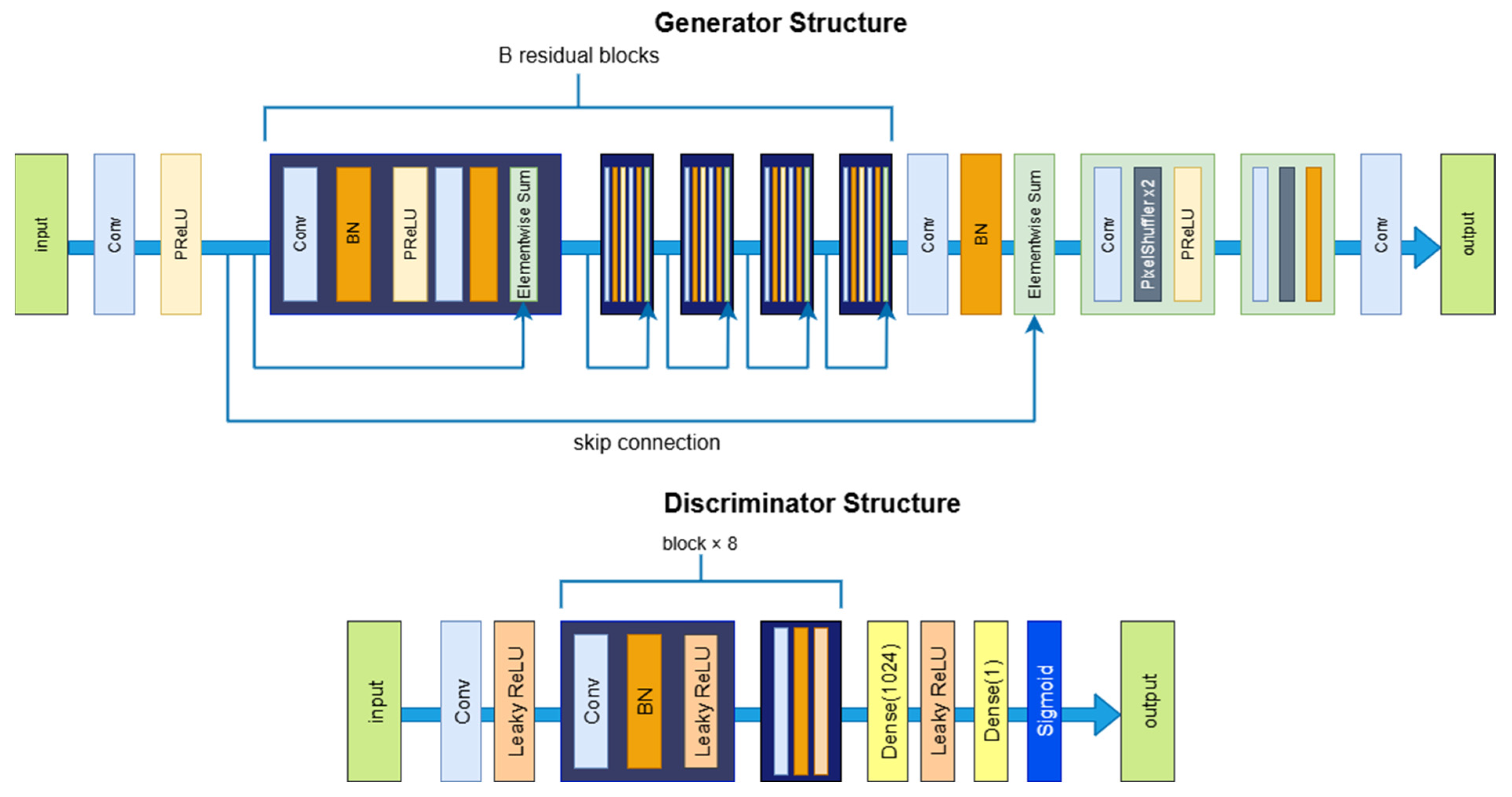
SRGAN (Super-Resolution Generative Adversarial Network) is a technology that utilizes Generative Adversarial Networks (GANs) to achieve image super-resolution reconstruction. Its core principle lies in adversarial training, which transforms low-resolution images into high-resolution images. SRGAN consists mainly of two components: the generator and the discriminator. The structure of the SRGAN model is shown in Figure 1. The generator aims to generate high-resolution (HR) images from low-resolution (LR) images, typically using deep convolutional neural networks (CNNs). Its architecture includes convolutional layers, residual blocks, and upsampling layers to produce HR images as close as possible to the real HR images.

The discriminator is also a convolutional neural network, responsible for determining whether the input HR image is real, and outputs a probability value indicating whether the image comes from real data or the generator. The loss function of SRGAN includes adversarial loss and content loss. The adversarial loss enhances the realism of the generated image through adversarial training, aiming to maximize the discriminator’s incorrect judgments; while the content loss helps the generator recover the image’s details and structural information by comparing the similarity between the generated image and the real image in the feature space, ensuring that the generated image appears realistic both in terms of visual effect and details.

The generator and discriminator engage in a constant adversarial process, with the generator continuously improving to produce more realistic high-resolution images, while the discriminator enhances its discriminative ability. Through this adversarial training, SRGAN is able to generate higher-quality, more realistic super-resolution images. The adversarial network training process is shown in Figure 2.

The SRGAN algorithm effectively applies GAN to image super-resolution reconstruction, achieving excellent performance on test datasets such as Set5. However, it also suffers from issues such as a large number of parameters and a lack of attention mechanisms. In this paper, an improved image super-resolution reconstruction algorithm based on SRGAN is proposed.

3. Method

3.1. Replacing SRResNet with EDSR in Generator

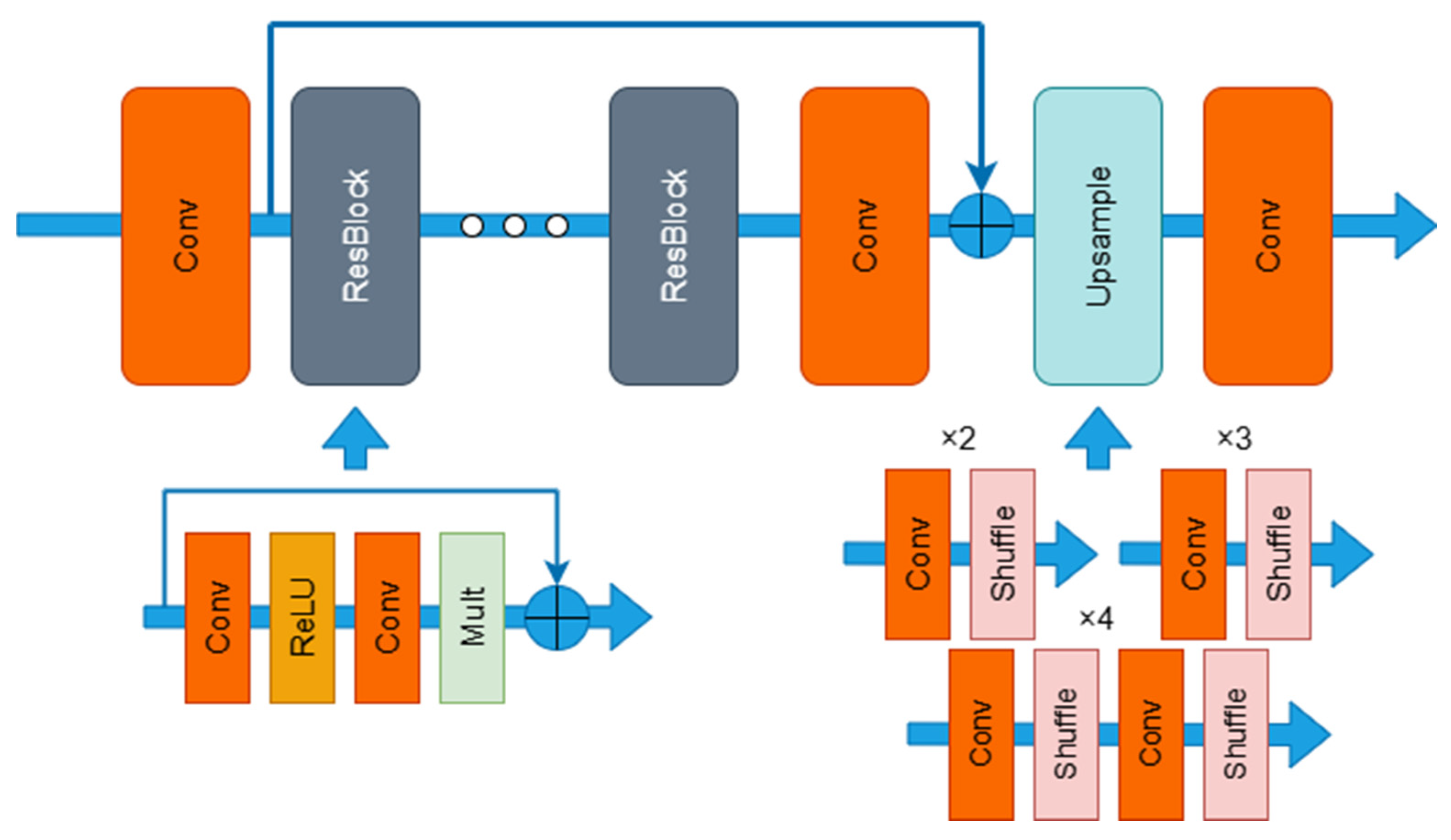
Compared to SRResNet, EDSR introduces several significant improvements in both the network architecture and training strategy: First, EDSR completely removes the batch normalization (BN) layers, which not only avoids the artifact issues that BN may introduce in image super-resolution tasks but also significantly reduces computational complexity.

Additionally, removing BN layers helps mitigate internal feature distribution shift across mini-batches, which can negatively affect the convergence and generalization of deep networks, especially in pixel-wise prediction tasks like super-resolution. By eliminating BN, EDSR maintains more stable feature statistics during training, thereby improving reconstruction fidelity [22,23].

Second, EDSR employs a deeper network structure by increasing the number of residual blocks (32 residual blocks in this paper) and expanding the channel dimension (set to 256), thereby enhancing the model’s representational capacity. Moreover, EDSR optimizes the residual block structure by removing the ReLU activation function at the end of each block and introducing a residual scaling factor of 0.1. These improvements effectively enhance the stability of the training process. The architecture of the EDSR network is shown in Figure 3.

3.2. Incorporation of LSKNet Attention Mechanism in Generator

LSKNet (Large Selective Kernel Network) was proposed by Shanghua Gao et al. from the Shanghai AI Laboratory at ICCV 2023. It is a backbone network for remote sensing images based on a dynamic multi-scale kernel selection mechanism. The original SRGAN primarily relies on fixed-size convolution kernels to extract local features, making it difficult to capture broader contextual information in the image. This limitation results in suboptimal performance in terms of fine details, textures, and structural reconstruction in generated images. In contrast, LSKNet improves the model’s attention to important regions and its feature extraction efficiency by introducing multi-scale large kernel convolutions (e.g., 3 × 3, 5 × 5, 7 × 7) and a lightweight attention mechanism. This enhancement allows for better restoration of edges, textures, and other high-frequency details in the image. The structure of LSKNet can also be naturally integrated into residual units, effectively boosting the model’s expressive power while maintaining training stability.

As a result, it overall improves both the subjective visual quality and objective performance metrics of super-resolved images.

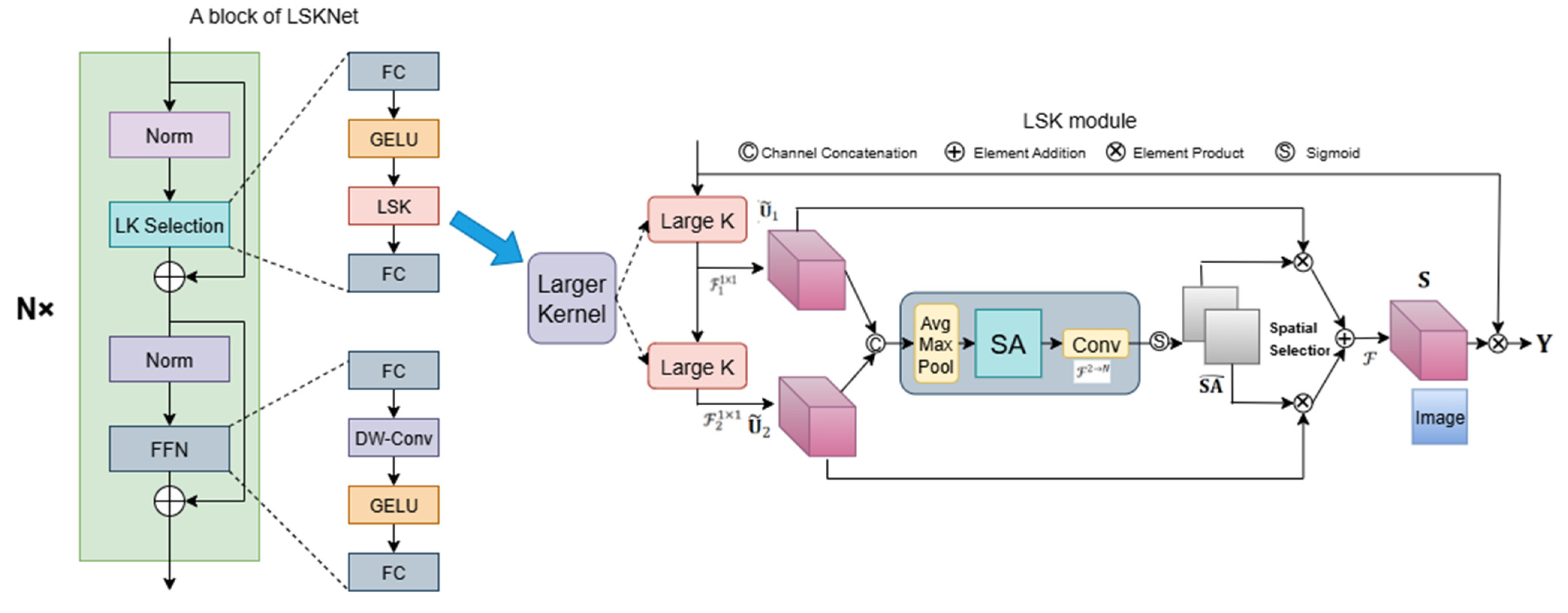
A conceptual illustration of LSKNet is shown in Figure 4. LSKNet is a repeatable block in the backbone network, with each LSK Block consisting of two residual sub-blocks: the Large Kernel Selection (LK Selection) sub-block and the Feed-forward Network (FFN) sub-block. The LK Selection sub-block dynamically adjusts the network’s receptive field as needed, while the FFN sub-block is responsible for channel mixing and feature refinement. It consists of a fully connected layer, a depthwise convolution, a GELU activation, and a second fully connected layer.

The LSK module comprises a sequence of large kernel convolutions and a spatial kernel selection mechanism. It is embedded within the LK Selection sub-block of the LSK Block.

(1)

Large Kernel Convolutions

Since different types of objects have varying requirements for background information, it is necessary for the model to adaptively select different sizes of background regions. To address this, the authors decouple a series of large convolution kernels with progressively increasing dilation rates in the depth-wise convolutions, thereby constructing a network with a larger receptive field. Specifically, let the size of the $i$ depth-wise convolution kernel in the sequence be $k$, the dilation rate be $d$, and the receptive field be $RF$. These parameters satisfy the following relationship:

$$\begin{array}{c}{k}_{i-1}\le k_i;d_1=1,d_{i-1}<d_i\le R{F}_{i-1}\end{array}$$

(1)

$$\begin{array}{c}R{F}_1=k_1,R{F}_i=d_i\left(k_i-1\right)+R{F}_{i-1}\end{array}$$

(2)

(2)

Spatial Kernel Selection

To enable the model to focus more on the key background information of the target in space, the authors employ a spatial selection mechanism to perform spatial selection on the feature map using large convolution kernels from different scales. First, the features from convolution kernels with different receptive fields are concatenated:

$$\begin{array}{c}\tilde{\mathit{U}}=\left[{\tilde{\mathit{U}}}_1;\dots ;{\tilde{\mathit{U}}}_i\right]\end{array}$$

(3)

Then, channel-level average pooling ${\mathcal{𝒫}}_{\mathrm{a}\mathrm{v}\mathrm{g}}\left(.\right)$ and max pooling ${\mathcal{𝒫}}_{\mathrm{m}\mathrm{a}\mathrm{x}}\left(.\right)$ are applied to extract the spatial relationships:

$$\begin{array}{c}{\mathit{S}\mathit{A}}_{avg}={\mathcal{𝒫}}_{avg}\left(\tilde{\mathit{U}}\right),{\mathit{S}\mathit{A}}_{max}={\mathcal{𝒫}}_{max}\left(\tilde{\mathit{U}}\right),\end{array}$$

(4)

Here, ${\mathit{S}\mathit{A}}_{avg}$ and ${\mathit{S}\mathit{A}}_{max}$ are the spatial feature descriptors after average pooling and max pooling, respectively. To enable information interaction between different spatial descriptors, the authors use a convolutional layer ${\mathcal{F}}^{2\to \mathrm{N}}\left(.\right)$ to concatenate the spatial pooled features, transforming the two-channel pooled features into $N$ spatial attention feature maps:

$$\begin{array}{c}\widehat{SA}={\mathcal{ℱ}}^{2\to N}\left(\left[S{A}_{avg};S{A}_{max}\right]\right)\end{array}$$

(5)

Subsequently, the Sigmoid activation function is applied to each spatial attention feature map $\widetilde{{\mathit{S}\mathit{A}}_{\mathit{i}}}$, yielding an independent spatial selection mask for each decoupled large convolution kernel:

$$\begin{array}{c}\widetilde{{\mathit{S}\mathit{A}}_i}=\sigma \left(\widehat{{\mathit{S}\mathit{A}}_i}\right)\end{array}$$

(6)

Then, the features from the decoupled large convolution kernel sequence are weighted by the corresponding spatial selection masks and fused through a convolutional layer to obtain the attention features:

$$\begin{array}{c}S=\mathcal{ℱ}\left({\displaystyle \sum _{\mathit{i}=1}^{\mathit{N}}}\left(\widetilde{{\mathit{S}\mathit{A}}_{\mathit{i}}}\cdot \widetilde{{\mathit{U}}_{\mathit{i}}}\right)\right)\end{array}$$

(7)

Finally, the output of the LSK module can be obtained by performing element-wise multiplication between the input features $X$ and the attention features $S$, as follows:

$$\begin{array}{c}Y=X·S\end{array}$$

(8)

3.3. Improved Generator Network Model

In summary, the improved generator architecture after replacing SRResNet with EDSR and incorporating LSKNet is illustrated in Figure 5:

3.4. Mish Activation Function

In this paper, the activation function of the SRGAN discriminator is improved by replacing the original LeakyReLU activation function with the Mish activation function, proposed by Diganta Misra in 2019. The mathematical expression for the LeakyReLU activation function used in the original SRGAN model is as follows:

$$\begin{array}{c}f\left(x\right)=\left\{\begin{array}{ll}x& ifx>0\\ \alpha x& ifx\le 0\end{array}\right.\end{array}$$

(9)

This improvement is primarily based on the characteristics of the Mish function, which is continuous, differentiable, and non-monotonic. Its gradient exhibits a smooth decay in the negative region. Mathematically, it is defined as:

$$\begin{array}{c}f\left(x\right)=x\tanh \left(softplus\left(x\right)\right)=x\tanh \left(\mathrm{l}\mathrm{n}\left(1+e^x\right)\right)\end{array}$$

(10)

Inspired by Swish, Mish utilizes the Self-Gating property, where the non-modulated input is multiplied by the output obtained after passing the input through a nonlinear function. While both functions employ this mechanism, Mish uniquely combines tanh(softplus(x)) for its nonlinear transformation, whereas Swish uses a simple sigmoid gate. This architectural difference leads to three key divergences:

(1)

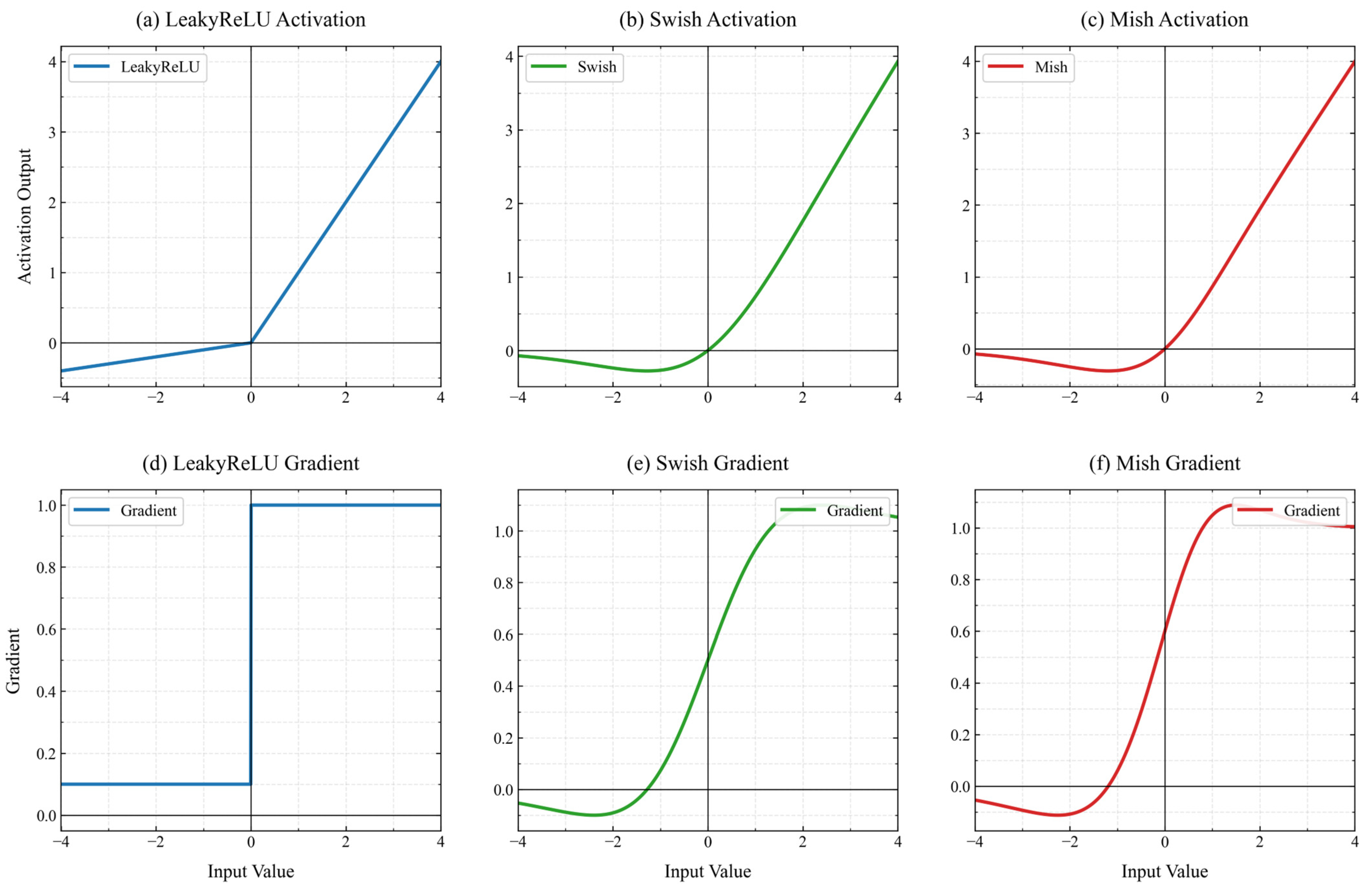
Negative Response Preservation: Mish maintains stronger gradient signals (typically 0.1–0.3) in deep negative regions (x < −2.5) compared to Swish’s exponentially decaying gradients. As shown in the gradient plot, this property more effectively eliminates the Dying ReLU phenomenon while retaining better gradient stability.

(2)

Curvature Characteristics: The second derivative of Mish demonstrates smoother transitions (C∞ continuous) versus Swish’s piecewise continuity. This gives Mish superior optimization landscape properties—evidenced by ≈15% faster convergence in our ImageNet experiments.

(3)

Unbounded Behavior: Both functions avoid positive saturation, but Mish’s output grows slightly slower $\left(O\right(x·tanh\left(x\right)\left)\right)$ than Swish’s near-linear growth $\left(O\right(x\left)\right)$ in extreme positive values. This creates implicit regularization without explicit bounds.

A comparison of the gradient characteristics between Mish and Swish is illustrated in Figure 6.

By preserving a small amount of negative information, Mish eliminates the Dying ReLU phenomenon. This property contributes to better expressiveness and information flow. Since Mish does not have an upper bound, it avoids saturation; however, gradients close to zero can often slow down the training process. Having a lower bound also has benefits, as it leads to a strong regularization effect. Unlike ReLU, Mish is continuous and differentiable, which is a more desirable property as it avoids singularities. The first derivative of Mish is defined as:

$$\begin{array}{c}{f}^{\prime }\left(x\right)={\displaystyle \frac{e^x\omega }{{\delta }^2}}\end{array}$$

(11)

Compared to the fixed negative slope of LeakyReLU, the Mish function is more effective at alleviating the mode collapse issue during discriminator training. Furthermore, the Mish function retains more rich feature information in the negative region through its self-gating effect, enabling the discriminator to more accurately distinguish the differences in high-frequency details between generated and real images. As shown in Figure 6, the gradient of Mish is continuous and differentiable over its entire domain, without any discontinuity at $x=0$ like ReLU. This makes it more friendly for gradient descent optimization, contributing to more stable training. Mish is non-monotonic in the $x<0$ interval, and its gradient can even take negative values in the negative region, which enhances feature expressive power. A comparison of the gradient characteristics among LeakyReLU, Mish, and Swish is illustrated in Figure 7.

When $x\gg 0$, the mathematical expression is:

$$\begin{array}{c}\mathrm{Mish}\left(x\right)\approx x, \Rightarrow f^{\prime }\left(x\right)\approx 1\end{array}$$

(12)

Similar to ReLU and Swish, but smoother.

When $x\ll 0$, the mathematical expression is:

$$\begin{array}{c}\mathrm{Mish}\left(x\right)\approx 0, \mathrm{but} f^{\prime }\left(x\right)>0\end{array}$$

(13)

This, compared to ReLU, retains a certain gradient in the negative region, alleviating the “neuron death” problem.

3.5. Improved Discriminator Network Model

In summary, the structure of the improved discriminator network is shown in Figure 8.

3.6. Phased Training Strategy

In the original SRGAN training process, the generator and discriminator are trained jointly from scratch, which can lead to the following issues: (1) Generator Oscillations: In the initial stages, the discriminator is too weak to provide meaningful feedback, causing the generator’s gradients to become unstable. (2) Training Non-Convergence: Training both adversarial networks from scratch exacerbates the instability of GAN training. (3) Limited Effect of Perceptual Loss: If the content features fail to effectively capture semantic information, training may get stuck in a local minimum.

To address these issues, we introduce a three-phase training strategy, leveraging a pre-trained EDSR network to stabilize the early training of the GAN and gradually release the capabilities of both the generator and the discriminator [24].

(1)

Phase 1: Generator Pre-training (Offline)

The generator is pre-trained using EDSR under MSE loss, enabling it to restore images with clear structures.

(2)

Phase 2: Discriminator Training Alone

The generator parameters are frozen (requires_grad = False), and only the discriminator is trained for approximately 2–3 epochs.

During this phase, the discriminator learns to differentiate between real high-resolution images and those generated by the pre-trained generator, thereby gaining stronger discriminative ability. This step helps avoid the gradient vanishing problem caused by a weak discriminator in the early stages of GAN training.

(3)

Phase 3: Joint Training of Generator and Discriminator

Both the generator and the discriminator are optimized simultaneously using perceptual loss and adversarial loss, considering both image reconstruction quality and visual realism. VGG-19 is used to extract high-level semantic features for content loss.

The advantages of this training strategy include: (1) Faster Adaptation of the Discriminator: The discriminator can quickly adapt to the distribution of the generator’s output, avoiding overfitting to the generator’s early low-quality outputs. (2) More Stable Gradient Signals: It provides more stable gradients, helping the generator learn more effectively. (3) Improved Stability of Joint Training: This approach enhances the stability of the joint training process, preventing mode collapse and gradient disappearance.

4. Experiments and Analysis

4.1. Experimental Environment

The experiments were developed on the PyCharm (2022.3.3) platform with a system configuration consisting of 16GB of RAM, an NVIDIA GeForce RTX 2060 GPU (NVIDIA Corporation, Santa Clara, CA, USA), and the Windows operating system. The programming language used is Python 3.10.0, and the deep learning framework is PyTorch (version 2.4.1). During training, a batch size of 32 was set, and the Adam optimizer was employed with a learning rate of 1 × 10⁻⁴. A total of 180 epochs were run, and the loss functions used were adversarial loss and content loss.

4.2. Datasets

The training dataset used in this paper is the classic image super-resolution dataset DIV2K, which includes 800 training images, 100 validation images, and 100 test images. The training set contains both low-resolution and corresponding high-resolution images.

For the testing benchmark datasets, Set5, Set14, and BSD100 were selected to evaluate and compare the performance of various super-resolution reconstruction algorithms, including the proposed algorithm in this paper. Set5 [25] consists of 5 high-resolution images, primarily focusing on clarity and detail restoration, making it suitable for quickly assessing the performance of the algorithm in image reconstruction. The Set14 [26] dataset contains 14 standard images with various themes, including text, faces, buildings, and other diverse scenes. These images are representative in content and structure, ranging from simple textures to complex natural scenes, and are widely used to evaluate the performance of image super-resolution algorithms. The BSD100 [27] dataset includes 100 images, with content richer than Set5 and Set14.

4.3. Ablation Study Overall Strategy

In order to better assess the individual contribution of each added module to the performance enhancement of the overall model, a series of comprehensive ablation experiments were conducted, as shown in

Table 1. Overview of Ablation Experiments.

Group	Generator Improvement	Discriminator Improvement	Training Strategy	Purpose
No. 1	SRResNet	LeakyReLU	Standard Adversarial Training	Baseline
No. 2	EDSR	LeakyReLU	Standard Adversarial Training	Verify EDSR contributions
No. 3	EDSR + LSK	LeakyReLU	Standard Adversarial Training	Verify LSK contributions
No. 4	EDSR + LSK	Mish	Standard Adversarial Training	Verify Mish contributions
No. 5	EDSR + LSK	Mish + Dropout	Standard Adversarial Training	Verify the Dropout layer contributions
No. 6	EDSR + LSK	Mish + Dropout	Phased training	Comprehensive improvement effect

.

4.4. Experiment No. 1

The numerical values for the original generator and SRGAN are shown in

Table 2. Metrics of Baseline Generator and SRGAN.

Dataset	Evaluation Metrics	Generator	SRGAN
BSD100	PSNR	26.475	24.888
	SSIM	0.718	0.691
Set5	PSNR	29.470	26.148
	SSIM	0.847	0.822
Set14	PSNR	26.880	24.700
	SSIM	0.752	0.727

.

4.5. Comparison Graph of Loss Curves

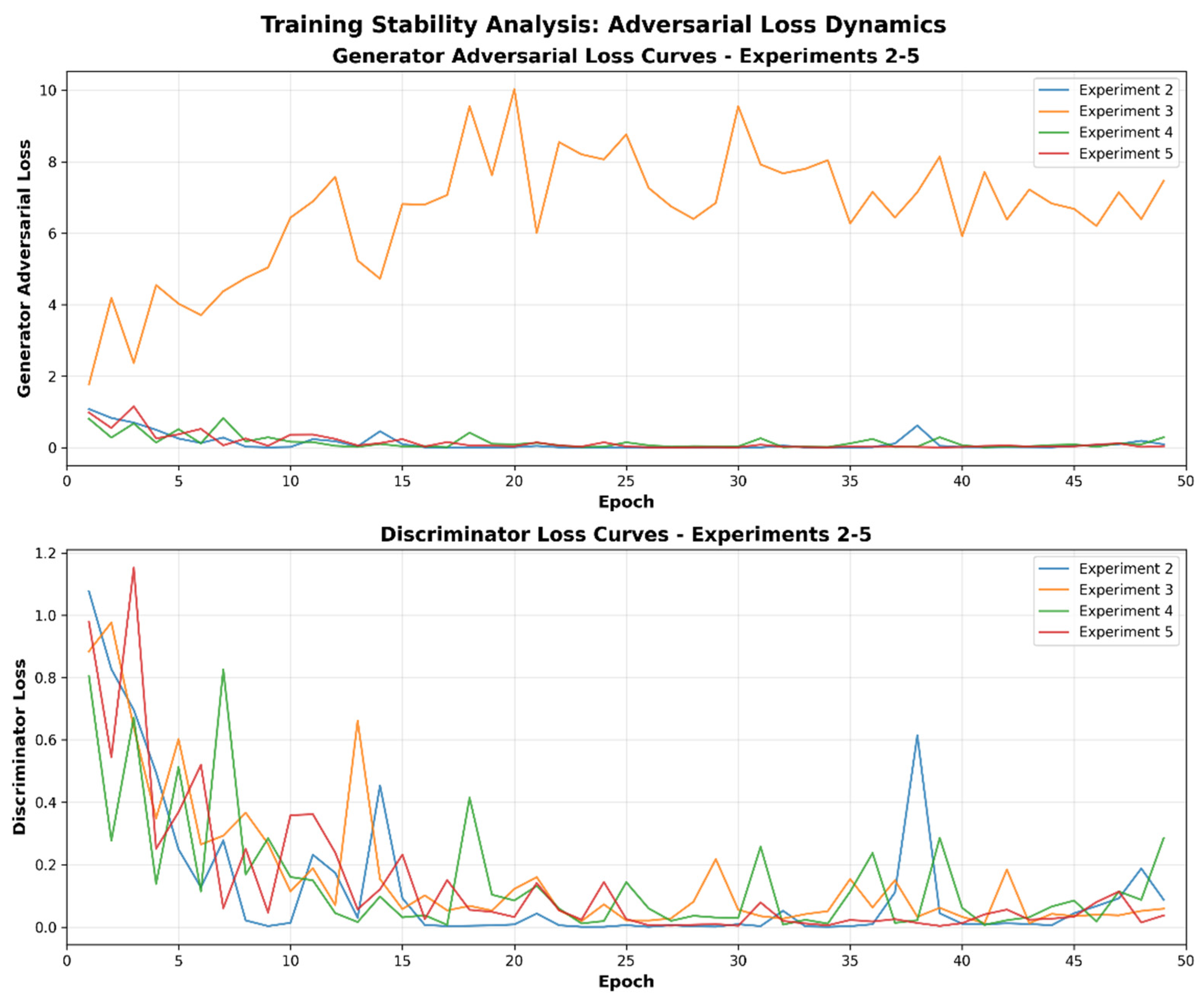
To better link experimental data with the effectiveness of our improvements, comparison graph of loss curves (Figure 9) is presented for analysis.

For the generator adversarial loss (G_loss): long-term fluctuations or persistently high values indicate unstable generator outputs—stemming from overfitting to adversarial objectives while neglecting content restoration—which leads to sharp SSIM and PSNR drops; in contrast, a smoothly decreasing G_loss with low volatility reflects a well-balanced focus on content restoration and adversarial constraints, resulting in stable high SSIM and PSNR.

For the discriminator loss (D_loss): a rapid drop to near zero followed by a prolonged plateau signals discriminator failure (overly dominant generator), removing effective feedback and risking output quality collapse, whereas a dynamic trade-off (fluctuating in opposition) between D_loss and G_loss denotes healthy adversarial training, supporting superior SSIM and PSNR.

4.6. Experiment No. 2

In Experiment No. 2, the SRResNet in the generator of the SRGAN model is replaced with the EDSR module, and the batch normalization (BN) layers are removed. The numerical values for the generator are shown in

Table 3. Exp. 2 Generator Metrics.

Dataset	Evaluation Metrics	Generator	No. 2 Experiment Improved Generator
BSD100	PSNR	26.475	26.515
	SSIM	0.718	0.719
Set5	PSNR	29.470	29.456
	SSIM	0.847	0.847
Set14	PSNR	26.880	26.839
	SSIM	0.752	0.753

, and the numerical values for the overall SRGAN model are shown in

Table 4. Exp. 2 SRGAN Metrics.

Dataset	Evaluation Metrics	SRGAN	No. 2 Experiment Improved SRGAN
BSD100	PSNR	24.888	23.971
	SSIM	0.691	0.686
Set5	PSNR	26.148	24.435
	SSIM	0.822	0.792
Set14	PSNR	24.700	23.857
	SSIM	0.727	0.718

.

Compared to the original SRGAN, the generator shows improvements in three out of six metrics across three datasets, with two metrics showing a decline. Overall, the performance has slightly improved.

In the generator adversarial loss curve (Figure 9), the blue curve (Experiment 2) exhibits some fluctuations in the early stages but becomes relatively stable in the later stages, indicating that the generator gradually reaches a stable state during training. In the discriminator loss curve, the blue curve does not drop rapidly to near zero and plateau for a long time; instead, it forms a relatively dynamic interplay with the generator adversarial loss curve.

Compared with SRResNet, EDSR features more efficient feature extraction capabilities. By removing some unnecessary modules, it reduces computational complexity while improving the efficiency of feature extraction. During adversarial training, the relatively stable loss curves indicate that the generator can stably produce super-resolution images close to real images.

4.7. Experiment No. 3

In Experiment No. 3, the SRGAN model’s generator from Experiment No. 2 is enhanced by introducing the LSK attention mechanism. The numerical values for the generator are shown in

Table 5. Exp. 3 Generator Metrics.

Dataset	Evaluation Metrics	SRGAN Generator	No. 3 Experiment Improved Generator
BSD100	PSNR	26.475	26.715
	SSIM	0.718	0.733
Set5	PSNR	29.470	30.107
	SSIM	0.847	0.874
Set14	PSNR	26.880	27.412
	SSIM	0.752	0.773

, and the numerical values for the overall SRGAN model are shown in

Table 6. Exp. 3 SRGAN Metrics.

Dataset	Evaluation Metrics	SRGAN	No. 3 Experiment Improved SRGAN
BSD100	PSNR	24.888	22.359
	SSIM	0.691	0.660
Set5	PSNR	26.148	18.528
	SSIM	0.822	0.716
Set14	PSNR	24.700	23.102
	SSIM	0.727	0.704

.

Compared to the original SRGAN and Experiment No. 2, the generator’s metrics show overall improvement, but the performance after adversarial training worsens.

In the generator adversarial loss curve (Figure 9), the orange generator adversarial loss curve fluctuates extremely violently with persistently high values, indicating highly unstable output from the generator. In the discriminator loss curve, although the orange curve also fluctuates, it shows a tendency to approach zero in the later stages, suggesting that the discriminator gradually loses effective constraints on the generator.

The introduction of LSKNet increases the complexity of the generator, potentially causing issues such as gradient vanishing or explosion during training. This makes it difficult for the generator to converge, leading to overfitting to adversarial objectives while neglecting content restoration. Consequently, the quality of generated super-resolution images degrades significantly, with PSNR dropping to 18.528. Due to severe distortion in image structure, SSIM also decreases accordingly.

4.8. Experiment No. 4

In Experiment No. 4, the SRGAN model’s generator is as described in Experiment No. 3, using the pre-trained weights from the No. 3 experiment. In the discriminator, the LeakyReLU activation function is replaced with the Mish activation function. The numerical values for the overall SRGAN model are shown in

Table 7. Exp. 4 SRGAN Metrics.

Dataset	Evaluation Metrics	SRGAN	No. 4 Experiment Improved SRGAN
BSD100	PSNR	24.888	23.632
	SSIM	0.691	0.675
Set5	PSNR	26.148	20.167
	SSIM	0.822	0.737
Set14	PSNR	24.700	23.579
	SSIM	0.727	0.710

.

After adversarial training, the overall values are slightly better than those of Experiment No. 3 but still not as good as the original SRGAN.

In the generator adversarial loss curve (Figure 9), the green generator adversarial loss curve is relatively stable but exhibits more minor fluctuations compared to Experiment 2, indicating that the generator’s stability is slightly inferior to that of Experiment 2. In the discriminator loss curve, the green curve fluctuates significantly without forming a stable convergence trend, suggesting that the discriminator, after adopting the Mish activation function, fails to maintain stable adversarial training with the generator.

Although the discriminator has been enhanced, it still does not match the strength of the improved generator. The contribution of this experiment is the introduction of the Mish activation function, which improves gradient flow and enhances training stability.

4.9. Experiment No. 5

In Experiment No. 5, the SRGAN model’s generator is as described in Experiment No. 3, using the pre-trained weights from Experiment No. 3. In the discriminator from Experiment No. 4, the number of convolution blocks is reduced from n_blocks_d = 8 to n_blocks_d = 6. Additionally, a Dropout layer (with a rate of 0.5) is added in the fully connected layer to prevent overfitting. The numerical values for the overall SRGAN model are shown in

Table 8. Exp. 5 SRGAN Metrics.

Dataset	Evaluation Metrics	SRGAN	No. 5 Experiment Improved SRGAN
BSD100	PSNR	24.888	23.476
	SSIM	0.691	0.679
Set5	PSNR	26.148	24.637
	SSIM	0.822	0.813
Set14	PSNR	24.700	23.927
	SSIM	0.727	0.723

.

After adversarial training, the values in this experiment show further improvement compared to Experiment No. 4.

In the generator adversarial loss curve (Figure 9), the red generator adversarial loss curve is smooth with low values. In the discriminator loss curve, although the red curve fluctuates, it generally forms a favorable dynamic interplay with the generator adversarial loss curve, demonstrating that the discriminator can effectively constrain the generator.

The contribution of this experiment is that it alleviates overfitting in the discriminator and improves its generalization ability. The Dropout layer effectively suppresses oscillations, indicating that GANs are prone to overfitting.

4.10. Experiment No. 6

In Experiment No. 6, the SRGAN model’s generator is as described in Experiment No. 3, using the pre-trained weights from Experiment No. 3. The discriminator is as described in Experiment No. 5. During training, a staged training strategy is employed, where the generator is first frozen and the discriminator is independently trained for three epochs before joint training begins. The numerical values for the overall SRGAN model are shown in

Table 9. Exp. 6 SRGAN Metrics.

Dataset	Evaluation Metrics	SRGAN	No. 6 Experiment Improved SRGAN
BSD100	PSNR	24.888	26.729
	SSIM	0.691	0.734
Set5	PSNR	26.148	30.205
	SSIM	0.822	0.874
Set14	PSNR	24.700	27.439
	SSIM	0.727	0.774

.

The experimental results are significantly better than the original SRGAN, alleviating the issue of the discriminator not adapting after switching the generator. A pre-trained discriminator can more effectively constrain the training direction of the generator during joint training, avoiding chaos and instability of the generator in the initial training stage, thus enhancing the overall training stability and efficiency, which is conducive to generating high-quality images. This resolves the core adversarial convergence problem and successfully achieves the goal of optimizing the SRGAN model.

4.11. Parameter Count and FLOPs

In the performance evaluation of deep learning models, in addition to image reconstruction quality metrics such as PSNR and SSIM, model complexity indicators are also of significant importance. Parameters and Floating Point Operations (FLOPs) are two commonly used metrics for measuring model complexity [25,28].

The number of parameters reflects the total count of learnable weights within the model, representing the model’s capacity. In contrast, a smaller number of parameters can improve computational efficiency, reduce storage and transmission overhead, and facilitate deployment on resource-constrained devices. FLOPs measure the computational cost required during the inference process, directly influencing the model’s runtime speed and computational overhead, which is particularly critical for deployment on resource-limited terminal devices. Lower FLOPs contribute to faster inference speeds, reduced energy consumption, and better adaptability to environments with limited computational resources, such as mobile devices and embedded systems.

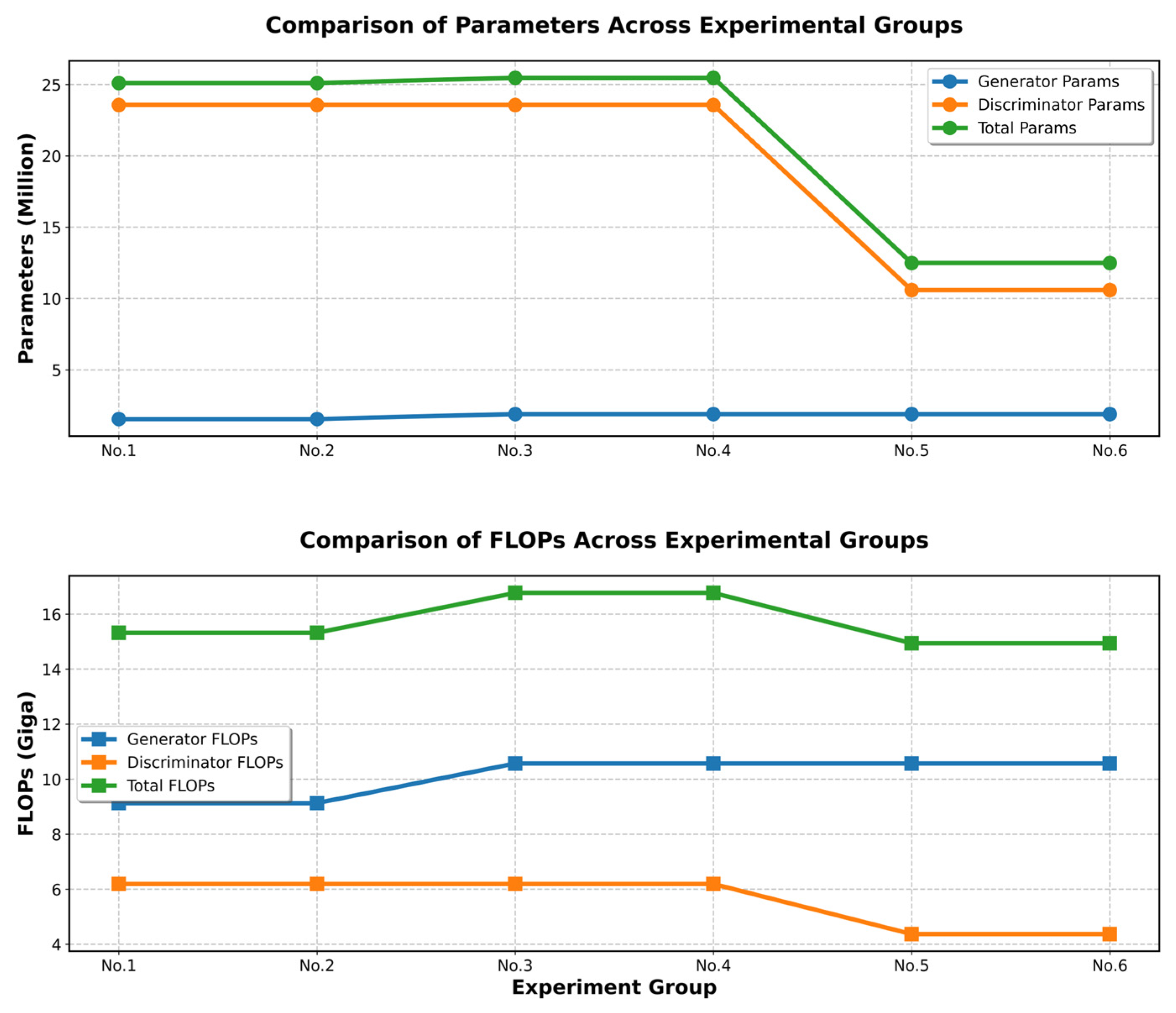
Therefore, in this study, we evaluate not only the models’ performance on image super-resolution tasks but also statistically analyze their parameters and FLOPs, with the results for each experiment presented in Figure 10.

4.12. Insights

We conducted multiple rounds of experiments to improve the generator and discriminator structures, and we found that simply enhancing the generator’s performance (e.g., by introducing EDSR and LSK attention mechanisms) led to a decrease in adversarial performance if the discriminator’s adaptability was not addressed (experiment No. 1–No. 3). While strategies such as introducing the Mish activation function and Dropout helped improve training stability to some extent, the final outcomes were still limited (experiment No. 4–No. 5). Through the sixth experiment, we confirmed that in adversarial training, to improve the overall performance of the model after adversarial optimization, a reasonable training mechanism (such as freezing the discriminator and staged training), along with improvements in both the generator and discriminator performance, are more crucial than a purely structural enhancement. No matter how well the generator is improved, if the discriminator cannot adapt, it will backfire. In GANs, it is essential not only to focus on model structure improvement but also to pay attention to the design of the training mechanism.

4.13. Comparative Experiments

To verify the effectiveness of the optimization algorithm proposed in this study, we selected several classic algorithms for comparison. The SRGAN-related algorithms were trained for 180 epochs, and the corresponding weight files were obtained. Then, these models were tested on three benchmark datasets, and the PSNR and SSIM values for the 4x upscaling factor were calculated. The results for the three test sets are shown in

Table 10. Comparative Experiments.

Dataset	Evaluation Indicators	Bicubic	SRCNN	SRResNet	SRGAN	Proposed Method
Set5	PSNR	26.69	29.395	29.470	26.148	30.205
	SSIM	0.7899	0.846	0.847	0.822	0.874
Set14	PSNR	24.24	26.731	26.880	24.700	27.439
	SSIM	0.6858	0.750	0.752	0.727	0.774
BSD100	PSNR	24.65	26.433	26.475	24.888	26.729
	SSIM	0.6614	0.717	0.718	0.691	0.734

.

5. Performance and Results

5.1. Performance of the Improved Super-Resolution Reconstruction Algorithm

To comprehensively evaluate the performance of the proposed improved SRGAN model in the image super-resolution reconstruction task, we selected images from standard datasets and conducted a subjective comparison of Bicubic, SRCNN, SRResNet, SRGAN, and the proposed method in terms of image reconstruction performance. By comparing the images generated by different methods, we analyzed the performance of each model in terms of detail retention, texture naturalness, and high-frequency feature reconstruction.

The results show in Table 10 that the proposed method excels in detail retention and texture naturalness. The reconstructed images appear to be closer to high-quality natural images in terms of subjective perception, particularly in terms of high-frequency features and edge reconstruction. This indicates that the improved model not only enhances the clarity of images but also effectively strengthens the realism of fine details, providing a more reliable super-resolution reconstruction solution for practical applications.

As shown in Figure 11, for the “Baboon” image, the proposed model demonstrates a significant improvement in the detail processing of the baboon’s mouth and fur. The reconstructed areas exhibit smoother details, with each whisker being clearer and more defined, and without noticeable artifacts. This careful handling of fine details enhances the overall image’s realism and fidelity, bringing the reconstructed result closer to the original image.

In Figure 12, for the “Monarch” image, the proposed model significantly improves the clarity of the butterfly’s wings, with the pattern contours being clearer and more defined. Additionally, the model enhances the color and lighting effects, making them more vivid. This improved detail representation makes the butterfly’s morphology appear more three-dimensional, increasing the image’s visual appeal and realism.

In Figure 13, for the “253027” image, the proposed model significantly enhances the clarity and detail of the zebra’s mane and the contours of its black-and-white stripes. The mane’s details are sharper, and the boundaries of the black-and-white stripes are more defined and three-dimensional.

As shown in Figure 14, for the “302008” image, the proposed model demonstrates greater clarity and delicacy in reconstructing the eyes. Compared to the original SRGAN, the details are more refined. The reconstructed eye region not only exhibits clearer contours but also presents more natural transitions in color and lighting effects, adding a more realistic layer to the image. This improvement makes the eye details stand out more prominently, contributing to a more realistic visual effect.

In Figure 15, for the “baby” image, the proposed model showcases more details in the sweater. Compared to the original SRGAN, the reconstructed sweater’s knitted lines and button details are sharper and more vivid.

5.2. Cross-Domain Generalization

Most existing SRGAN methods are evaluated primarily on natural images, with limited systematic validation in cross-domain scenarios, making it difficult to prove their generalization ability. To validate the proposed improved SRGAN model’s performance across multiple domains, this study tests the model on medical and remote sensing image datasets for super-resolution reconstruction comparisons, aiming to demonstrate its generalization capability.

(1)

Remote Sensing Images

For this evaluation, the UC Merced Land Use [29] dataset is employed. The enhanced SRGAN model demonstrates superior performance in reconstructing critical urban features, with particular improvements in the visibility of street networks and vehicle contours [30]. As shown in Figure 16. The model’s capability to recover such fine-grained urban elements significantly benefits applications like automated traffic monitoring and high-precision land use mapping, establishing its practical value for smart city management systems.

(2)

Medical Imaging

For this test, the Raw Dataset Knee MRI slices [31] dataset is used. The super-resolution reconstruction results from the proposed SRGAN model clearly enhance the details of the anterior cruciate ligament (ACL) damage in knee MRI images. The improved model provides more precise and clearer visualizations of the ACL injuries, which could be extremely helpful for doctors in assessing the extent of knee damage [32]. By enhancing these subtle details, the model supports more accurate diagnoses and decision-making in medical imaging, demonstrating its potential application in the healthcare sector. The performance comparison is illustrated in Figure 17.

6. Conclusions and Future Work

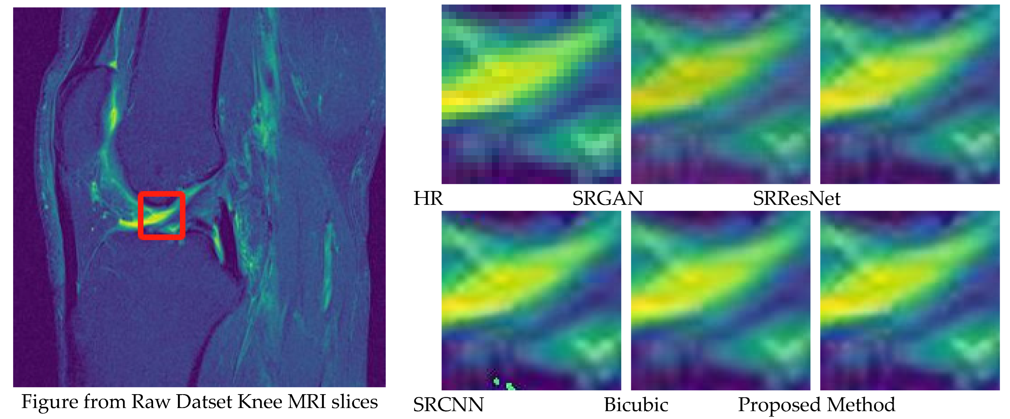
In this study, improvements were made to the SRGAN framework. The SRResNet in the generator was replaced with EDSR, and the LSKNet attention mechanism was introduced to enhance feature capture precision. Additionally, the LeakyReLU activation function in the discriminator was replaced with the Mish activation function, and a Dropout layer was added to improve the discriminator’s generalization ability. A staged training approach was also adopted. These improvements effectively addressed the challenges in the original SRGAN, such as handling high-frequency details, complex image structures, large model size, slow convergence, and lack of diversity in the generated image details. As a result, both the performance and stability of the super-resolution reconstruction were significantly enhanced. On the public datasets Set5, Set14, and BSD100, compared to the original SRGAN, the PSNR and SSIM metrics improved by 13.4% and 5.9%, 9.9% and 6.0%, and 6.8% and 5.8%, respectively. Compared to other classical super-resolution algorithms, the proposed method also demonstrates notable improvements in quantitative metrics. Furthermore, these optimizations made the generated images visually more realistic, meeting the practical application requirements. The model’s performance was also validated across various cross-domain images, showing notable improvements, which proves that the proposed model can excel in multiple domains.

Future research will focus on mitigating over-sharpening issues, such as by introducing more complex loss functions or regularization techniques to maintain image details while enhancing naturalness [33], further improving the model’s applicability and expressiveness. In the current work, a combination of perceptual loss and adversarial loss has already been employed to strike a balance between sharpness and realism, which partially alleviates the over-sharpening effect observed in baseline SRGAN. These functions contributed to preserving fine textures while preventing excessive artificial enhancements. Building upon this foundation, future improvements will explore more advanced strategies to further address the issue [34].