Abstract
This paper addresses the challenges of testing computing systems and their hardware components, especially memory devices. It highlights the limitations of traditional random testing. Such methods often fail to use available information about the system under test and previously generated test patterns. The potential of controlled random testing, which incorporates knowledge of prior patterns, is therefore explored. A class of controlled random tests with a limited number of test patterns is identified and analyzed, including existing standard approaches. The paper introduces a novel measure of dissimilarity between test patterns. This measure is based on calculating Hamming distances for binary patterns after mapping them into different numeral systems, including quaternary, octal, and hexadecimal. We propose a method for generating controlled random tests with a guaranteed minimum Hamming distance. It is based on representing binary patterns as symbols from non-binary numeral systems. In this way, ensuring a specific Hamming distance in the symbolic domain also guarantees at least the same distance in the binary representation. We evaluate the effectiveness of the proposed method through simulations, particularly in the context of memory testing and the detection of multicell faults, i.e., errors caused by interactions between multiple memory cells. This approach can enhance the efficiency and reliability of test procedures in embedded systems, memory diagnostics, and safety-critical applications.
1. Introduction
Testing is still the main method used to verify the quality of software, hardware, memory devices, and applications. Even though many design-for-test and analysis methods have been proposed, testing remains a process that requires considerable effort and time. Therefore, systematic and automated procedures for generating test data are very important. Since the 1960s, probabilistic approaches, usually called random testing, have been widely used because they are simple to understand and easy to apply [1,2,3]. However, the efficiency of purely random methods is low: they usually ignore information about the system under test and about earlier test patterns, which often results in weaker fault detection [4,5].
To overcome this limitation, different controlled versions of random testing have been developed. In this paper, we use the term controlled random testing (CRT) [6] for methods that select the next pattern based on its difference from the previous ones. The Hamming distance is most often used as a measure of this difference. A related idea, well known in software testing, is called adaptive random testing (ART). A more detailed overview of these approaches is given in Section 2.1, while the theoretical background relevant for CRT is presented in Section 2.2.
The main problem studied in this paper is the choice of a difference measure that (i) can properly describe the diversity between test patterns and (ii) can be computed with low complexity [5,7]. The classical Hamming distance is widely used, but it often treats different patterns as equally distant, even when their structures are sufficiently different. To address this, we propose to extend the idea of Hamming distance by interpreting binary patterns in other numeral systems and by defining a new vector-based dissimilarity measure. This allows us to construct controlled tests that remain efficient to compute but can better distinguish between candidate patterns.
Contributions. The paper offers the following contributions. First, we introduce a framework in which an n-bit binary pattern can be mapped to sequences over alphabets of higher radix while still allowing for distance calculations in a consistent way. Second, we define a new vector-based dissimilarity measure based on these representations and discuss its main properties. Third, we propose a method for generating controlled random tests with a given minimum Hamming distance that reduces the need for expensive candidate checks. Finally, we show in experiments with memory-oriented examples that our method provides a more effective selection of patterns at a reasonable computational cost.
Paper organization. Section 2 is divided into two parts. Section 2.1 reviews earlier work on controlled random testing. Section 2.2 presents the coding-theoretic background and shows bounds that limit the construction of CRT. Section 3 introduces the representation-based extensions of the Hamming distance and the new dissimilarity measure. Section 4 describes the method for generating tests with a given minimum Hamming distance. Section 5 presents the experimental results, and Section 6 gives the conclusions and future directions.
2. Controlled Random Tests Analysis
2.1. Related Work
The related work can be grouped into three major streams: (i) pseudo-random and pseudo-exhaustive testing, (ii) diversity-driven methods such as Antirandom Testing and its extensions, and (iii) adaptive random testing (ART) and its numerous variants. Below, we summarize key contributions within each stream.
Random testing has long been applied in hardware and memory verification due to its simplicity and low implementation cost. In practice, purely random vectors are seldom used directly; instead, pseudo-random sequences are commonly employed, often generated by linear feedback shift registers (LFSRs) within built-in self-test (BIST) schemes [8]. Exhaustive and pseudo-exhaustive approaches have also been investigated to guarantee high fault coverage [9]. Early seminal work by McCluskey [10] introduced a pseudo-exhaustive testing methodology that became a foundation for later approaches. Fujiwara [11] provided further theoretical and practical developments, placing pseudo-exhaustive methods within a broader framework of logic testing and design for testability. Karpovsky, Yarmolik, and van de Goor [12] subsequently applied pseudo-exhaustive techniques to RAM testing, demonstrating their potential for memory devices. While such methods ensure thorough fault coverage, they are impractical for large memories due to excessive computational requirements. Such drawbacks motivated the development of more advanced approaches that explicitly control the diversity of generated test patterns.
A significant breakthrough was the introduction of Antirandom Testing by Malaiya [13,14,15], who first defined and demonstrated the method as a distance-based black-box testing strategy. Yin [16] subsequently developed a practical tool for generating hardware test sequences based on the principle of maximizing dissimilarity between test vectors, providing one of the earliest implementations of the antirandom concept. The idea of maximizing dissimilarity was later refined through extensions, including, among others, Fast Antirandom Testing (FAR) [17], Scalable Antirandom Testing (SAT) [18], and Pseudo-Ring Testing (PRT) [19]. Notably, most of these extensions were developed in the context of hardware and memory testing.
In parallel, the concept of selecting tests according to their distance from previous ones was generalized into what became known as adaptive random testing (ART) [20,21,22]. Unlike the earlier hardware-oriented approaches, ART and its numerous variants were primarily investigated in software testing. These include Good Random Testing [23], Restricted Random Testing [24,25], Maximum Distance Testing [26], Mirror Random Testing [27], Orderly Random Testing [28], hybrid adaptive random testing [29], and Evolutionary Random Testing [30], among others. A variety of distance metrics have been explored in this context, including minimum, average, maximum, centroid-based distances, discrepancy, and membership grade, as well as Hamming distance [7]. None of these metrics can be regarded as predominant across all ART variants, but they share the common goal of enforcing diversity when selecting new test cases. Comprehensive surveys, such as Anand et al. [5] on automated test case generation, Grindal et al. [31] on combination and diversity-driven strategies, Chen et al. [32] and Huang et al. [7] on adaptive random testing, and Feldt [33] on quantifying test diversity, provide broader overviews of these approaches and underline the central role of diversity metrics in general.
Despite these contributions, most existing methods still rely on evaluating specific characteristics of previously generated test sets. The vast majority of the approaches presented share the common goal of maximizing diversity among test patterns. However, this goal is most often achieved at the expense of increased computational overhead [34]. While such costs may be acceptable in some software testing contexts, they become a serious limitation in hardware- and memory-oriented testing, where the efficiency of test generation is a critical requirement. Therefore, there is a clear need for methods that ensure sufficient diversity of test patterns while significantly reducing the computational burden.
2.2. Formal Analysis of Controlled Random Tests
Following the discussion of related work, this subsection provides a theoretical background on controlled random tests (CRTs). The analysis emphasizes the role of Hamming distance as the principal diversity metric and introduces fundamental bounds and constructions that shape the efficiency of CRT generation. The presented considerations are rooted in the classical results of coding theory, including Hamming’s seminal work on error-detecting and error-correcting codes [35], the comprehensive treatment by Peterson and Weldon [36], and the Plotkin bound [37], while also extending our earlier research on Multi-Run Memory Tests [38] and optimal controlled random tests [39].
In the following discussions, we consider a sequence of data as a test pattern consisting of n elements , where generally represented in an arbitrary alphabet. As shown in [7], the next test pattern in a controlled random test is designed to differ as much as possible from the previously generated patterns . The hypothesis assumes that for two test patterns with the maximum difference, the number of faults (errors) detected by the second pattern will also be maximized. The Hamming distance for is often used as a criterion to distinguish the test pattern from the previous patterns [7,32].
For the general case, the Hamming distance is calculated by comparing two sequences of data, and each consisting of n characters and from an arbitrary alphabet [35,36].
The Hamming distance between and is defined as the number of positions at which and differ, and it can be expressed as
where
When comparing n characters in the patterns and , the minimum value of the Hamming distance, , is 0 if all characters match, and the maximum value, , is n if all n characters differ. For example, in the case of binary number systems, the Hamming distance between and is 2, as they differ at two positions.
Most commonly, binary test patterns are considered, but they can also be interpreted as sets of characters from other alphabets corresponding to different numeral systems. For example, quaternary, octal, hexadecimal, and other alphabets can be used, where a fixed number of consecutive bits in the original binary patterns represent the binary code of a character in the corresponding alphabet. For instance, the binary pattern , when divided into groups of two consecutive bits, can be represented in the quaternary number system, which uses an alphabet of four characters (0, 1, 2, and 3), as . In the hexadecimal system, the same pattern takes the form .
The main idea behind most approaches to controlled random test generation is to select, from a given set of test candidates, the pattern that has the maximum Hamming distance with respect to the previously included patterns . Various criteria can be used for selecting ; however, the most common is to maximize the value of , where . In this case, the generated test will be characterized by the minimum Hamming distance between any two test patterns included in the test [7]. As a result, the controlled random test is defined by the value of the minimum Hamming distance, as described in the following definition.
Definition 1.
The value for a controlled random test is equal to the minimum Hamming distance between two arbitrary test patterns and , where and .
In terms of coding theory, the characteristic can be regarded as the code distance d of the code , which represents the smallest Hamming distance between different pairs of code words . Therefore, based on the fundamental principles of coding theory, several useful conclusions can be drawn that must be considered when generating controlled random tests.
In particular, a significant feature of controlled random tests is their limited length. This follows from the fact that the larger the minimum distance , used as a criterion for including in the test, the fewer patterns exist that satisfy this criterion. This relationship is described by the Hamming bound [35,36].
Hamming Bound. The estimation of the Hamming bound for , where r is an integer, can be expressed as the inequality:
Here, the Hamming bound denotes the maximum possible size q of a b-ary block code T of length n and minimum Hamming distance d between code words. In the context of controlled random tests, the value directly affects the test length. For example, in the case of binary patterns () with and , the Hamming bound can be calculated as
As shown in this example, increasing the Hamming distance to a value of 7 reduces the estimate of q to 2. This means that the controlled random test T for and will consist of no more than two patterns: and . It is important to note that the pattern is generated randomly and can take any of binary values, while the second pattern is selected to satisfy the criterion . Thus, there is a large variety of controlled random tests T with , but each test consists of only two patterns: and . In practice, this result shows that for short memory words, only a very limited number of maximally distant test patterns can be constructed, which restricts the applicability of such strict distance requirements.
Let us consider approaches for constructing controlled random tests consisting of a minimal number q of test patterns, for which takes the maximum possible value.
For the synthesis of controlled random tests with a small number of patterns q, we first examine classic codes with [37]. It is known that the Plotkin theorem allows for determining the maximum possible number q of code words in a binary code of length n with . The Plotkin bound provides an upper limit for this value [37,39].
Plotkin Bound. If and n is even, the following inequality holds for q:
For odd values of n, the Plotkin bound is expressed as
Based on the application of the Plotkin bound, a formal algorithm for synthesizing controlled random tests , characterized by a small number q of patterns with the maximum–minimum Hamming distance between test patterns and , is proposed in [38].
For , based on (3) and (4), the maximum possible value of the distance can be estimated. This result, , and the corresponding test is supported by previous findings for the optimal random test consisting of two inverse patterns, and [35,36].
In the case of , according to the Plotkin bound, . As shown in [38], the closest optimal solution can be achieved only for , where . For , the test can be constructed with [38].
By generalizing the heuristic procedure for constructing for small values of q, a formal algorithm for synthesizing the test for a given was presented in [38]. According to this algorithm, the test consists of q patterns with
It should be noted that for any integer q, the distance is greater than ; however, as q increases, it approaches .
A very important remark concerns the size n of the test patterns, which must be considered. In order to generate tests with , the value of n must be divisible by , and its minimal value is . For example, in the case of , one variant of the test is with the minimal value .
Based on the Hamming distance for test patterns and , and their Cartesian distance as described in [39], a method for synthesizing optimal controlled random tests (OCRTs) is considered. These tests are characterized by the conditions and . In the general case, the number of OCRT patterns is defined as A constructive algorithm for generating test patterns is presented in [39]. For the specific case when , where m is an integer, the number q of OCRT patterns is given by . For example, when , the number of OCRT patterns is , and for , the number of patterns is .
The example of the test with for presented in [38] and the OCRT for are shown in Table 1.

Table 1.
Examples of MMHD(4) for and OCRT with tests.
These small examples demonstrate how theoretical bounds directly limit the number of feasible patterns in controlled random tests, especially for memory diagnostics where compact but diverse test sets are needed. At the same time, the and OCRTs shown in Table 1 can be interpreted as templates for generating patterns of similar tests. A specific or OCRT can be defined by a randomly chosen initial test pattern , based on which subsequent patterns are generated by inverting the bits of according to the given templates. For example, in the case of shown in Table 1, if the random initial pattern is chosen as , the corresponding new test will consist of the patterns . Therefore, in the following text, the abbreviation is used to denote a family of tests with q test patterns and the corresponding value of .
A common drawback of both approaches to generating controlled random tests, MMHD and OCRT, is the limitation and restriction on the size of their test patterns. Four main algorithms are known for constructing a set of test patterns (code words) with given properties based on an initial test (code) [36]. These algorithms utilize the following four properties, which we formulate for the case of [36].
Property 1.
The result of permuting the bits simultaneously in all q test patterns of the test is the test .
Property 2.
The result of inverting the bits in all q test patterns of the test is also the test .
Property 3.
The test with test patterns
consisting of bits, is obtained from the test pattern of the original test by concatenating it (repeating) u times. For example, if , then
Property 4.
The result of scaling (increasing) by s times the test is the test , consisting of test patterns , where is the test pattern of the original test .
The results of applying the above properties to the test shown in Table 1 are illustrated in Table 2.
Table 2.
MMHD(4) test extension examples.
The presented analysis of controlled random tests with a small number of test patterns demonstrates the feasibility of generating such tests without significant computational costs. The examples provided in Table 2 illustrate the derivation of new controlled random tests using formal methods, which enable the generation of a new set of test patterns as well as the adjustment of the pattern size n. It should be noted that the given properties apply not only to the and OCRT but also to any controlled random tests.
As noted above, the key characteristic of tests with a small number of test patterns is the relationship between the value of the Hamming distance and the number q of test patterns. Increasing the required minimum Hamming distance —essentially maximizing it—reduces the number q of patterns in the generated test. It is evident that both test parameters, namely, the Hamming distance and the number of test patterns, influence the efficiency and quality of the test. Intuitively, one might conclude that increasing both parameters improves the test properties. Indeed, the more test patterns that are maximally distant from each other, the more efficient the test becomes. However, as the analysis above has shown, it is impossible to simultaneously increase both parameters. Therefore, in the subsequent discussion, we will consider an approach that focuses on increasing the number of test patterns while maintaining the minimum Hamming distance at an acceptable level.
In summary, the theoretical analysis highlights a fundamental trade-off: increasing the minimum Hamming distance between test patterns inevitably reduces the number of patterns in the test. These coding-theoretic constraints motivate the search for alternative distance measures, which can better balance diversity and efficiency. Section 3 introduces representation-dependent interpretations of the Hamming distance, aimed at achieving this balance.
3. Modified Approach to Hamming Distance Calculation
The Hamming distance has significant limitations as a dissimilarity metric, as it only distinguishes fully matching patterns and with while treating all other non-identical patterns equally. One argument that confirms the indistinguishability of non-matching sequences is the case of binary patterns and , for which the Hamming distance is always constant and equal to n. For example, As seen above, the Hamming distance in all the given examples is equal to , indicating the same maximum difference across all pairs of patterns. However, the structural differences between these pairs of sequences are significant. An even greater structural difference exists in the following character sequence pairs, for which the Hamming distance is . These examples highlight the need for alternative dissimilarity measures capable of capturing not only the number of differing bits but also the spatial and structural relationships within the sequences.
Let us examine the potential for extending the use of Hamming distance in comparing finite sequences of characters and , which represent test patterns consisting of n characters (elements) and , where . The alphabet of characters and can be arbitrary, as well as the number n of elements in the patterns and . Without loss of generality, we assume that the test pattern is initially a binary pattern, meaning that the characters .
The primary objective of the existing modifications to the Hamming distance calculation is to select, from among potential test pattern candidates, a test pattern that is most different from the previously included pattern .
The first modification assumes that the length of a binary test pattern is restricted to , where w is an integer. Such constraints frequently occur in practice when addressing diagnostic problems in computer systems. Under this condition, the original binary sequence
can be represented in different ways denoted as , where . The index specifies the number of consecutive bits that form each character in the new alphabet. For (), we obtain the binary alphabet:
For (), we obtain the quaternary alphabet:
where each character is formed from two consecutive bits of . For larger values of v, the construction continues in the same manner, producing
In the general case, the sequence consists of characters. Each character of this alphabet is obtained by concatenating two neighboring characters of the previous representation . For instance, for :
and, more generally,
Thus, each representation defines a sequence over a different alphabet, offering multiple perspectives on the same original binary pattern.
The given interpretation of the original binary patterns does not prevent the determination of the Hamming distance between the patterns and . Just as in the case of binary vectors, Equation (1) can also be applied here, provided that both patterns are expressed in the same chosen alphabet. Let us illustrate this with the following example for the case where .
Example 1.
As an example of binary test patterns, consider and , for which the condition is satisfied. For each pattern of binary characters and , in accordance with the above-described definitions, there are representations in the form of sequences of characters belonging to different alphabets (see Table 3).
Table 3.
Hamming distance computation in multiple alphabets for n = 8.
In Table 3, the Hamming distance for the original binary patterns and , as well as for their representations in different alphabets with their respective characters, is presented. In this example, ASCII codes are used to represent and . For all cases, the value of the Hamming distance has been calculated based on Equation (1). The resulting characteristic , represented by the four components , provides a more accurate assessment of the differences between these test patterns.
The requirement that the dimension of a binary pattern , where w is an integer, may not always be satisfied in practice. Consequently, for cases where , when mapping the original pattern into the sequences , the required number of bits equal to may be insufficient for the last character of the sequence , where . For example, considering the pattern , where , it can be represented as the sequences and . However, in three cases—, , and —the required number of bits is insufficient for the last character of the corresponding alphabet; specifically, one bit is missing for , and one bit is missing in both and . An obvious solution to overcome this limitation is a cyclic interpretation of the original pattern . This interpretation assumes that the bit following the last bit is the first bit , thereby using the initial bits of the pattern to obtain the required number of bits for the last character of . For the pattern , such an interpretation allows us to obtain .
The notation above, as well as the symbols “c” and “[” in Table 3, represent values in the base-256 numeral system. In each case, a group of 8 consecutive bits is interpreted as a single element of a 256-ary alphabet. Thus, is represented by (ASCII code for the letter b), while and correspond to the ASCII symbols “c” and “[”, respectively. It should be emphasized that these ASCII representations are used only as illustrative examples, since the base-256 system also includes non-printable and control characters. The purpose of this notation is to demonstrate that every 8-bit block can be treated as one symbol of a base-256 alphabet.
Removing the restriction on the size n of the binary pattern by extending it to the required number of bits allows for an expansion in the number of alphabets available for different mappings of the original pattern. Naturally, considering the possibility of extending the original binary pattern to the required number of bits, the number of alphabets can be increased up to n. These alphabets consist of characters specified by one bit, two bits, three bits, four bits, and so on, up to the alphabet in which each character is determined by n consecutive bits. For example, considering the original pattern with and its cyclic extensions, it can be represented in the form of sequences obtained for different alphabets. The sequential representations are as follows: , , , , and .
Another approach to representing the original test pattern in various numerical systems with different character sets is to expand the last character of the pattern by appending, for example, all zero values. Consider the example of a test pattern , which can be represented in five different numerical systems, each with its own alphabet. To avoid potential conflicts related to the absence of a complete set of characters (or their graphical representation) in alphabets containing a large number of symbols, each character in all numerical systems will be represented in binary form and separated by spaces. Thus, the test pattern can be represented in five different numerical systems as follows: .
Let us define the binary n-bit test pattern as a pattern in a numerical system other than binary.
Definition 2.
The test pattern , consisting of n binary characters, can be interpreted in a numerical system with characters as the pattern , where . This pattern consists of characters, where is expanded to a size of bits by adding zeros.
For example, the test pattern with can be represented in the octal () numerical system with characters as . To achieve this representation, zeros have been added.
Note that the above examples of interpreting the pattern and Definition 2 allow us to consider binary test patterns in various number systems. Using the last example of representing the test pattern in different number systems, let us illustrate the determination of the Hamming distance (Equation (1)) for each interpretation of two patterns: and .
The below example (see Table 4) of determining the Hamming distance demonstrates the possibility of obtaining, based on Equation (1), several numerical assessments of the relationship between the original binary patterns and .
Table 4.
Example of the Hamming distance calculation.
Let us now define a new measure of dissimilarity between the binary test patterns and , which consists of a set of numerical characteristics represented by the Hamming distances.
Definition 3
(Dissimilarity Measure ). The dissimilarity measure between two binary test patterns and , where and , is defined as an n-component vector composed of the Hamming distances
calculated according to Equation (1).
The analyzed characters and of the test patterns and , according to Definition 2, are represented by binary bits. Accordingly, using Equation (1), the numerical values of the components of the dissimilarity measure are determined. Table 5 presents examples of calculating for various pairs of test patterns and in the case where .
Table 5.
Example of the dissimilarity measure calculation.
Note that in all three examples presented in Table 4 and Table 5, the same pattern was used as the test pattern , while three different patterns were selected to determine the value of the measure . Accordingly, for the three cases shown in Table 4 and Table 5, the measure of dissimilarity takes the following values:
The examples presented in Table 4 and Table 5 demonstrate the indistinguishability of all three patterns with respect to the reference pattern when using the classical measure of difference—the Hamming distance—since in all three cases . At the same time, applying the new measure of dissimilarity (see Definition 3) reveals different degrees of difference between the patterns and , as expressed by the varying values of the components , , and of the measure .
The measure of dissimilarity for the binary test patterns and has the following obvious properties.
- Property 1.
- The minimum value of all components of the measure is zero, that is,This condition occurs when the test patterns are identical, i.e., .
- Property 2.
- If one component , where , equals zero, then all the others are also equal to zero. Conversely, if any component , then all other components are greater than zero as well.
- Property 3.
- The maximum values of the components depend on the number of characters in the representations and . Specifically,The maximum difference between test patterns and in terms of the new dissimilarity measure is achieved when is the bitwise inverse of . In this case, all components of the measure reach their maximum values.For example, for and its inverse pattern , the corresponding component values are
- Property 4.
- The components of satisfy the following relation:The fulfillment of this property is explained by the fact that when calculating , the number of characters included in the patterns and is less than or equal to the number of characters within the patterns and . Therefore, the following inequality holds:
As noted in [7,13,32], the idea of controlled random tests is as follows: the next test pattern is generated to be as different (or distant) as possible from the previously generated patterns in terms of predetermined measures of dissimilarity. For this purpose, at each step of forming the next test pattern, a candidate is selected from a set of potential test patterns [7,13,32]. The main operation of the selection procedure is to determine the numerical value of the chosen measure of dissimilarity between two patterns: , which is one of the test patterns, and , which is one of the candidate test patterns. As a result, the candidate test pattern for which the measure (or measures) of dissimilarity attains the maximum value is selected as the next test pattern.
Let us explain the procedure for generating a controlled random test using the examples presented in Table 4 and Table 5 for the case where the Hamming distance is applied as a measure of dissimilarity. Assume that the first pattern of the controlled random test is , and three randomly generated candidates for the next test pattern are , , and . For each candidate pattern , the value of the dissimilarity measure, as defined in Equation (1), is calculated with respect to the test pattern . As shown in Table 4 and Table 5, the value of is equal to 3 in all three cases. The classical technique for generating controlled random tests assumes that any of the three candidate patterns—, , or —can be selected as the next test pattern.
In cases where multiple test pattern candidates yield the maximum value of , the new measure of dissimilarity , introduced by the authors (see Definition 3), provides a more comprehensive way to distinguish between test pattern candidates with respect to the test pattern . To achieve this, it is necessary to analyze the values of the next component, , of the dissimilarity measure. As demonstrated in the given example, the maximum value is obtained for the pattern , which can then be selected as the next test pattern in the controlled random test.
Based on the above example and following the classical strategy for generating random tests, we will formulate one of the rules for applying the new dissimilarity measure.
Application Rule. The test pattern candidate is selected as the next test pattern if it is the only candidate, among the entire set of test pattern candidates, that has the maximum value for the minimum value of in the dissimilarity measure , specifically among the components . Otherwise, if multiple candidates have the same maximum value of , one of them is selected randomly.
Other strategies for generating controlled random tests are possible, differing from the given application rule for the new dissimilarity measure. For example, instead of selecting the next test pattern based on a single component of the measure, one can use an integral measure of dissimilarity, , defined as the arithmetic sum of its components, i.e., .
Table 6 presents the results of calculations, based on Equation (1), of the components of the dissimilarity measure for the binary pattern and for four test pattern candidates : 11110000, 00110011, 11100010, and 10010101. The last column of Table 6 contains the value of the integral measure for all four candidate patterns .
Table 6.
Numerical values for dissimilarity measure .
As can be seen from Table 6, according to both criteria, namely, the application rule and its integral value , the pattern will be selected as the next test pattern.
An analysis of the data presented in Table 6 shows that as r increases, the significance of the component decreases significantly. This can be explained by the fact that for (see Property 3), all components, except for the last , take only three possible values: 0 if , and either 1 or 2 if .
The given measure of dissimilarity demonstrates its effectiveness in generating controlled random tests. It enables the selection of an optimal pattern from a set of candidates that share the same Hamming distance from the previously included test pattern . However, its application is associated with the same drawbacks as classical approaches, requiring significant computational costs. Most notably, it necessitates the determination of dissimilarity measures between candidate test patterns and previously selected test patterns.
4. Controlled Random Test Generation with the Given Hamming Distance
The significant computational complexity of generating controlled random tests has led to the development of methods for constructing such tests that do not require selecting the next test pattern from a set of possible candidates. The core idea behind these methods is to use a small number of test patterns that are maximally distant from each other in terms of the Hamming distance while avoiding the computationally expensive process of candidate selection and enumeration.
As noted in previous sections, there are approaches for constructing controlled random tests with a small number of test patterns based on formal procedures that eliminate computational costs, such as MMHD(q) and OCRTs [38]. The key characteristic of such tests is the relationship between the maximum–minimum Hamming distance, , and the number of test patterns, q. Increasing the required minimum Hamming distance, , effectively maximizing it for the generated test, results in a reduction in the number of test patterns, q. Unfortunately, a simultaneous increase in both parameters—namely, the required and the number of test patterns q—is not possible.
As an alternative to existing approaches, we propose a method based on increasing the number of test patterns q while maintaining the value of at a moderate level. The result of implementing the proposed approach is a controlled random test consisting of binary patterns , where for , and where , for , takes given values from the set . The main feature of the proposed approach is the use of a new measure of dissimilarity, (see Definition 3), introduced by the authors, which is defined for an arbitrary alphabet of test patterns. This measure allows for the estimation of the n components that quantify the dissimilarity between two arbitrary binary patterns and . Property 4 of this measure states that the components are related according to the following inequality: where . According to Definition 2, the patterns and represent the binary patterns and in a base- numerical system consisting of distinct characters.
Based on Property 4 of the new measure of dissimilarity , we formulate a statement that serves as the foundation for generating controlled random tests with a small number q of test patterns while maintaining a given value.
Statement 1.
A controlled random test consisting of binary patterns, where , is the minimum value of r for which for all and has .
The limited number of test patterns, , is determined by the restricted number of characters in the alphabet, which is also equal to , in which the test patterns and are represented. Only in this case can the characters at the same positions in all q test patterns assume different values without repetition. This is the necessary condition for achieving the maximum value of the Hamming distance for all pairs of test patterns and , where . To illustrate the meaning of this statement, let us consider the following example of a controlled random test.
Example 2.
In the case of , the controlled random test consisting of patterns has the following form in binary (), quaternary (), and octal () number systems (see Table 7).
Table 7.
Binary controlled random test for and its representation in quaternary and octal notation.
As can be seen from Table 7, there are no repeating characters in any digit of the quaternary and octal representations of the test patterns. This indicates that in both cases, the Hamming distance between the test patterns, according to Equation (1), takes its maximum values. Indeed, for any two patterns and in the test, , as well as . Moreover, in the quaternary case, all four characters (0, 1, 2, and 3) are used in each digit of the test patterns without repetition.
Following the above statement, we can conclude that a test consisting of binary patterns with a minimum value of , for which for all , satisfies the condition . Indeed, as can be observed, and . All values of are greater than or equal to 3, which confirms that the condition stated in the statement is fulfilled.
Based on the statement, we propose a formal procedure for constructing controlled random tests with binary patterns and a given value of . The possible values of depend on the number n of bits in the binary test patterns and . For example, for , the possible test configurations with a given value of and the number q of test patterns are presented in Table 8.
Table 8.
Dependence between the number of bits of binary patterns and .
As can be seen from Table 8, the fixed value n of the test pattern bit length determines the possible values of for which a test can be constructed based on the statement. Naturally, the most interesting cases are those where attains acceptably large values, which correspond to the smallest values of r.
The algorithm for generating binary controlled random tests with a given Hamming distance consists of the steps outlined in Algorithm 1. An extension of this algorithm (Algorithm 1) can involve selecting not necessarily consecutive r bits of the patterns but any arbitrary r out of n bits to specify the binary code of characters. The only limitation is the requirement to select non-overlapping blocks of r bits.
| Algorithm 1 Generation of Binary Controlled Random Tests with a Given Hamming Distance |
Input data: the size n of the test patterns (in bits) and the required value of , which denotes the minimum Hamming distance between any two test patterns.
|
The described algorithm generates test patterns with a guaranteed minimum Hamming distance between any pair of test patterns. By partitioning each test pattern into independent r-bit blocks and ensuring that each block contains a unique binary code selected from a maximally distinct set, the method guarantees that the resulting test set is both compact and diverse. The final step introduces randomness in the unused bit positions, further enhancing the variability of the test without violating the distance constraint. It should be emphasized that the guaranteed minimum Hamming distance is determined solely by the disjoint allocation of unique codes in the complete r-bit blocks. When the pattern length n is not divisible by r, the remaining bits are filled by random padding. This step only affects the residual part of the patterns and does not reduce the guaranteed minimum Hamming distance between them. On the contrary, it adds additional variability to the generated tests while fully preserving the distance constraint.
The computational complexity of Algorithm 1 is , where denotes the number of generated patterns and n is the pattern length. This is significantly more efficient than classical candidate–selection approaches, which usually require operations due to pairwise comparisons.
The following example demonstrates the operation of Algorithm 1 for a specific input configuration, highlighting the structure of the generated patterns and validating the achieved minimum Hamming distance.
Example 3.
Let the size n of the test patterns be 7, and let the required value of .
- 1.
- Based on the inequality , we obtain . This is the largest value of r for which the inequality holds: . Therefore, the generated test T will consist of patterns, , with a guaranteed minimum Hamming distance .
- 2.
- The first two bits and of the test patterns are assigned binary values corresponding to four distinct characters from the quaternary alphabet: 00, 01, 10, and 11. These binary codes are assigned randomly, without repetition, starting from to . As a result, each test pattern contains a unique 2-bit prefix: 10, 11, 00, and 01.
- 3.
- Step 2 is repeated times for the next two r-bit blocks, i.e., and . For each block, values are assigned using random permutations of the quaternary alphabet.
- 4.
- The remaining bit , since , is assigned randomly for all patterns.
- The resulting controlled random test is presented in Table 9.
Table 9. Controlled random test with .
- All pairwise Hamming distances between patterns satisfy the required minimum value:
It should be noted that the proposed algorithm was intentionally formulated in the binary domain, since it directly corresponds to the digital world at the low level of hardware implementation, where the binary alphabet is natural and fundamental. Although the theoretical framework allows for the use of higher-radix alphabets and non-binary symbols, our focus on binary patterns reflects the practical context of memory testing and built-in self-test environments. Extending the method to real non-binary alphabets remains an interesting direction for future research.
5. Experimental Investigation
This section presents a comparative analysis of the effectiveness of two types of tests: controlled random tests with a given Hamming distance (CRTs), generated using the proposed algorithm, and standard random patterns. The comparison is conducted in the context of their ability to detect multicell faults, particularly Pattern-Sensitive Faults (PSFs) occurring in RAM. Due to the size of the test patterns and the vast number of their permutations, the comparisons are based on the average values obtained from the generated test collections.
The first test collection consists of patterns generated using the proposed algorithm, based on the controlled random test generation method described earlier. Using this approach, a controlled random test of length 1024 bits was generated with . For the input parameters and , the value of r was determined to be 4, resulting in the generation of patterns per test. The average value of the metric (Equation (5)) for these patterns is 287,092, with a standard deviation of 34.54.
In contrast, the second test collection consists of 16 purely random patterns of the same size. The average value of for these test sets is 273,815, with a standard deviation of 871.
The basic statistical parameters of the generated test collections are summarized in Table 10.
Table 10.
Comparison of statistical parameters between CRT and random tests.
The generated test collections confirm their statistical reliability, as evidenced by low relative errors () and consistent coefficient of variation (CV) values.
Similar test collections of 1024-bit size and comparable statistical parameters were generated for r = 2, 3, and 5 and will be used in further analyses.
In Table 11, the detailed results for individual values of and for are compared.
Table 11.
Average results for and for .
The results presented in Table 11 highlight the comparative performance of the analyzed CRT and standard random tests across individual values ( to ) and the overall metric for . On average, the CRT outperforms random tests across all tested values, with percentage differences ranging from 0.42% to 7.27%. The highest difference (7.27%) was observed for , which aligns with the parameter used in generating the CRTs. This correlation underscores the effectiveness of the proposed algorithm in targeting specific test conditions based on the selected r parameter. Although the percentage differences in Table 11 may appear moderate, they are systematic across all evaluated parameters. More importantly, the subsequent experiments (Table 12 and Figure 1) confirm that these differences translate into noticeable improvements in memory fault coverage.
Table 12.
Fault coverage [%] comparison for random tests and CRTs with a given Hamming distance for different memory fault sizes k and different numbers of iterations ().
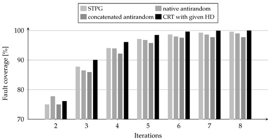
Figure 1.
Fault coverage comparison for different test generation methods for and (8 iterations).
In the next set of experiments, conducted in a simulation environment, the focus was on evaluating the effectiveness of test patterns generated using the proposed algorithm in detecting multicell RAM faults. Multicell memory faults, such as Pattern-Sensitive Faults (PSFs), involve dependencies between any k out of N memory cells (N being the memory size). These faults are triggered when specific binary patterns are present in the related cells or when particular transitions occur based on predefined conditions. Consequently, effective detection of such faults requires generating the largest possible number of binary patterns during testing. These patterns activate the faults and enable their detection.
The simulations analyzed groups consisting of k memory cells for . For each group, up to distinct k-bit binary patterns (i.e., values ranging from 0 to ) could potentially appear. The objective was to determine the average number of unique k-bit patterns generated during a march test, with the memory being initialized in each iteration using test patterns from the CRT with a given Hamming distance. The obtained results were compared with the results for random tests presented in Table 8.12 in [38].
Each simulation-based test consisted of a specific number of iterations, determined by the value of r: 4 iterations for , 8 iterations for , and 16 iterations for . During each iteration, the simulated memory was initialized with a given test pattern from the analyzed set, followed by the execution of a transparent version of the MATS+ memory test. Throughout the simulation, the memory model was monitored, and the number of unique k-bit binary patterns observed in individual groups of k-cells was recorded. The results are presented in Table 12.
Based on the results presented in Table 12, it can be concluded that CRTs consistently achieve better results than random tests in most cases. The difference is most noticeable for lower values of r and k, where the CRT outperforms random tests by several percentage points. For instance, for and , the CRT achieves a fault coverage of 97.27%, while random tests reach 93.74%. Fault coverage decreases as the value of k increases. This is expected, since the number of possible binary combinations grows exponentially, making full coverage harder to achieve. However, the results in Table 12 indicate that CRTs perform slightly better for larger k compared to random tests, highlighting the greater ability of a CRT to generate diverse test patterns.
In the final experiment, the average number of unique k-bit test patterns generated in arbitrary groups of k out of N memory cells using the proposed algorithm was compared with that obtained using traditional CRT generation methods, including native antirandom tests [13], concatenated antirandom tests [13], and STPG [40]. The comparison was carried out for fault groups of size , using tests generated for (i.e., 8 iterations). During the simulation, the number of distinct k-bit patterns generated in each iteration was recorded to assess the performance of the proposed method relative to the standard techniques. The outcomes of this analysis are presented in Figure 1, which illustrates the differences in the number of generated k-bit patterns across the tested methods.
The results show that the CRT method with a given Hamming distance consistently outperforms other test generation methods in terms of fault coverage, with one exception in the second iteration, where it achieves a slightly lower result (76.13%) compared to native antirandom (77.77%). However, starting from the third iteration, the CRT surpasses all other methods, demonstrating a faster increase in fault coverage (e.g., between iterations 2 and 3, the CRT rises from 76.13% to 90.05%). In the later iterations (7 and 8), the CRT approaches near-complete fault coverage, reaching 99.92% and 99.99%, respectively. Although the differences between the CRT and other methods diminish with a higher number of iterations, the CRT consistently demonstrates superior effectiveness, confirming its ability to generate diverse and efficient test patterns even in advanced stages of testing.
In summary, the experimental evaluation demonstrates that the proposed method consistently provides superior results compared to both purely random tests and classical controlled random tests. The improvements are systematic across all examined cases, particularly in terms of fault coverage and test diversity, while being achieved with significantly reduced computational effort.
6. Conclusions
This paper presented a method for generating controlled random tests with a given Hamming distance, aimed at improving the diversity and effectiveness of test sets used in computing systems, particularly memory devices. A new dissimilarity measure was introduced, based on Hamming distances calculated for binary patterns represented in various numeral systems. This extended measure allows for a more detailed assessment of differences between patterns compared to the classical Hamming distance alone.
We proposed an algorithm that generates test sets with a predefined minimum Hamming distance, without selecting patterns from large pools of candidates. This approach reduces computational effort while ensuring sufficient diversity in the generated patterns.
The effectiveness of the proposed method was evaluated through a series of comparative experiments. The results showed that the generated tests outperform not only purely random test sets but also traditional controlled random tests (CRTs) in several aspects. Specifically, tests created using the proposed method achieved higher total dissimilarity values and better coverage of multicell memory faults, particularly for lower numbers of iterations and smaller fault group sizes. Although some improvements observed in the experiments may appear moderate, they are systematic across all evaluated cases. More importantly, the obtained results demonstrate that these differences translate into tangible practical benefits, as the proposed method consistently achieves higher fault coverage than random and classical controlled random testing, especially in scenarios with smaller fault groups and lower iteration counts.
These results suggest that the method may be a practical alternative in contexts where test diversity and efficiency are important. Future work may include extending the approach to more complex fault models or exploring its use in different types of systems.
Author Contributions
Conceptualization, V.N.Y.; methodology, V.N.Y.; software, I.M.; validation, V.N.Y., I.M. and M.K.; formal analysis, V.N.Y. and I.M.; investigation, V.N.Y. and I.M.; writing—original draft preparation, V.N.Y. and I.M.; writing—review and editing, V.N.Y., I.M. and M.K. All authors have read and agreed to the published version of the manuscript.
Funding
This paper was supported by grant WZ/WI-ITI/3/2023 from the Faculty of Computer Science at Bialystok University of Technology, Ministry of Science and Higher Education, Poland.
Institutional Review Board Statement
Not applicable.
Informed Consent Statement
Not applicable.
Data Availability Statement
The original contributions presented in this study are included in the article. Further inquiries can be directed to the corresponding author.
Conflicts of Interest
The authors declare no conflicts of interest.
References
- Malaiya, Y.K.; Yang, S. The Coverage Problem for Random Testing. In Proceedings of the IEEE International Test Conference (ITC ’84), Philadelphia, PA, USA, 16–18 October 1984; pp. 237–245. [Google Scholar]
- Duran, J.W.; Ntafos, S.C. An Evaluation of Random Testing. IEEE Trans. Softw. Eng. 1984, 10, 438–444. [Google Scholar] [CrossRef]
- Arcuri, A.; Iqbal, M.Z.; Briand, L. Random Testing: Theoretical Results and Practical Implications. IEEE Trans. Softw. Eng. 2012, 38, 258–277. [Google Scholar] [CrossRef]
- Renfer, G. Automatic program testing. In Proceedings of the 3rd Conference of the Computing and Data Processing Society of Canada, Toronto, ON, USA, 2–3 June 1962. [Google Scholar]
- Anand, S.; Burke, E.K.; Chen, T.Y.; Clark, J.; Cohen, M.B.; Grieskamp, W.; Harman, M.; Harrold, M.J.; Mcminn, P. An Orchestrated Survey of Methodologies for Automated Software Test Case Generation. J. Syst. Softw. 2013, 86, 1978–2001. [Google Scholar] [CrossRef]
- Yarmolik, S.V.; Yarmolik, V.N. Controlled random tests. Autom. Remote Control 2012, 73, 1704–1714. [Google Scholar] [CrossRef]
- Huang, R.; Sun, W.; Xu, Y.; Chen, H.; Towey, D.; Xia, X. A survey on adaptive random testing. IEEE Trans. Softw. Eng. 2019, 47, 2052–2083. [Google Scholar] [CrossRef]
- Bardell, P.H.; McAnney, W.H.; Savir, J. Built-In Test for VLSI: Pseudorandom Techniques; John Wiley & Sons: New York, NY, USA, 1987. [Google Scholar]
- Das, D.; Karpovsky, M. Exhaustive and Near-Exhaustive Memory Testing Techniques and their BIST Implementations. J. Electron. Test. 1997, 10, 215–229. [Google Scholar] [CrossRef]
- McCluskey, E.J. Verification Testing—A Pseudoexhaustive Test Technique. IEEE Trans. Comput. 1984, C-33, 541–546. [Google Scholar] [CrossRef]
- Fujiwara, H. Logic Testing and Design for Testability; MIT Press: Cambridge, MA, USA, 1985. [Google Scholar] [CrossRef]
- Karpovsky, M.G.; van de Goor, A.J.; Yarmolik, V.N. Pseudo-Exhaustive Word-Oriented DRAM Testing. In Proceedings of the European Design and Test Conference (ED&TC), Paris, France, 6–9 March 1995; pp. 126–132. [Google Scholar] [CrossRef]
- Malaiya, Y.K. Antirandom Testing: Getting the Most out of Black-Box Testing. In Proceedings of the International Symposium on Software Reliability Engineering (ISSRE), Toulouse, France, 24–27 October 1995; pp. 86–95. [Google Scholar] [CrossRef]
- Wu, S.H.; Malaiya, Y.K.; Jayasumana, A.P. Antirandom vs. pseudorandom testing. In Proceedings of the IEEE International Conference on Computer Design: VLSI in Computers and Processors, Austin, TX, USA, 5–7 October 1998; p. 221. [Google Scholar]
- Wu, S.H.; Jandhyala, S.; Malaiya, Y.K.; Jayasumana, A.P. Antirandom Testing: A Distance-Based Approach. VLSI Des. 2008, 2008, 1–9. [Google Scholar] [CrossRef]
- Yin, H. Antirandom Test Patterns Generation Tool. In Technical Report CS-98-101; Computer Science Department, Colorado State University: Fort Collins, CO, USA, 1996; Fall 1996. [Google Scholar]
- von Mayrhauser, A.; Bai, A.; Chen, T.; Anderson, C.; Hajjar, A. Fast Antirandom (FAR) Test Generation. In Proceedings of the 3rd IEEE International Symposium on High-Assurance Systems Engineering, Washington, DC, USA, 13–14 November 1998; HASE ’98. pp. 262–269. [Google Scholar]
- Sahari, M.S.; A’ain, A.K.; Grout, I.A. Scalable Antirandom Testing (SAT). Int. J. Innov. Sci. Mod. Eng. 2015, 3, 33–35. [Google Scholar]
- Bodean, G.; Bodean, D.; Labunetz, A. New Schemes for Self-Testing RAM. In Proceedings of the Design, Automation and Test in Europe (DATE), Munich, Germany, 7–11 March 2005; Volume 2, pp. 858–859. [Google Scholar]
- Chen, T.Y.; Leung, H.; Mak, I.K. Adaptive Random Testing. In Proceedings of the 9th Asian Computing Science Conference, Chiang Mai, Thailand, 8–10 December 2004; pp. 320–329. [Google Scholar]
- Zhou, Z.Q. Using Coverage Information to Guide Test Case Selection in Adaptive Random Testing. In Proceedings of the 34th Annual IEEE Computer Software and Applications Conference Workshops (COMPSACW), Seoul, Republic of Korea, 19–23 July 2010; pp. 208–213. [Google Scholar] [CrossRef]
- Jiang, B.; Zhang, Z.; Chan, W.K.; Tse, T.H. Adaptive Random Test Case Prioritization. In Proceedings of the 24th IEEE/ACM International Conference on Automated Software Engineering (ASE), Auckland, New Zealand, 16–20 November 2009; pp. 233–244. [Google Scholar]
- Chan, K.P.; Chen, T.Y.; Towey, D. Good Random Testing. In Proceedings of the 9th Ada-Europe International Conference on Reliable Software Technologies, Palma de Mallorca, Spain, 14–18 June 2004; Llamosí, A., Strohmeier, A., Eds.; 2004; pp. 200–212. [Google Scholar] [CrossRef]
- Chan, K.P.; Chen, T.Y.; Towey, D. Restricted Random Testing. In Proceedings of the 7th European Conference on Software Quality, Helsinki, Finland, 9–13 June 2002; Kontio, J., Conradi, R., Eds.; pp. 321–330. [Google Scholar] [CrossRef]
- Chan, K.P.; Chen, T.Y.; Towey, D. Normalized Restricted Random Testing. In Lecture Notes in Computer Science, Proceedings of the 8th Ada-Europe International Conference on Reliable Software Technologies (Ada-Europe 2003), LNCS, Toulouse, France, 16–20 June 2003; Springer: Toulouse, France, 2003; Volume 2655, pp. 368–381. [Google Scholar] [CrossRef]
- Xu, S.; Chen, J. Maximum Distance Testing. In Proceedings of the Asian Test Symposium, Guam, GU, USA, 18–20 November 2002; pp. 15–20. [Google Scholar]
- Kuo, F. An Indepth Study of Mirror Adaptive Random Testing. In Proceedings of the Ninth International Conference on Quality Software, QSIC 2009, Jeju, Republic of Korea, 24–25 August 2009; Choi, B., Ed.; IEEE Computer Society: Washington, DC, USA, 2009; pp. 51–58. [Google Scholar]
- Xu, S. Orderly Random Testing for Both Hardware and Software. In Proceedings of the 14th IEEE Pacific Rim International Symposium on Dependable Computing, Washington, DC, USA, 15–17 December 2008; pp. 160–167. [Google Scholar]
- Nikravan, E.; Parsa, S. Hybrid adaptive random testing. Int. J. Comput. Sci. Math. 2020, 11, 209–221. [Google Scholar] [CrossRef][Green Version]
- Tappenden, A.; Miller, J. A Novel Evolutionary Approach for Adaptive Random Testing. IEEE Trans. Reliab. 2009, 58, 619–633. [Google Scholar] [CrossRef]
- Grindal, M.; Offutt, J.; Andler, S.F. Combination Testing Strategies—A Survey; Technical Report ISE-TR-04-05, GMU Technical Report; George Mason University: Fairfax, VA, USA, 2004. [Google Scholar]
- Chen, T.Y.; Kuo, F.C.; Merkel, R.G.; Tse, T.H. Adaptive Random Testing: The ART of test case diversity. J. Syst. Softw. 2010, 83, 60–66. [Google Scholar] [CrossRef]
- Feldt, R.; Poulding, S.; Clark, D.; Yoo, S. Test Set Diameter: Quantifying the Diversity of Sets of Test Cases. In Proceedings of the IEEE International Conference on Software Testing, Verification and Validation (ICST), Chicago, IL, USA, 11–15 April 2016; pp. 223–233. [Google Scholar] [CrossRef]
- Arcuri, A.; Briand, L.C. Adaptive random testing: An illusion of effectiveness? In Proceedings of the 20th International Symposium on Software Testing and Analysis (ISSTA 2011), Toronto, ON, Canada, 17–21 July 2011; pp. 265–275. [Google Scholar] [CrossRef]
- Hamming, R.W. Error detecting and error correcting codes. Bell Syst. Tech. J. 1950, 29, 147–160. [Google Scholar] [CrossRef]
- Peterson, W.W.; Weldon, E.J. Error-Correcting Codes, 2nd ed.; MIT Press: Cambridge, MA, USA, 1972. [Google Scholar]
- Plotkin, M. Binary codes with specified minimum distance. IIRE Trans. Inf. Theory 1960, 6, 445–450. [Google Scholar] [CrossRef]
- Mrozek, I. Multi-Run Memory Tests for Pattern Sensitive Faults; Springer International Publishing: Cham, Switzerland, 2019. [Google Scholar] [CrossRef]
- Mrozek, I.; Yarmolik, V.N. Optimal Controlled Random Tests. In Proceedings of the Computer Information Systems and Industrial Management: 16th IFIP TC8 International Conference, CISIM 2017, Białystok, Poland, 16–18 June 2017; Lecture Notes in Computer Science; Springer: Berlin/Heidelberg, Germany, 2017; Volume 10244, pp. 27–38. [Google Scholar] [CrossRef]
- Yiunn, D.B.Y.; Bin A’ain, A.K.; Khor Ghee, J. Scalable test pattern generation (STPG). In Proceedings of the IEEE Symposium on Industrial Electronics Applications (ISIEA ’10), Penang, Malaysia, 3–5 October 2010; pp. 433–435. [Google Scholar] [CrossRef]

Disclaimer/Publisher’s Note: The statements, opinions and data contained in all publications are solely those of the individual author(s) and contributor(s) and not of MDPI and/or the editor(s). MDPI and/or the editor(s) disclaim responsibility for any injury to people or property resulting from any ideas, methods, instructions or products referred to in the content. |
© 2025 by the authors. Licensee MDPI, Basel, Switzerland. This article is an open access article distributed under the terms and conditions of the Creative Commons Attribution (CC BY) license (https://creativecommons.org/licenses/by/4.0/).