Dynamic Load Analysis of Vertical, Pitching, and Lateral Tilt Vibrations of Multi-Axle Vehicles

Featured Application

The study systematically analyzes the dynamic loads generated by multi-axle vehicles during vertical, pitching, and lateral tilt vibrations, revealing their mechanisms of action on pavement structures. The research findings can be effectively applied to pavement design and lifecycle performance evaluation, helping engineering professionals to better understand the mechanisms by which vehicle-induced dynamic loads lead to pavement deformation, fatigue damage, and long-term performance degradation. It serves as a theoretical foundation for improving the durability and service performance of road infrastructure.

Abstract

The dynamic load caused by vehicle vibration due to an uneven pavement surface is a primary factor affecting the structural performance and service life of asphalt pavement. As the principles of vibration mechanics, in conjunction with the coherence function of the vehicle’s left and right wheels, along with the lag between front and rear wheels, the entire vehicle vibration model for three-axle and four-axle heavy-load vehicles was developed using Simulink software. Through simulation, the root-mean-square value of the dynamic load and the dynamic load coefficient of the vehicle with different pavement roughness grades, speeds, loads, and cornering radii were analyzed. The outcomes demonstrate that a nonlinear rise in the wheel dynamic load occurs when pavement roughness increases. The greater the speed, the greater the impact of pavement roughness on the dynamic load. An increase in vehicle load tends to reduce vehicle vibrations. The interaction between vehicle vibration frequency and road excitation frequency is essential in figuring out the loads, and a negative influence on the pavement structure should be given more attention when the vehicle is driving at low speed. The dynamic load coefficient of the left and right wheels is greatly affected when the vehicle is in a lateral tilt. The findings offer valuable insights for selecting appropriate loads in pavement structure design. By constructing 11 degrees of freedom for a three-axle vehicle and 16 degrees of freedom for a four-axle heavy-duty vehicle model, the dynamic load variation law under different roughness excitation conditions is systematically analyzed. The results can be applied to the selection of vehicle load in asphalt pavement design to make it closer to the actual driving state, which will be helpful for improving accuracy in the design of pavement structure and avoiding early damage to the pavement.

1. Introduction

Due to the rapid growth of highway transportation, especially the trend of high-speed vehicles and heavy-load vehicles, the destruction of asphalt pavement is a common occurrence. The method for designing asphalt pavement in China simplifies the vehicle load into a double-circle vertical uniform static load and ignores the effect of the loads of the vehicle; static mode analysis leads to a large difference from the real stress condition of the pavement structure [1]. Therefore, it is essential to analyze the dynamic load due to vehicle vibrations.

An uneven pavement surface is a primary cause of the loading effects of vehicles. The LTTP project study in the USA showed that pavement performance is significantly connected to roughness when construction is completed. Dodds [2] found that pavement surface roughness is the primary source of vehicle vibration. Cebon [3] found that the dynamic load frequency is generally 1~15 Hz and suggested that a key factor in pavement surface damage is the interaction between vehicles and the pavement. Watts [4] concluded that the vibration generated by the vehicle is associated with the degree to which the pavement surface roughness is dispersed. Deng [5] proposed that the roughness of the pavement has a Gaussian stationarity characteristic with a zero mean.

For the vibratory loading of the vehicle, simulation typically employs a vehicle vibration model subjected to pavement surface excitation, along with the dynamic load coefficient [6], and other indicators are obtained to describe it. There are also some direct measurement methods, such as Mitschke [7], whereby the load data are read directly by pre-installed dynamic load test sensors on the field test vehicle. Chen [8] backward-deduced the vibration load of the vehicle by measuring the accelerated speed values at different points of the sprung and unsprung systems of the vehicle. However, the above method is expensive, and the experimental findings depend on the precision of the sensors.

For vehicle modeling, numerical simulation technology is usually used to simplify the vehicle into a parametric model featuring a limited number of degrees of freedom, and the vibration theory is used to solve the dynamic load. Sun [9] used the one-quarter vehicle model and the half-vehicle model to analyze the loading effects of vehicles at different speeds by using the state-space method and the transfer function method, respectively, and showed that the vibratory loading coefficient of the vehicle showed an opposite trend during the period of acceleration and deceleration. Sayers [10] analyzed the effects of the suspension system, acceleration and deceleration, the pavement surface roughness, and the tire damping and stiffness coefficients on vibratory loading and pavement performance by establishing a half-vehicle model, and found that the vertical pressure of a single wheel on the pavement is greater than that of a double wheel set. Zhong [11] established a two-degree-of-freedom vehicle model and used measured power spectral density of pavement roughness as an external excitation input to analyze the pavement surface’s unpredictable loads during vehicle driving. Tao [12] used the traditional two-degree-of-freedom vehicle model to establish the system vibration equation, and used the frequency domain technique to describe characteristics and variation laws of the dynamic load. Tan [13] established and simulated a time-domain model of one-quarter vehicle excitation by determining the parameters of the rational function power spectrum. Jin [14] used ADAMS software to build a vehicle model and modeled the vehicle’s nonlinear random vibration response. Xie [15] used the three-axle half-vehicle and four-axle half-vehicle models with a balanced suspension structure to calculate the variation in the vehicle’s vibration motion and examined the impact of different pavement conditions and driving conditions on the vehicle’s dynamic load, but they only considered the vehicle’s vertical and pitching motion. Beskou et al. [16] proposed a unified finite element processing method for three-dimensional flexible pavement, which realized the leap from two-dimensional to three-dimensional analysis. Si [17] performed random vibration analysis of linear continuous systems under moving random loads, which provides a theoretical basis for complex system modeling. Lv [18] systematically analyzed asphalt pavement’s stress and strain under arbitrary loads, which transcended the traditional single index evaluation.

The unevenness of the pavement surface causes the vehicle to generate vibratory loading, and simultaneously, the dynamic load reacts upon the pavement surface. Therefore, some scholars have researched vehicle pavement system interactions. For example, Mamlouk [19] and FRÝBA [20] found that the loads of the vehicle in motion increased on an uneven pavement surface, and a surge in dynamic load worsens the pavement’s surface roughness, so the concept of coupling the vehicle and pavement surface was proposed. Deng [5] regarded the pavement structure layer and the vehicle as a whole system, and described the effect of pavement roughness excitation on the wheels. Liang [21] established an overall model of two subsystems, including the one-quarter vehicle model and the discrete finite element of pavement structure, regarded the vehicle and pavement as an interactive whole, and iteratively solved the dynamic balancing equation of the vehicle pavement coupling system using the N-R and Newmark-β methods. Li [22] established a system for the interaction between vehicles, the pavement surface, and subgrade and examined how surface and vehicle characteristics affected the random loads of vehicles using an eight-degree-of-freedom vehicle model. Zhao [23] used the filtered white noise method to establish the road excitation model and constructed a more realistic vehicle vibration simulation model. Dong & Ma [24] specifically analyzed the response of asphalt pavement under non-uniform tire contact pressure and an irregular tire imprint, demonstrating that researchers were beginning to pay attention to the fine characteristics of tire–pavement contact. The latest research by Zeng et al. [25] introduces vibro-acoustic analysis into the field of road dynamics, creating a new dimension for studying vehicle road interactions. The research of Mo [26] shows that the current research has not only focused on the road response, but also considered vehicle comfort, which reflects the two-way expansion of the research perspective. In the literature of topology optimization of bogie frames [27] and lightweight design of carboy under multi-axis random load [28]: studies have examined the structural behavior and dynamic response of railway bogie frames under vibration and multi-axle interaction conditions, emphasizing how bogie design influences vehicle stability and load distribution. Through the dynamic optimization method, it is shown how the body design affects the overall vibration behavior and dynamic load transfer, and a valuable comparison framework is provided. Although the contact conditions of highway and railway systems are different, the quantitative methods of multi-axis load transfer and vibration fatigue are directly related to this work.

From the above research, it is evident that the one-quarter model or the half-vehicle model is generally selected, which means that the lateral tilt vibration caused by the left and right wheels of the vehicle is ignored, but driving trajectory of left and right wheels of the vehicle cannot be exactly the same; additionally, for the pavement surface excitation for the left and right wheels, lateral tilt vibration cannot be ignored. There are thus obvious shortcomings in the use of single-wheel and half-vehicle models. At the same time, most of the studies focus on the simulation analysis of two-axle vehicles, but multi-axle heavy-duty vehicles have become an important model of highway transportation in China, and the influence between each wheel and axle is more complex than that of two-axle vehicles due to the increase in axle count.

Based on the existing relevant research, in this study, the excitation of the pavement surface is taken as the influence factor, a pavement excitation model is established using the filtered white noise method; a vibration model of the three-axle and four-axle heavy-duty vehicles with a balanced suspension structure, including vertical, pitch, and lateral tilt vibrations, is established; the variation law of the random dynamic load of the multi-axle vehicle is analyzed through simulation; the impact of varying the working conditions (vehicle speed, road roughness, and vehicle load) on the random dynamic load of the vehicle is analyzed. To give the vehicle load utilized in asphalt pavement design a more precise theoretical foundation, the design model can more accurately reflect actual traffic load characteristics. The research in this paper provides a new and more comprehensive perspective for understanding the failure mechanism of heavy-duty vehicles on pavement from the analysis gap in the key link from ‘vehicle complex vibration’ to ‘dynamic load output’.

2. Pavement Roughness Excitation Model

2.1. Pavement Roughness Excitation Power Spectral Density

The distribution of energy in randomly varying pavement heights at different frequencies is explained by the power spectral density (PSD) of pavement roughness. It is a frequency domain analysis tool used to describe pavement roughness, typically expressed as the relationship between the variance and frequency of pavement height per unit distance or unit length. Numerous measured outcomes demonstrate that the frequency of pavement roughness amplitude has different characteristics in different road sections. Therefore, mathematically, a zero-mean stationary Gaussian random process in each state can be thought of as the road profile roughness sequence, PSD can be applied to characterize its statistical characteristics [29], and the expression is

$$G_q\left(n\right)=G_q\left(n_0\right){\left({\displaystyle \frac{n}{n_0}}\right)}^{-\omega },n>0$$

(1)

where n is the geographic frequency, which is the reciprocal of the wavelength, m⁻¹; n₀ is the reference spatial frequency, whose value is 0.1; G_q(n₀) is the pavement roughness coefficient; m³. ω is the frequency coefficient, whose value is two.

Pavement roughness can be classified into eight levels [30], as displayed in

Table 1. Pavement roughness grading criteria.

Pavement Grade	$\mathbf{Power}\mathbf{Spectral}\mathbf{Density}{\mathit{G}}_{\mathit{d}}\left({\mathit{n}}_0\right)/{10}^{-6}{\mathbf{m}}^3$
	Lower Limit	Geometric Mean	Upper Limit
A	8	16	32
B	32	64	128
C	128	256	512
D	512	1024	2048
E	2048	4096	8192
F	8192	16,384	32,768
G	32,768	65,536	131,072
H	131,072	262,144	524,288

.

2.2. Time-Domain Pavement Excitation Model Using the Filtered White Noise Technique

• Time-domain model of single-wheel pavement excitation

The single-wheel pavement excitation $q\left(t\right)$ is regarded by the filtered white noise method as a first-order linear system of white noise excitation $\omega \left(t\right)$. The system’s frequency response function, taking into account the pavement’s cut-off frequency, is

$$H_{q-\omega }\left(\omega \right)={\displaystyle \frac{2\pi n_0\sqrt{G_q\left(n_0\right)u}}{j\omega +{\omega }_0}}$$

(2)

where: ω is the circular frequency, rad/s, $\omega$ = 2$\pi un$; u is the vehicle speed, m/s.

Changing Equation (2) to a differential equation expression, the time-domain model of the single-wheel pavement excitation is

$$q^{\prime }\left(t\right)=-2\pi f_0\cdot q\left(t\right)+2\pi n_0\sqrt{G_q\left(n_0\right)u}\cdot \omega \left(t\right)$$

(3)

By substituting different vehicle speeds u, the pavement’s time-domain model at each vehicle speed can be obtained. Still, there is some discrepancy between the conclusions of the model and the real pavement conditions, because the cut-off frequency under the actual pavement roughness should be the spatial frequency, not the time frequency. The time-domain model of the filtered white noise pavement roughness should be as follows, since the lower cut-off time frequency may be derived from the lower cut-off spatial frequency and vehicle speed:

$$q^{\prime }\left(t\right)=-2\pi n_{00}u\cdot q\left(t\right)+2\pi n_0\sqrt{G_q\left(n_0\right)u}\cdot \omega \left(t\right)$$

(4)

where n₀₀ is the lower cut-off spatial frequency of pavement roughness, n₀₀ = 0.01 m⁻¹.

2.

The coherence function of the left and right wheels

Statistical characteristics of pavement surface roughness are described by the respective power spectral density functions of the left and right wheels and their mutual power spectral density functions or coherence functions. A coherent function is defined as

$$co{h}_{LR}^2\left(\omega \right)={\displaystyle \frac{{\left|G_{LR}\left(\omega \right)\right|}^2}{G_{LL}\left(\omega \right)G_{RR}\left(\omega \right)}}$$

(5)

where, $G_{xy}\left(\omega \right)$ is the cross-spectrum of the left and right wheel track pavement input; $G_{LL}\left(\omega \right)$ is the self-spectrum of the left wheel track pavement input; $G_{RR}\left(\omega \right)$ is the self-spectrum of the right wheel track pavement input. The parametric model proposed by Robson [31] is usually used:

$$co{h}_{LR}\left(\omega \right)=e^{-{\displaystyle \frac{B}{u}}\omega }$$

(6)

where B is the vehicle’s wheel span, m; u is the vehicle’s speed, m/s.

3.

The time-domain relationship of left and right wheel pavement excitation

Using the time-domain model of Equation (4), the left and right wheel track $x\left(t\right)$ and $y\left(t\right)$ can be generated from the white noise excitation ${\omega }_x\left(t\right)$ and ${\omega }_y\left(t\right)$, respectively, and the statistical characteristics of both are the same, that is,

$$G_x\left(\omega \right)=G_y\left(\omega \right)$$

(7)

Suppose that the frequency response function of the system output ${\omega }_y\left(t\right)$ and input ${\omega }_x\left(t\right)$, are $H_1\left(\omega \right)$; that is,

$$W_y\left(\omega \right)=H_1\left(\omega \right)W_x\left(\omega \right)$$

(8)

According to random vibration theory, the following expression represents the relationship between the left wheel’s auto-power spectral density and the cross-power spectral densities of the left and right wheels:

$$G_{xy}\left(\omega \right)=H_1\left(\omega \right)G_{xx}\left(\omega \right)$$

(9)

From Equation (5) to Equation (8), the frequency response function, $H_1\left(\omega \right)$, and the coherence function are equal; that is,

$$H_1\left(\omega \right)=co{h}_{LR}\left(\omega \right)$$

(10)

Subsequently, the relationship involving the auto-power spectral density of white noise ${\omega }_y\left(t\right)$ of incoherent white noise and self-power spectral density ${\omega }_y\left(t\right)$ is as follows:

$$H_1\left(\omega \right)={\displaystyle \frac{G_{\omega y}\left(\omega \right)}{G_{\omega x}\left(\omega \right)}}={\displaystyle \frac{a_0+a_{1}s+a_2{s}^2}{b_0+b_{1}s+b_2{s}^2}}$$

(11)

Take the intermediate variable $M\left(s\right)$, and multiply the numerator and denominator together, $s^{-2}M\left(s\right)$; that is,

$${\displaystyle \frac{G_{\omega y}\left(\omega \right)}{G_{\omega x}\left(\omega \right)}}={\displaystyle \frac{\left(a_0{s}^{-2}+a_1{s}^{-1}+a_2\right)M\left(s\right)}{\left(b_0{s}^{-2}+b_1{s}^{-1}+b_2\right)M\left(s\right)}}$$

(12)

Detach Equation (12) from the numerator and denominator, and obtain [32] by shifting the term:

$$\left\{\begin{array}{c}M\left(s\right)=-{\displaystyle \frac{a_0}{a_2}}{s}^{-2}M\left(s\right)-{\displaystyle \frac{a_1}{a_2}}{s}^{-1}M\left(s\right)+{\displaystyle \frac{1}{a_2}}{G}_{\omega y}\left(\omega \right)\\ M\left(s\right)=-{\displaystyle \frac{b_0}{b_2}}{s}^{-2}M\left(s\right)-{\displaystyle \frac{b_1}{b_2}}{s}^{-1}M\left(s\right)+{\displaystyle \frac{1}{b_2}}{G}_{\omega x}\left(\omega \right)\end{array}\right.$$

(13)

Let $x_1=L^{-1}\left[s^{-1}M\left(s\right)\right]$ and $x_3=L^{-1}\left[s^{-2}M\left(s\right)\right]$; thereinto, $L^{-1}\left[s^{-2}M\left(s\right)\right]$ represents the Laplace inverse transformation; ${\dot{x}}_3=x_1$; ${\dot{x}}_3=m\left(t\right)$; $m\left(t\right)$ is the Laplace inverse transformation of $M\left(s\right)$; then,

$$\left\{\begin{array}{c}{\dot{x}}_1=-{\displaystyle \frac{a_0}{a_2}}{x}_3-{\displaystyle \frac{a_1}{a_2}}{x}_1+{\displaystyle \frac{1}{a_2}}{q}_2\\ {\dot{x}}_3=-{\displaystyle \frac{b_0}{b_2}}{x}_3-{\displaystyle \frac{b_1}{b_2}}{x}_1+{\displaystyle \frac{1}{b_2}}{q}_1\end{array}\right.$$

(14)

The equation above provides the spatial space expression:

$$\left\{\begin{array}{c}\left[\begin{array}{c}{\dot{x}}_1\\ {\dot{x}}_3\end{array}\right]=\left[\begin{array}{cc}-{\displaystyle \frac{b_1}{b_2}}& -{\displaystyle \frac{b_0}{b_2}}\\ 1& 0\end{array}\right]\left[\begin{array}{c}{x}_1\\ x_3\end{array}\right]+\left[\begin{array}{c}{\displaystyle \frac{1}{b_2}}\\ 0\end{array}\right]q_1\\ q_3=\left[\begin{array}{cc}{a}_1-a_2{\displaystyle \frac{b_1}{b_2}}& a_0-a_2{\displaystyle \frac{b_0}{b_2}}\end{array}\right]\left[\begin{array}{c}{x}_1\\ x_3\end{array}\right]+\left[{\displaystyle \frac{a_2}{b_2}}\right]q_1\\ {\dot{q}}_3={\left[\begin{array}{c}{c}_{31}\\ c_{32}\end{array}\right]}^T\left[\begin{array}{c}{x}_1\\ x_3\end{array}\right]+\left[{\displaystyle \frac{a_1}{b_2}}-{\displaystyle \frac{a_2{b}_1}{b_2^2}}\right]q_1+\left[{\displaystyle \frac{a_2}{b_2}}\right]{\dot{q}}_1\\ \begin{array}{c}{c}_{31}={\displaystyle \frac{a_2{b}_1^2}{b_2^2}}-{\displaystyle \frac{a_1{b}_1+a_2{b}_0}{b_2}}+a_0\\ c_{32}={\displaystyle \frac{a_2{b}_0{b}_1}{b_2^2}}-{\displaystyle \frac{a_1{b}_0}{b_2}}\end{array}\end{array}\right.$$

(15)

The undetermined coefficients in Equation (15) can be obtained by the optimization algorithm [33], where the objective function and constraints are

$$\left\{\begin{array}{c}Q=\mathit{min}{\sum }_1^n\left|\left|{\displaystyle \frac{a_0+a_1\left(j{\omega }_i\right)-a_2{\omega }_i^2}{b_0+b_1\left(j{\omega }_i\right)-b_2{\omega }_i^2}}\right|-e^{{\displaystyle \frac{-{\omega }_{i}B}{u}}}\right|\\ \left|\left|{\displaystyle \frac{a_0+a_1\left(j{\omega }_i\right)-a_2{\omega }_i^2}{b_0+b_1\left(j{\omega }_i\right)-b_2{\omega }_i^2}}\right|-e^{{\displaystyle \frac{-{\omega }_{i}B}{u}}}\right|<\mu \end{array}\right.$$

(16)

where ${\omega }_i$ is the angular frequency of optimization, ${\omega }_i=\mathrm{0,0.5},...;i=\mathrm{1,2},...,n$; μ is a small positive number. $a_0\sim b_2$ are the variables; they are related to the vehicle speed u, wheel span B, and pavement surface roughness coefficient, $G_q\left(n_0\right)$.

4.

The time-domain relationship of front and rear wheel pavement excitation

When traveling at a steady speed, the rear wheel’s pavement excitation on the same side temporarily lags behind the front wheel, T:

$$T=L/u$$

(17)

Next, the connection between the front and rear wheel pavement excitation [34] is

$$q_r\left(t\right)=q_f\left(t-{\rm T}\right)$$

(18)

where L is the wheelbase of the vehicle, m; $q_r\left(t\right)\mathrm{a}\mathrm{n}\mathrm{d};q_f\left(t\right)$are the pavement excitation of the front and rear wheels on the same side, respectively.

2.3. Simulation of Time-Domain Pavement Excitation for Filtered White Noise

Simulink software (2020 version) was used to create a time-domain simulation model of pavement excitation. During the simulation, according to the different values of $G_q\left(n_0\right)$, u, B, and L, the excitation time-domain curves of the pavement under different working conditions can be obtained.

Take the pavement roughness of grade B as an example, that is, the pavement roughness coefficient, $G_q\left(n_0\right)=64\times 10^{-6}{\mathrm{m}}^3$, and then assume that the vehicle speed u = 25 m/s, wheelbase L = 6.2 m, wheel span B = 3 m, and simulation time 8 s; the simulation outcomes are presented in Figure 1.

Differences in the pavement excitation time-domain curves of the left and right front axle wheels are shown in Figure 1, attributed to the coherence function. On the other hand, the left and right rear axle wheels have a time lag with their respective front axle wheels, so the corresponding straight line is zero at the beginning of the figure. In subsequent studies, the model was used as a pavement input for vehicle model simulation.

3. Simplified Vibration Model of Vehicle System

The vehicle is a “spring mass damping” drive system composed of multiple degrees of freedom, including a suspension, an engine, wheels, a body, and other subsystems, and each subsystem is connected to the other with damping elements and hinges, so the vehicle system is very complex. When performing vehicle vibration analysis, it is common to simplify the vehicle model. At present, commonly used simplified models include a two-degree-of-freedom single-wheel model, a four-degree-of-freedom half-vehicle model, a seven-degree-of-freedom whole vehicle model, etc.

The two-degree-of-freedom single-wheel model only considers vertical vibration of the vehicle in motion. The four-degree-of-freedom half-vehicle model assumes that the vehicle is symmetrical along the longitudinal axle; the excitation function of the left and right wheels is the same, and it has four degrees of freedom, such as the body’s pitch and vertical vibrations, and vertical runout of the front and rear wheels. In reality, the vehicle is not completely symmetrical, and the pavement surface under each wheel during driving cannot be completely consistent, such that the impact of surface conditions and vehicle attributes on the vehicle can be more accurately reflected in a whole-vehicle model. The simplest three-dimensional whole-vehicle model is the seven-degree-of-freedom model, which builds upon the half-vehicle model by including the vehicle’s lateral roll movement and the vertical movement of the wheels on the opposite side of the body, for a total of seven degrees of freedom.

The results of the traffic survey show that the majority of vehicles are three-axle vehicles with a load of more than 10 t, and four-axle semi-trailer vehicles account for the largest proportion among the trailers. Therefore, the analysis is conducted based on vehicle vibration models established for two types of vehicles: three-axle and four-axle vehicles.

3.1. Whole-Vehicle Model of Three-Axle Vehicle

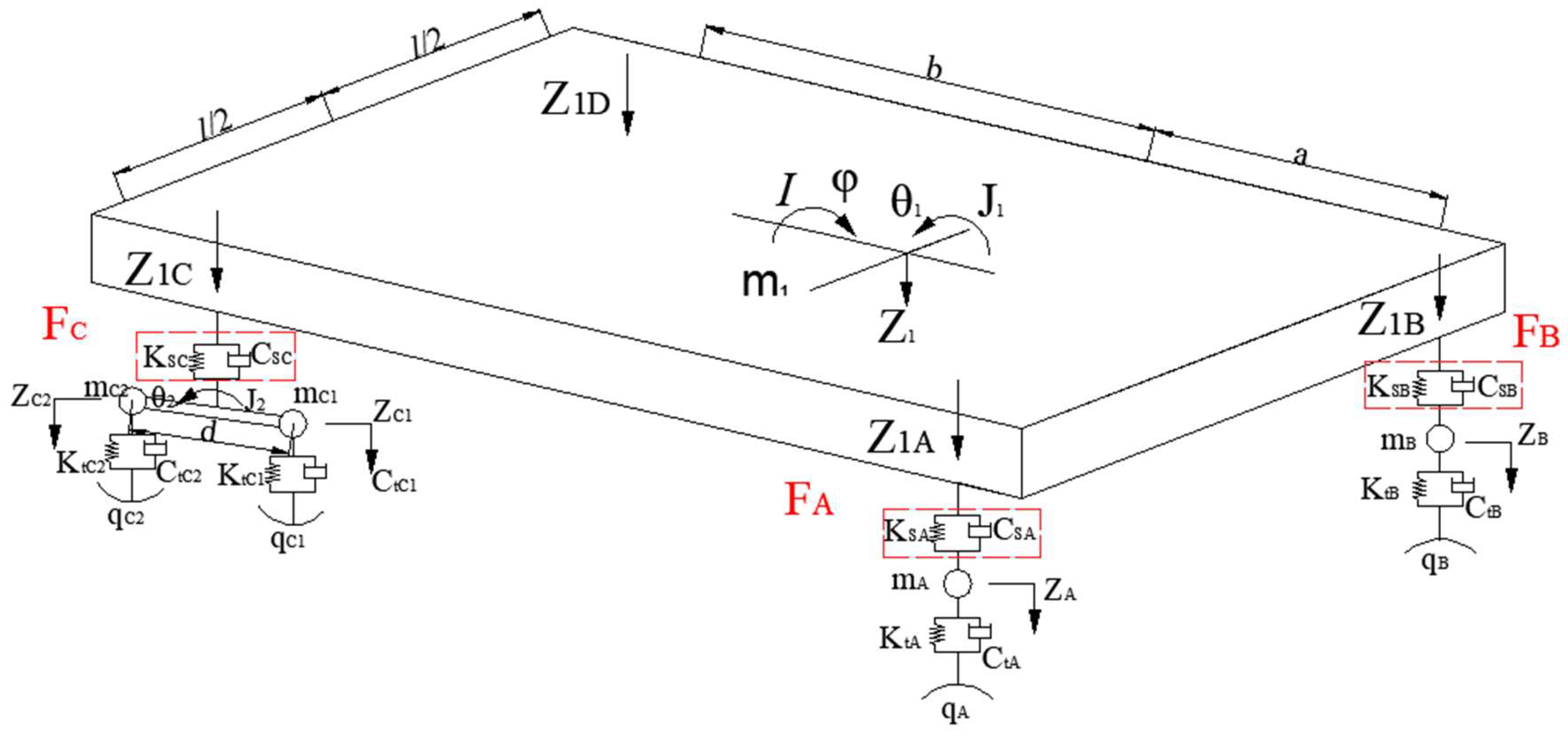
After appropriate simplification, a model with 11 degrees of freedom for a three-axle vehicle can be established and simplified into a centralized mass, spring, and damping model, as depicted in Figure 2.

In the model, A and B are the left and right wheels of the front axle, C1 and D1 are the left and right wheels of the intermediate shaft, and C2 and D2 are the left and right wheels of the rear axle. The degrees of freedom comprise 3 for body pitch, vertical, and roll, 2 for rear balance-suspension pitch, and 6 for the vertical motion of the front axle, intermediate shaft, and rear axles, totaling 11.

With the front-axle wheel taken as an example, the single-wheel model consists of tire stiffness K, tire damping Ct, suspension stiffness Ks, suspension damping Cs, and unsprung mass m; pavement contact is described by the roughness excitation q.

The vehicle model’s second-order vibrational differential equation is as follows, in accordance with Newton’s second law:

The vertical vibration of the body:

$$m_1{z}_1^{\prime \prime }=F_A+F_B+F_C+F_D$$

(19)

The pitching vibration of the body:

$$J_1{\theta }_1^{\prime \prime }=b\left(F_C+F_D\right)-a\left(F_A+F_B\right)$$

(20)

Lateral tilt vibration of the body:

$$I{\phi }^{\prime \prime }={\displaystyle \frac{l}{2}}\left[F_B+F_D-F_A-F_C\right]$$

(21)

Pitching vibration of rear balance suspension:

$$J_2{\theta }_2^{\prime \prime }={\displaystyle \frac{1}{2}}d\left[k_{t{C}_2}\left(q_{C_2}-z_{C_2}\right)-c_{t{C}_2}\left(q_{C_2}^{\prime }-z_{C_2}^{\prime }\right)\right]-{\displaystyle \frac{1}{2}}d\left[k_{t{C}_1}\left(q_{C_1}-z_{C_1}\right)-c_{t{C}_1}\left(q_{C_1}^{\prime }-z_{C_1}^{\prime }\right)\right]$$

(22)

$$J_3{\theta }_3^{\prime \prime }={\displaystyle \frac{1}{2}}d\left[k_{t{D}_2}\left(q_{D_2}-z_{D_2}\right)-c_{t{D}_2}\left(q_{D_2}^{\prime }-z_{D_2}^{\prime }\right)\right]-{\displaystyle \frac{1}{2}}d\left[k_{t{D}_1}\left(q_{D_1}-z_{D_1}\right)-c_{t{D}_1}\left(q_{D_1}^{\prime }-z_{D_1}^{\prime }\right)\right]$$

(23)

Vertical vibration of the front axle wheels:

$$m_A{z}_A^{\prime \prime }=k_{tA}\left(q_A-z_A\right)+c_{tA}\left(q_A^{\prime }-z_A^{\prime }\right)-F_A$$

(24)

$$m_B{z}_B^{\prime \prime }=k_{tB}\left(q_B-z_B\right)+c_{tB}\left(q_B^{\prime }-z_B^{\prime }\right)-F_B$$

(25)

Vertical vibration of the rear axle wheels:

$$m_{C_1}{z}_{C_1}^{\prime \prime }=k_{t{C}_1}\left(q_{C_1}-z_{C_1}\right)+c_{t{C}_1}\left(q_{C_1}^{\prime }-z_{C_1}^{\prime }\right)-{\displaystyle \frac{1}{2}}{F}_C$$

(26)

$$m_{C_2}{z}_{C_2}^{\prime \prime }=k_{t{C}_2}\left(q_{C_2}-z_{C_2}\right)+c_{t{C}_2}\left(q_{C_2}^{\prime }-z_{C_2}^{\prime }\right)-{\displaystyle \frac{1}{2}}{F}_C$$

(27)

$$m_{D_1}{z}_{D_1}^{\prime \prime }=k_{t{D}_1}\left(q_{D_1}-z_{D_1}\right)+c_{t{D}_1}\left(q_{D_1}^{\prime }-z_{D_1}^{\prime }\right)-{\displaystyle \frac{1}{2}}{F}_D$$

(28)

$$m_{D_2}{z}_{D_2}^{\prime \prime }=k_{t{D}_2}\left(q_{D_2}-z_{D_2}\right)+c_{t{D}_2}\left(q_{D_2}^{\prime }-z_{D_2}^{\prime }\right)-{\displaystyle \frac{1}{2}}{F}_D$$

(29)

F_A; F_B; F_C; F_D are the forces of each suspension, and their expressions are

$$F_A=k_{sA}\left(z_A-z_{1A}\right)+c_{sA}\left(z_A^{\prime }-z_{1A}^{\prime }\right)$$

(30)

$$F_B=k_{sB}\left(z_B-z_{1B}\right)+c_{sB}\left(z_B^{\prime }-z_{1B}^{\prime }\right)$$

(31)

$$F_C=k_{sC}\left[{\displaystyle \frac{1}{2}}\left(z_{C1}+z_{C2}\right)-z_{1C}\right]+c_{sC}\left[{\displaystyle \frac{1}{2}}\left(z_{C1}^{\prime }+z_{C2}^{\prime }\right)-z_{1C}^{\prime }\right]$$

(32)

$$F_D=k_{sD}\left[{\displaystyle \frac{1}{2}}\left(z_{D1}+z_{D2}\right)-z_{1D}\right]+c_{sD}\left[{\displaystyle \frac{1}{2}}\left(z_{D1}^{\prime }+z_{D2}^{\prime }\right)-z_{1D}^{\prime }\right]$$

(33)

Because the pitching angle θ and the lateral tilt angle φ values in the model are generally small, there are sin θ ≈ θ, sin φ ≈ φ, so the following relationship holds:

$$z_{1A}=z_1-a\mathit{sin}{\theta }_1-{\displaystyle \frac{1}{2}}l\mathit{sin}\phi =z_1-a{\theta }_1-{\displaystyle \frac{1}{2}}l\phi$$

(34)

$$z_{1B}=z_1-a\mathit{sin}{\theta }_1+{\displaystyle \frac{1}{2}}l\mathit{sin}\phi =z_1-a{\theta }_1+{\displaystyle \frac{1}{2}}l\phi$$

(35)

$$z_{1C}=z_1+b\mathit{sin}{\theta }_1-{\displaystyle \frac{1}{2}}l\mathit{sin}\phi =z_1+b{\theta }_1-{\displaystyle \frac{1}{2}}l\phi$$

(36)

$$z_{1D}=z_1+b\mathit{sin}{\theta }_1+{\displaystyle \frac{1}{2}}l\mathit{sin}\phi =z_1+b{\theta }_1+{\displaystyle \frac{1}{2}}l\phi$$

(37)

The expression of the vibratory loading of each wheel can be obtained:

Vibratory loading of the front wheels:

$$\left\{\begin{array}{c}{F}_1\left(t\right)=k_{tA}\left(q_A-z_A\right)+c_{tA}\left(q_A^{\prime }-z_A^{\prime }\right)\\ F_2\left(t\right)=k_{tB}\left(q_B-z_B\right)+c_{tB}\left(q_B^{\prime }-z_B^{\prime }\right)\end{array}\right.$$

(38)

Dynamic load of the intermediate wheels:

$$\left\{\begin{array}{c}{F}_3\left(t\right)=k_{t{C}_1}\left(q_{C_1}-z_{C_1}\right)+c_{t{C}_1}\left(q_{C_1}^{\prime }-z_{C_1}^{\prime }\right)\\ F_4\left(t\right)=k_{t{C}_2}\left(q_{C_2}-z_{C_2}\right)+c_{t{C}_2}\left(q_{C_2}^{\prime }-z_{C_2}^{\prime }\right)\end{array}\right.$$

(39)

Dynamic load of the rear wheels:

$$\left\{\begin{array}{c}{F}_5\left(t\right)=k_{t{D}_1}\left(q_{D_1}-z_{D_1}\right)+c_{t{D}_1}\left(q_{D_1}^{\prime }-z_{D_1}^{\prime }\right)\\ F_6\left(t\right)=k_{t{D}_2}\left(q_{D_2}-z_{D_2}\right)+c_{t{D}_2}\left(q_{D_2}^{\prime }-z_{D_2}^{\prime }\right)\end{array}\right.$$

(40)

The pavement roughness excitation function can be stated as

$$q_A^{\prime }\left(t\right)=-2\pi n_{00}u\cdot q\left(t\right)+2\pi n_0\sqrt{G_q\left(n_0\right)u}\cdot \omega \left(t\right)$$

(41)

The pavement roughness excitation functions of the remaining wheels can be obtained from the time-domain pavement excitation simulation model of filtered white noise.

3.2. Vehicle Model of a Heavy-Duty Four-Axle Vehicle

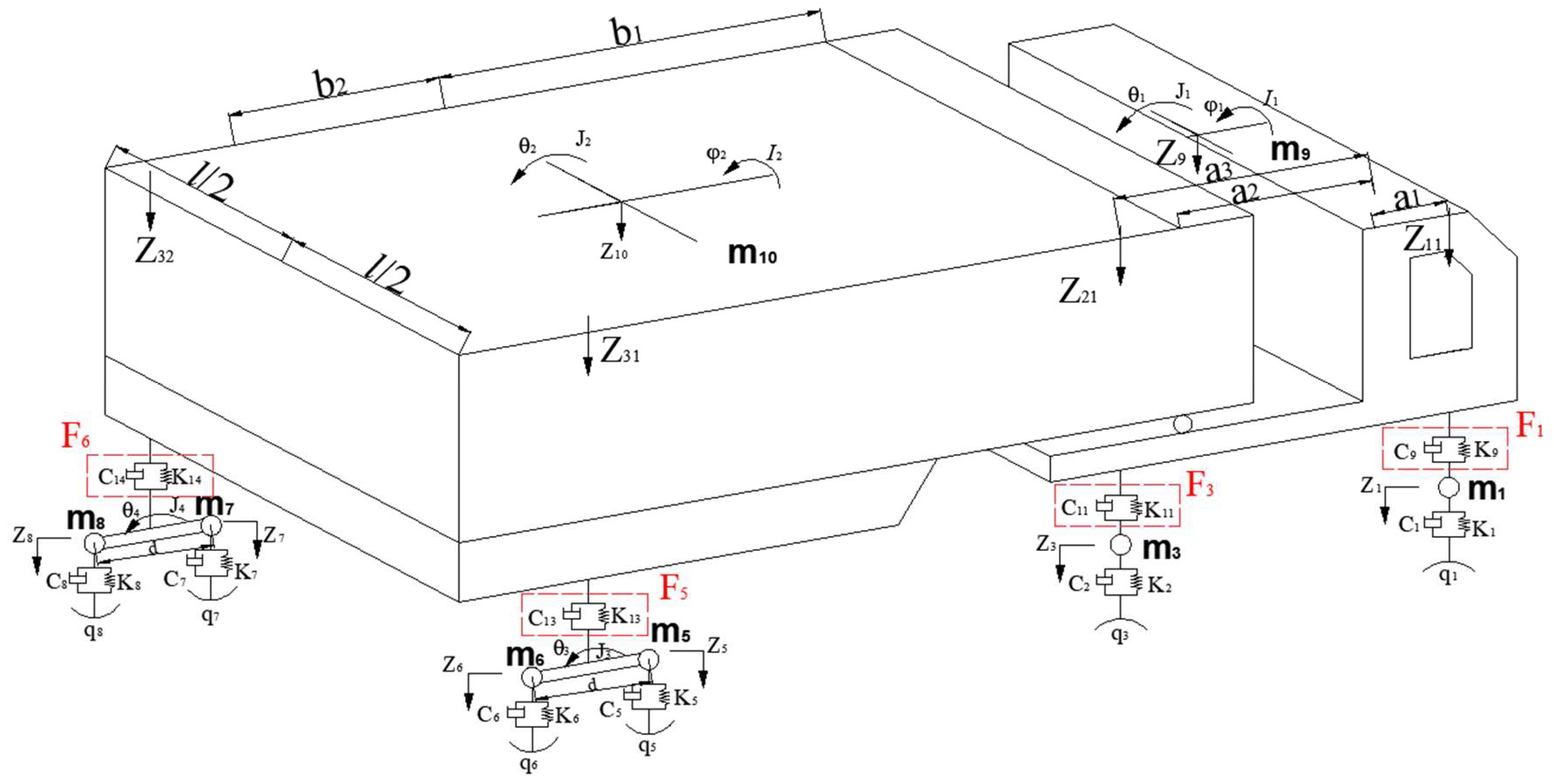
After appropriate simplification, a model of a 16-degree-of-freedom four-axle semi-trailer vehicle can be established and simplified into a centralized mass, spring, and damping model, according to Figure 3.

The degrees of freedom comprise 6 for the body vertical, trailer pitch, and trailer roll, 2 for the rear balance-suspension pitch, 4 for the vertical motion of the tractor’s front and rear axle wheel, and 4 for the trailer’s front and rear axle wheels, a total of 16 degrees of freedom.

The simplified model’s second-order vibrational differential equation can be derived using Newton’s second law as follows:

Vertical vibration of the tractor and the trailer body:

$$m_9{z}_9^{\prime \prime }+m_{10}{z}_{10}^{\prime \prime }=F_1+F_2+F_3+F_4+F_5+F_6$$

(42)

Pitching vibration of the tractor body:

$$J_1{\theta }_1^{\prime \prime }-a_2{m}_9{z}_9^{\prime \prime }=-\left(a_1+a_2\right)\left[F_1+F_2\right]+\left(a_3-a_2\right)\left[F_3+F_4\right]$$

(43)

Pitching vibration of the trailer body:

$$J_2{\theta }_2^{\prime \prime }-b_1{m}_9{z}_9^{\prime \prime }=b_2\left[F_5+F_6\right]-b_1\left[F_1+F_2+F_3+F_4\right]$$

(44)

Pitching vibration of the rear balance suspension:

$$J_3{\theta }_3^{\prime \prime }=-{\displaystyle \frac{1}{2}}d\left[c_5\left(q_5^{\prime }-z_5^{\prime }\right)+k_5\left(q_5-z_5\right)\right]+{\displaystyle \frac{1}{2}}d\left[k_6\left(q_6-z_6\right)+c_6\left(q_6^{\prime }-z_6^{\prime }\right)\right]$$

(45)

$$J_4{\theta }_4^{\prime \prime }=-{\displaystyle \frac{1}{2}}d\left[c_7\left(q_7^{\prime }-z_7^{\prime }\right)+k_7\left(q_7-z_7\right)\right]+{\displaystyle \frac{1}{2}}d\left[k_8\left(q_8-z_8\right)+c_8\left(q_8^{\prime }-z_8^{\prime }\right)\right]$$

(46)

Lateral tilt vibration of the tractor body:

$$I_1{\phi }_1^{\prime \prime }=-{\displaystyle \frac{1}{2}}l\left[F_2+F_4-F_1-F_3\right]$$

(47)

Lateral tilt vibration of the trailer body:

$$I_2{\phi }_2^{\prime \prime }=-{\displaystyle \frac{1}{2}}l\left[F_6-F_5\right]$$

(48)

Vertical vibration of the tractor’s front axle wheels:

$$m_1{z}_1^{\prime \prime }=k_1\left(q_1-z_1\right)+c_1\left(q_1^{\prime }-z_1^{\prime }\right)-F_1$$

(49)

$$m_2{z}_2^{\prime \prime }=k_2\left(q_2-z_2\right)+c_2\left(q_2^{\prime }-z_2^{\prime }\right)-F_2$$

(50)

Vertical vibration of the tractor’s rear axle wheels:

$$m_3{z}_3^{\prime \prime }=k_3\left(q_3-z_3\right)+c_3\left(q_3^{\prime }-z_3^{\prime }\right)-F_3$$

(51)

$$m_4{z}_4^{\prime \prime }=k_4\left(q_4-z_4\right)+c_4\left(q_4^{\prime }-z_4^{\prime }\right)-F_4$$

(52)

Vertical vibration of the trailer’s left and right wheels:

$$m_5{z}_5^{\prime \prime }=k_5\left(q_5-z_5\right)+c_5\left(q_5^{\prime }-z_5^{\prime }\right)-{\displaystyle \frac{1}{2}}{F}_5$$

(53)

$$m_6{z}_6^{\prime \prime }=k_6\left(q_6-z_6\right)+c_6\left(q_6^{\prime }-z_6^{\prime }\right)-{\displaystyle \frac{1}{2}}{F}_5$$

(54)

$$m_7{z}_7^{\prime \prime }=k_7\left(q_7-z_7\right)+c_7\left(q_7^{\prime }-z_7^{\prime }\right)-{\displaystyle \frac{1}{2}}{F}_6$$

(55)

$$m_8{z}_8^{\prime \prime }=k_8\left(q_8-z_8\right)+c_8\left(q_8^{\prime }-z_8^{\prime }\right)-{\displaystyle \frac{1}{2}}{F}_6$$

(56)

F₁; F₂; F₃; F₄; F₅; F₆ are the forces of each suspension system, and their expressions are

$$F_1=k_9\left(z_1-z_{11}\right)+c_9\left(z_1^{\prime }-z_{11}^{\prime }\right)$$

(57)

$$F_2=k_{10}\left(z_2-z_{12}\right)+c_{10}\left(z_2^{\prime }-z_{12}^{\prime }\right)$$

(58)

$$F_3=k_{11}\left(z_3-z_{21}\right)+c_{11}\left(z_3^{\prime }-z_{21}^{\prime }\right)$$

(59)

$$F_4=k_{12}\left(z_4-z_{22}\right)+c_{12}\left(z_4^{\prime }-z_{22}^{\prime }\right)$$

(60)

$$F_5=k_{13}\left[{\displaystyle \frac{1}{2}}\left(z_5+z_6\right)-z_{31}\right]+c_{13}\left[{\displaystyle \frac{1}{2}}\left(z_5^{\prime }+z_6^{\prime }\right)-z_{31}^{\prime }\right]$$

(61)

$$F_6=k_{14}\left[{\displaystyle \frac{1}{2}}\left(z_7+z_8\right)-z_{32}\right]+c_{14}\left[{\displaystyle \frac{1}{2}}\left(z_7^{\prime }+z_8^{\prime }\right)-z_{32}^{\prime }\right]$$

(62)

Because the pitching angle θ and the lateral tilt angle φ values in the model are generally small, there are sinθ ≈ θ, sinφ ≈ φ, so the following relationship holds:

$$z_{11}=z_9-a_1\mathit{sin}{\theta }_1-{\displaystyle \frac{1}{2}}l\mathit{sin}{\phi }_1=z_9-a_1{\theta }_1-{\displaystyle \frac{1}{2}}l{\phi }_1$$

(63)

$$z_{12}=z_9-a_1\mathit{sin}{\theta }_1+{\displaystyle \frac{1}{2}}l\mathit{sin}{\phi }_1=z_9-a_1{\theta }_1+{\displaystyle \frac{1}{2}}l{\phi }_1$$

(64)

$$z_{21}=z_9+a_3\mathit{sin}{\theta }_1-{\displaystyle \frac{1}{2}}l\mathit{sin}{\phi }_1=z_9+a_3{\theta }_1-{\displaystyle \frac{1}{2}}l{\phi }_1$$

(65)

$$z_{21}=z_9+a_3\mathit{sin}{\theta }_1+{\displaystyle \frac{1}{2}}l\mathit{sin}{\phi }_1=z_9+a_3{\theta }_1+{\displaystyle \frac{1}{2}}l{\phi }_1$$

(66)

$$z_{31}=z_{10}+b_2\mathit{sin}{\theta }_2-{\displaystyle \frac{1}{2}}l\mathit{sin}{\phi }_2=z_{10}+b_2{\theta }_2-{\displaystyle \frac{1}{2}}l{\phi }_2$$

(67)

$$z_{32}=z_{10}+b_2\mathit{sin}{\theta }_2+{\displaystyle \frac{1}{2}}l\mathit{sin}{\phi }_2=z_{10}+b_2{\theta }_2+{\displaystyle \frac{1}{2}}l{\phi }_2$$

(68)

The dynamic load of each tire can be expressed as follows using the vibration theory:

Loads of the left and right wheels for the tractor’s front axle:

$$\left\{\begin{array}{c}{F}_1\left(t\right)=k_1\left(q_1-z_1\right)+c_1\left(q_1^{\prime }-z_1^{\prime }\right)\\ F_2\left(t\right)=k_2\left(q_2-z_2\right)+c_2\left(q_2^{\prime }-z_2^{\prime }\right)\end{array}\right.$$

(69)

Rear axle as

$$\left\{\begin{array}{c}{F}_3\left(t\right)=k_3\left(q_3-z_3\right)+c_3\left(q_3^{\prime }-z_3^{\prime }\right)\\ F_4\left(t\right)=k_4\left(q_4-z_4\right)+c_4\left(q_4^{\prime }-z_4^{\prime }\right)\end{array}\right.$$

(70)

Front axle as

$$\left\{\begin{array}{c}{F}_5\left(t\right)=k_5\left(q_5-z_5\right)+c_5\left(q_5^{\prime }-z_5^{\prime }\right)\\ F_6\left(t\right)=k_6\left(q_6-z_6\right)+c_6\left(q_6^{\prime }-z_6^{\prime }\right)\end{array}\right.$$

(71)

Rear axle as

$$\left\{\begin{array}{c}{F}_7\left(t\right)=k_7\left(q_7-z_7\right)+c_7\left(q_7^{\prime }-z_7^{\prime }\right)\\ F_8\left(t\right)=k_8\left(q_8-z_8\right)+c_8\left(q_8^{\prime }-z_8^{\prime }\right)\end{array}\right.$$

(72)

The pavement roughness excitation function can be described as

$$q_1^{\prime }\left(t\right)=-2\pi n_{00}u\cdot q\left(t\right)+2\pi n_0\sqrt{G_q\left(n_0\right)u}\cdot \omega \left(t\right)$$

(73)

The pavement roughness excitation functions of the remaining wheels can be obtained from the time-domain pavement excitation simulation model of filtered white noise.

3.3. Vehicle Model of Cornering

In the cornering condition, lateral tilt of the vehicle body occurs, compared with when driving in a straight line; the corresponding lateral tilt angle φ_i and the vertical displacement difference Δh_i are produced during the period of cornering. In this study, a lateral force is applied to the vehicle body for simplification to modify the cornering condition. Taking the two-axle whole-vehicle model as an example, the wheelbase between the left and right wheels is assumed to be equal, at one; that is, c = d = e = f = l. The dynamic system of the vehicle is represented by the model, as seen in Figure 4.

The centrifugal force F required when an object with a known mass m moves with velocity v along a curve with a radius of curvature R is

$$\mathrm{F}=\mathrm{m}{\displaystyle \frac{v^2}{R}}$$

(74)

The radius of curvature R is the corresponding cornering radius of the vehicle model; the relationship between the cornering radius and the front wheel turning angle can be approximated as

$$R=L/\mathit{sin}\left(r\right)$$

(75)

Thereinto, L is the wheelbase of the vehicle; r is the front wheel turning angle of the vehicle.

In this study, it is assumed that F equals the total lateral force generated by each tire due to cornering, and the lateral force F_i of each tire is equal. Namely,

$$F=F_1+F_2+...+F_n=n\cdot F_i$$

(76)

Thereinto, I = 1, 2, 3, ..., and n represents the overall count of tires of the vehicle.

In the vehicle model, the lateral force Fi of the tire is equal to the product of the suspension stiffness ki of corresponding suspension and lateral tilt angle φ_i caused by the cornering; because the suspension stiffness is known, the corresponding lateral tilt angle φ_i can be obtained, and then the vertical displacement difference Δh_i of the suspension due to the lateral tilt can be obtained from the lateral tilt angle (because the tire and suspension characteristics on either side of the same axle are usually identical, the Δhi values for wheels on a given axle are equal); namely,

$$F_i=k_i{\phi }_i$$

(77)

$${\phi }_i={\displaystyle \frac{m\cdot v^2}{n\cdot k_i}}$$

(78)

$$\Delta h_i={\phi }_i\cdot {\displaystyle \frac{l}{2}}={\displaystyle \frac{l\cdot m\cdot v^2}{2n\cdot k_i}}$$

(79)

The results show that the change in the vehicle model is only in the suspension force equation of each suspension. The simplified physical model’s second-order vibrational differential equation can be derived using Newton’s second law as follows:

The suspension forces of the right front suspension are

$$F_{RF}=k_1\left(z_3-z_{11}+\Delta h_1\right)+c_1\left(z_3^{\prime }-z_{11}^{\prime }+\Delta h_1^{\prime }\right)$$

(80)

The suspension forces of the left front suspension are

$$F_{LF}=k_2\left(z_2-z_{12}-\Delta h_1\right)+c_2\left(z_2^{\prime }-z_{12}^{\prime }-\Delta h_1^{\prime }\right)$$

(81)

The suspension force of the rest of the suspension can be extrapolated, such that the suspension force expression of the three-axle whole-vehicle model under the cornering condition can be obtained:

$$F_A=k_{sA}\left(z_A-z_{1A}+\Delta h_1\right)+c_{sA}\left(z_A^{\prime }-z_{1A}^{\prime }+\Delta h_1^{\prime }\right)$$

(82)

$$F_A=k_{sA}\left(z_A-z_{1A}+\Delta h_1\right)+c_{sA}\left(z_A^{\prime }-z_{1A}^{\prime }+\Delta h_1^{\prime }\right)$$

(83)

$$F_C=k_{sC}\left[{\displaystyle \frac{1}{2}}\left(z_{C1}+z_{C2}\right)-z_{1C}+{\displaystyle \frac{1}{2}}\Delta h_2+{\displaystyle \frac{1}{2}}\Delta h_3\right]+c_{sC}\left[{\displaystyle \frac{1}{2}}\left(z_{C1}^{\prime }+z_{C2}^{\prime }\right)-z_{1C}^{\prime }+{\displaystyle \frac{1}{2}}\Delta h_2^{\prime }+{\displaystyle \frac{1}{2}}\Delta h_3^{\prime }\right]$$

(84)

$$F_D=k_{sD}\left[{\displaystyle \frac{1}{2}}\left(z_{D1}+z_{D2}\right)-z_{1D}-{\displaystyle \frac{1}{2}}\Delta h_2-{\displaystyle \frac{1}{2}}\Delta h_3\right]+c_{sD}\left[{\displaystyle \frac{1}{2}}\left(z_{D1}^{\prime }+z_{D2}^{\prime }\right)-z_{1D}^{\prime }-{\displaystyle \frac{1}{2}}\Delta h_2^{\prime }-{\displaystyle \frac{1}{2}}\Delta h_3^{\prime }\right]$$

(85)

Expression of the suspension force for the model of the four-axle whole vehicle in the cornering case is as follows:

$$F_1=k_9\left(z_1-z_{11}+\Delta h_1\right)+c_9\left(z_1^{\prime }-z_{11}^{\prime }+\Delta h_1^{\prime }\right)$$

(86)

$$F_2=k_{10}\left(z_2-z_{12}-\Delta h_1\right)+c_{10}\left(z_2^{\prime }-z_{12}^{\prime }-\Delta h_1^{\prime }\right)$$

(87)

$$F_3=k_{11}\left(z_3-z_{21}+\Delta h_2\right)+c_{11}\left(z_3^{\prime }-z_{21}^{\prime }+\Delta h_2^{\prime }\right)$$

(88)

$$F_4=k_{12}\left(z_4-z_{22}-\Delta h_2\right)+c_{12}\left(z_4^{\prime }-z_{22}^{\prime }-\Delta h_2^{\prime }\right)$$

(89)

$$F_5=k_{13}\left[{\displaystyle \frac{1}{2}}\left(z_5+z_6\right)-z_{31}+{\displaystyle \frac{1}{2}}\Delta h_3+{\displaystyle \frac{1}{2}}\Delta h_4\right]+c_{13}\left[{\displaystyle \frac{1}{2}}\left(z_5^{\prime }+z_6^{\prime }\right)-z_{31}^{\prime }+{\displaystyle \frac{1}{2}}\Delta h_3^{\prime }+{\displaystyle \frac{1}{2}}\Delta h_4^{\prime }\right]$$

(90)

$$F_6=k_{14}\left[{\displaystyle \frac{1}{2}}\left(z_7+z_8\right)-z_{32}-{\displaystyle \frac{1}{2}}\Delta h_3-{\displaystyle \frac{1}{2}}\Delta h_4\right]+c_{14}\left[{\displaystyle \frac{1}{2}}\left(z_7^{\prime }+z_8^{\prime }\right)-z_{32}^{\prime }-{\displaystyle \frac{1}{2}}\Delta h_3^{\prime }-{\displaystyle \frac{1}{2}}\Delta h_4^{\prime }\right]$$

(91)

3.4. Parameters of Vehicle Model

The parameters of three-axle heavy-duty vehicles [35] are shown in

Table 2. Parameters of three-axle vehicles.

Body mass, m1 (kg)	8130	Unsprung mass of intermediate shaft, mC1; mC2 (kg)	523.6
Unsprung mass of front axle, mA; mB (kg)	634.8	Unsprung mass of rear axle, mD1; mD2 (kg)	523.6
Stiffness of front axle suspension spring, KSA; KSB (N/m)	7,658,000	Damping coefficient of front suspension, CSA; CSB (Ns/m)	5073
Stiffness of rear axle suspension sping, KSC; KSD (N/m)	19,835,000	Damping coefficient of rear suspension, CSC; CSD (Ns/m)	70,396
Front tire stiffness, KtA; KtB (N/m)	1,200,000	Front tire damping coefficient, CtA; CtB (Ns/m)	4200
Intermediate tire stiffness, KtC1; KtD1 (N/m)	1,200,000	Intermediate tire damping coefficient, CtC1; CtD1 (Ns/m)	4200
Rear tire stiffness, KtC2; KtD2 (N/m)	1,200,000	Rear tire damping coefficient, CtC2; CtD2 (Ns/m)	4200
Pitching moment of inertia of body, J1(N·m2)	61,230	Moment of inertia of rear balance suspension, J2; J3(N·m2)	43.5
Lateral tilt moment of inertia of the body, I (N·m2)	47,630

, where a = 3.81 m, b = 2.36 m, d = 1.88 m, and l = 2.44 m.

The model parameters of the four-axle semi-trailer vehicle [36] are shown in

Table 3. Parameters of four-axle vehicles.

Sprung mass of the tractor, m9 (kg)	2730	Sprung mass of the trailer, m10(kg)	13,750
Unsprung mass of the tractor front wheel, m1; m2 (kg)	530	Unsprung mass of the trailer front wheel, m5; m7 (kg)	457
Unsprung mass of the tractor rear wheel, m3; m4 (kg)	530	Unsprung mass of the trailer rear wheel, m6; m8 (kg)	457
Tire stiffness of tractor front wheel, K1; K2 (N/m)	1,250,000	Tire damping coefficient of tractor front wheel, C1; C2 (Ns/m)	4320
Tire stiffness of tractor rear wheel, K3; K4 (N/m)	2,470,000	Tire damping coefficient of tractor rear wheel, C3; C4 (Ns/m)	4320
Tire stiffness of trailer front wheel, K5; K7 (N/m)	2,760,000	Tire damping coefficient of trailer front wheel, C5; C7 (Ns/m)	4320
Tire stiffness of trailer rear wheel, K6; K8 (N/m)	2,760,000	Tire damping coefficient of trailer rear wheel, C6; C8 (Ns/m)	4320
Stiffness of tractor front axle suspension spring, K9; K10 (N/m)	763,000	Damping coefficient of suspension of tractor front axle, C9; C10 (Ns/m)	3918
Stiffness of tractor rear axle suspension spring, K11; K12 (N/m)	820,000	Damping coefficient of suspension of tractor rear axle, C11; C12 (Ns/m)	11,700
Stiffness of rear balance suspension axle, K13; K14 (N/m)	1,880,000	Damping coefficient of suspension of rear balance suspension axle, C13; C14 (Ns/m)	23,600
Pitching moment of inertia of tractor, J1(N·m2)	62,500	Pitching moment of inertia of trailer, J2(N·m2)	979,300
Pitching moment of rear balance suspension, J3; J4(N·m2)	27.3	Lateral tilt moment of inertia of trailer, I1(N·m2)	386,070
Lateral tilt moment of inertia of tractor, I2(N·m2)	604,900

, where a₁ = 0.831 m, a₂ = 2.232 m, a₃ = 2.746 m, b₁ = 2.529 m, b₂ = 2.826 m, d = 1.25 m, and l = 2.6 m.

3.5. Numerical Simulation of Vehicle Model

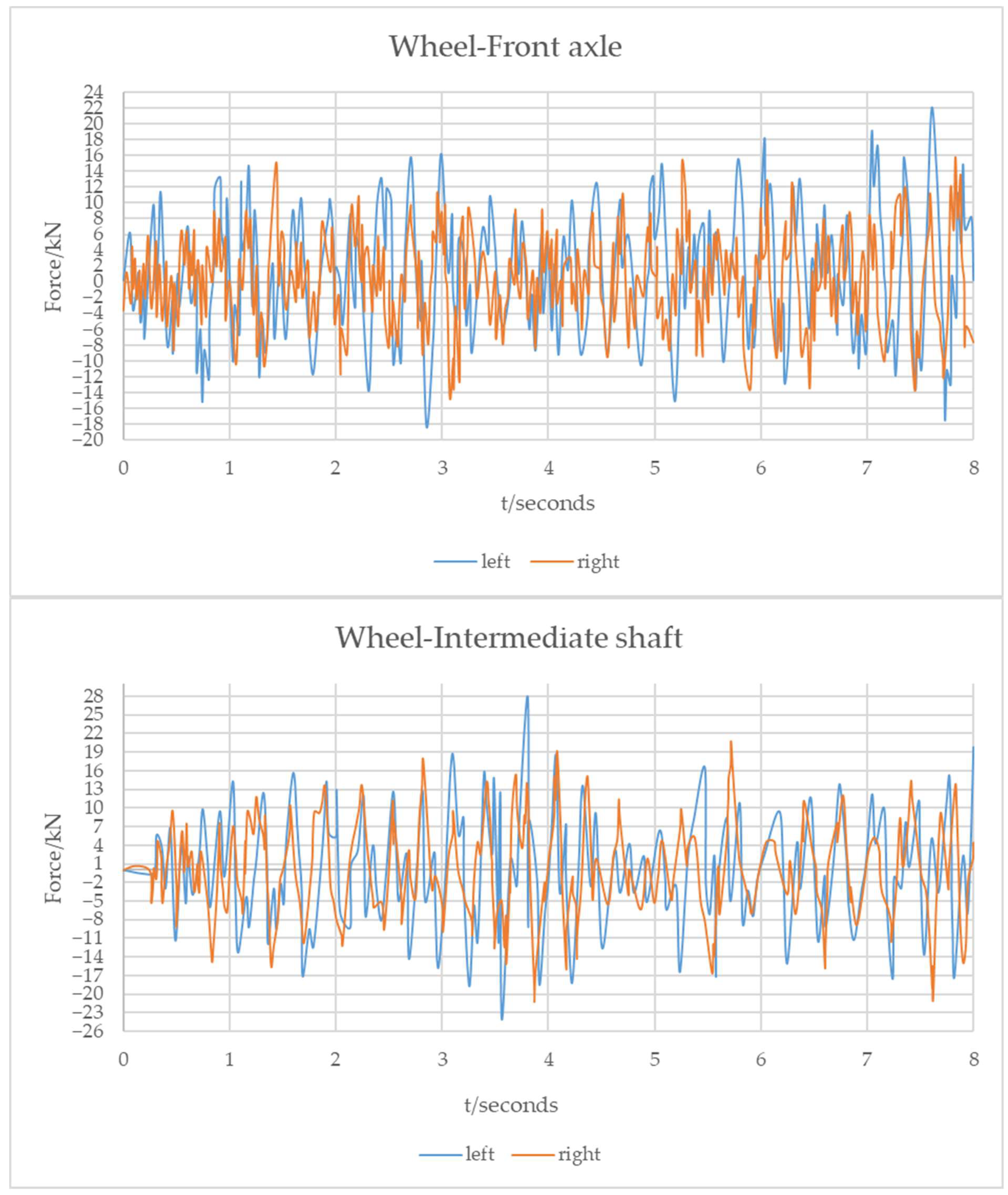
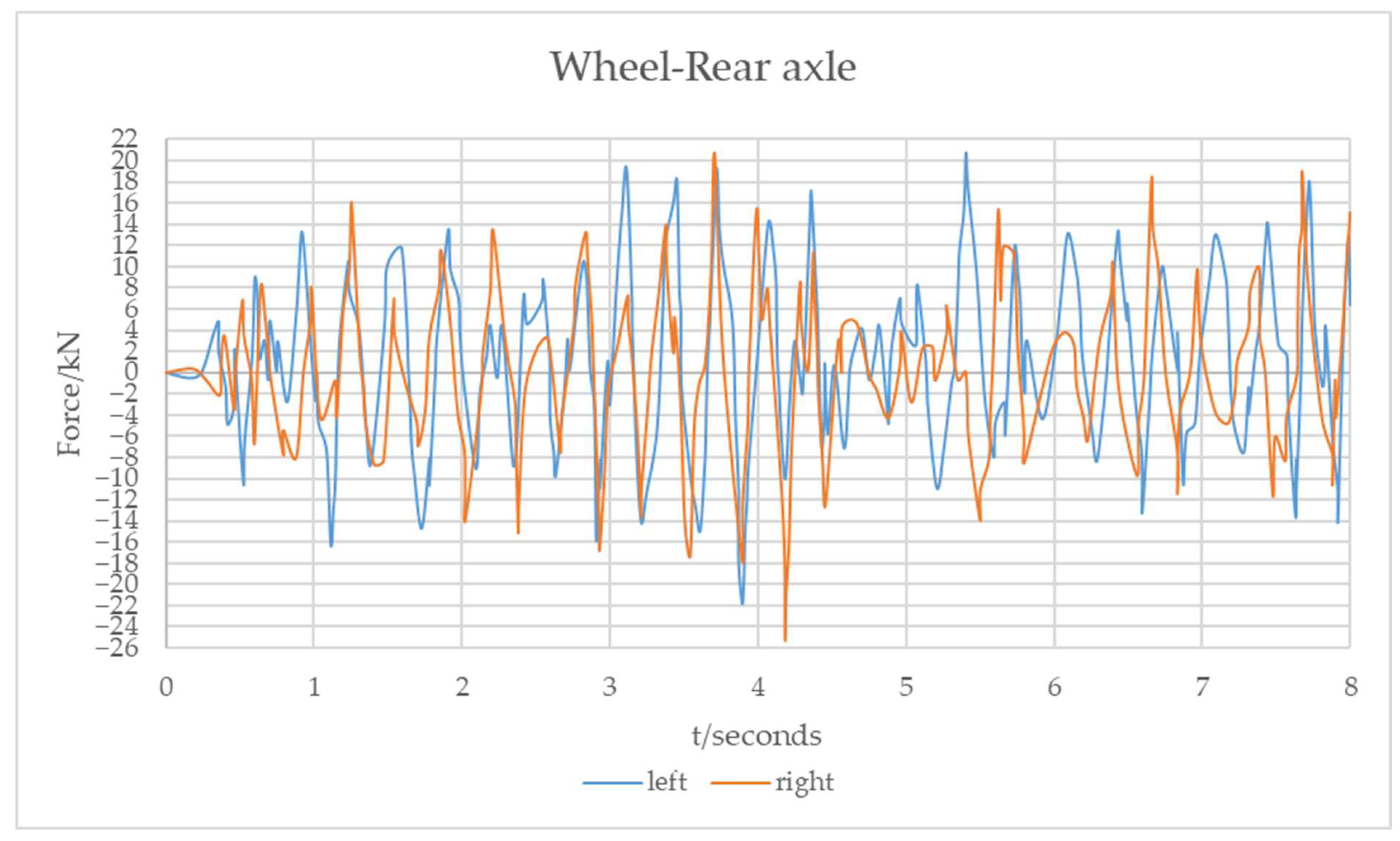
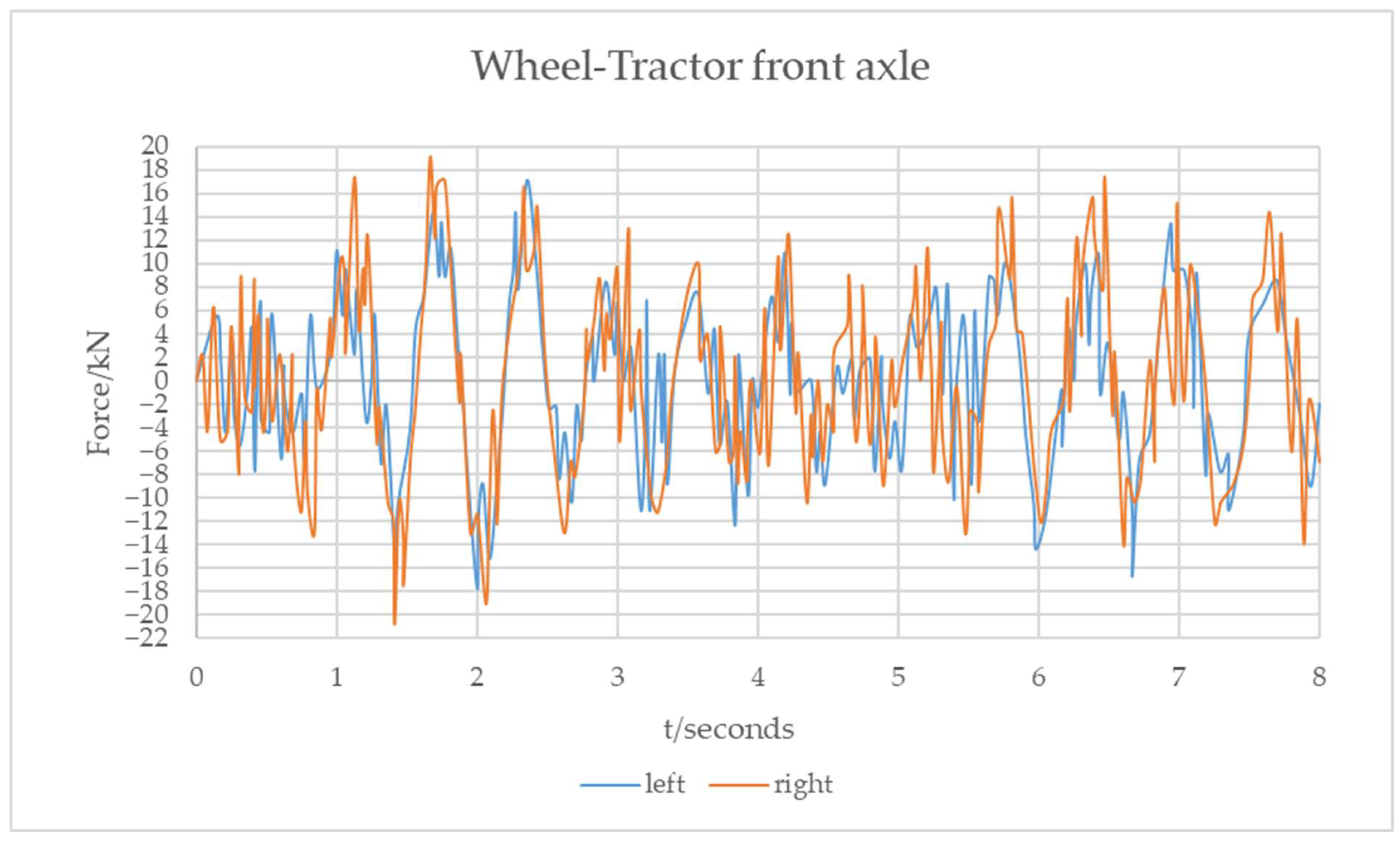
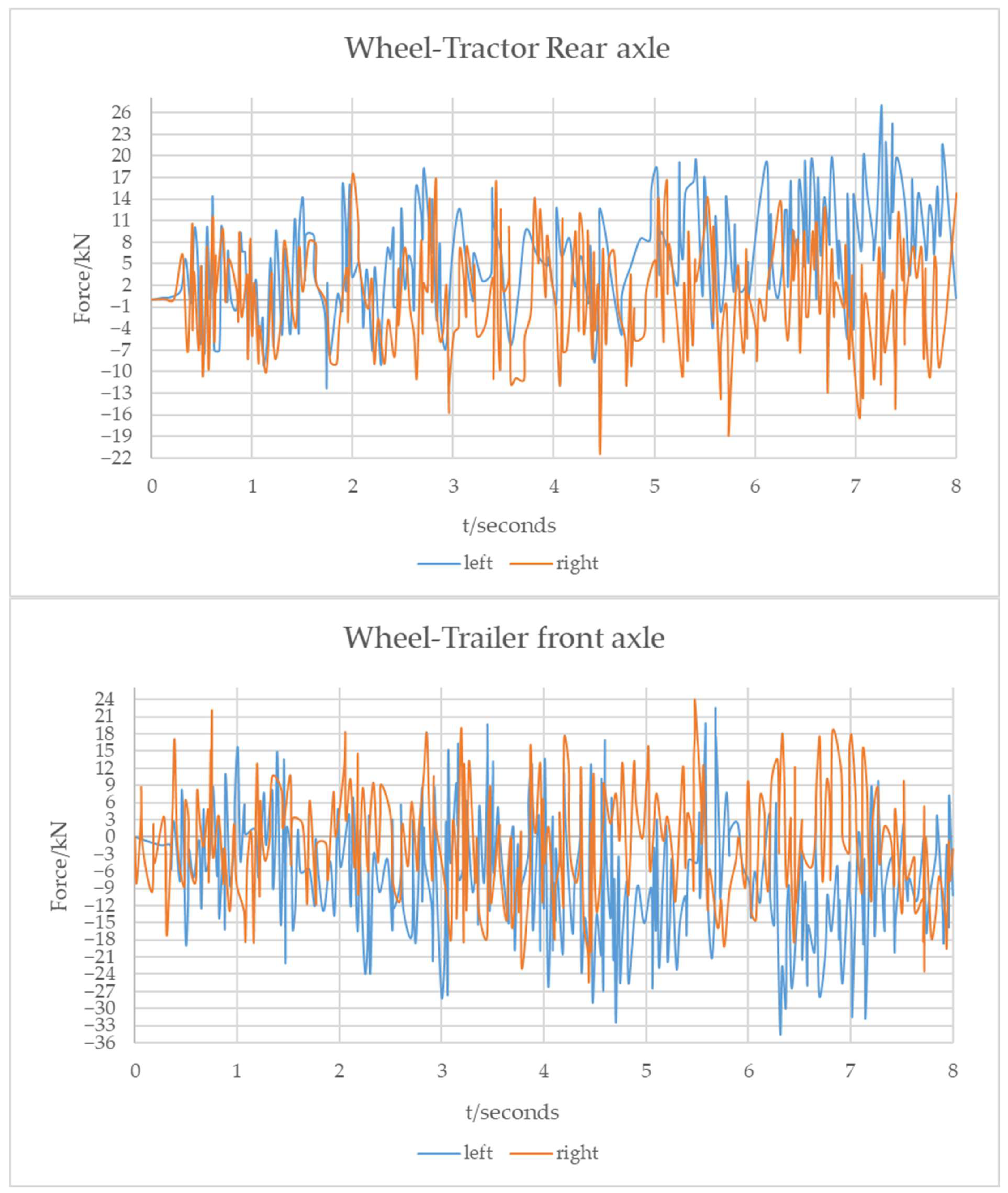
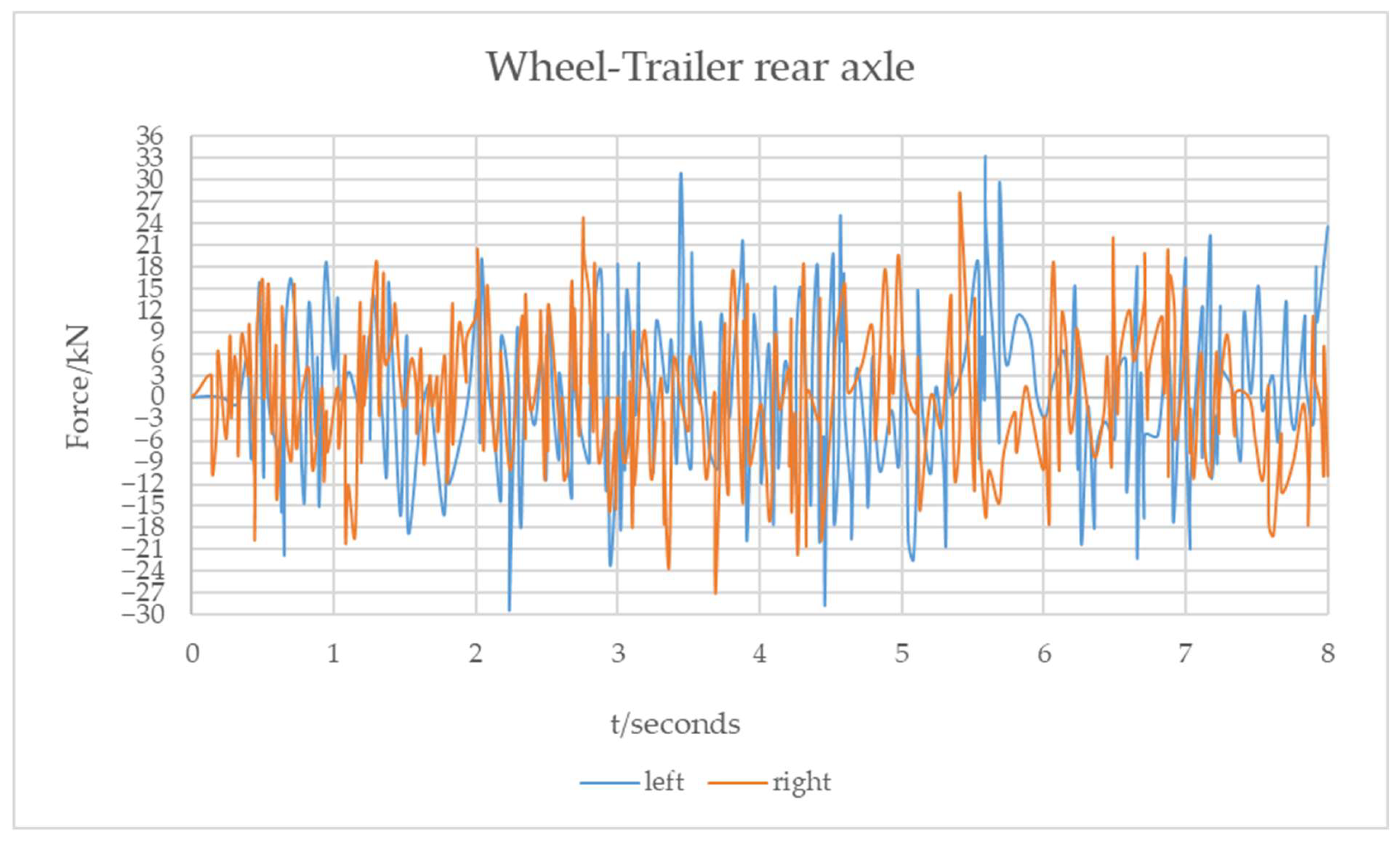
The vibration model of the three-axle and four-axle heavy-duty vehicle was simulated using Simulink software, assuming that the vehicle travels in a straight line at a uniform speed, the vehicle speed is v = 20 m/s, and the pavement roughness coefficient is considered according to the grade B pavement; that is, $G_d\left(n_0\right)=64\times 10^{-6}{\mathrm{m}}^3$. The time-domain curves of the system freedom and dynamic load were obtained under the condition of simulated pavement excitation by filtered white noise, as shown in Figure 5 and Figure 6.

The study presents the simulation of the vehicle model through Simulink software, which is different from the actual situation. The uneven pavement surface is first passed through by the tires on both sides of the front axle of the three-axle or four-axle vehicle; at this point, the contact pavement surface is left completely flat for the rest of the tires; as the vehicle continues to be moved forward, the surface excitation of filtered white noise is successively received by the intermediate shaft and the rear axle tires. The above figures compare the intermediate and rear wheels of the three-axle vehicle with the front wheels. A lag in the initial output curve response is also observed for the four-axle vehicle.

4. Simulation and Analysis of Heavy-Duty Whole Vehicles

The dynamic load of vehicle tires is a waveform curve that changes continuously with time, and when analyzing the pattern of dynamic load variation under different vehicle conditions and pavement roughness parameters, it is essential to use suitable evaluation indicators to describe it. The following two types are used in this study:

• Root-mean-square values of the dynamic load

RMS is the extraction of the square root of the average of the sum of squares of the dynamic load values within a certain time history. The RMS expression is

$$R_i=\sqrt{{\displaystyle \frac{{\sum }_{i=1}^N{F}_1^2\left(t_i\right)}{N}}}=\sqrt{{\displaystyle \frac{F_1^2\left(t_1\right)+F_1^2\left(t_2\right)+\cdot \cdot \cdot +F_1^2\left(t_N\right)}{N}}}$$

(92)

2.

Dynamic load coefficient

The RMS of the dynamic load divided by the tire’s static axle load is the dynamic load factor D.

①

Three-axle vehicle

Front axle:

$$D_1={\displaystyle \frac{R_1}{\left(m_A+\frac{b}{a+b}{m}_1\right)g}}$$

(93)

$$D_2={\displaystyle \frac{R_2}{\left(m_B+\frac{b}{a+b}{m}_1\right)g}}$$

(94)

Intermediate shaft:

$$D_3={\displaystyle \frac{R_3}{\left(m_{C_1}+\frac{a}{2\left(a+b\right)}{m}_1\right)g}}$$

(95)

$$D_5={\displaystyle \frac{R_5}{\left[m_{C_2}+\frac{b}{2\left(a+b\right)}{m}_1\right]g}}$$

(96)

Rear axle:

$$D_4={\displaystyle \frac{R_4}{\left(m_{D_1}+\frac{a}{2\left(a+b\right)}{m}_1\right)g}}$$

(97)

$$D_6={\displaystyle \frac{R_6}{\left[m_{D_2}+\frac{b}{2\left(a+b\right)}{m}_1\right]g}}$$

(98)

②

Four-axle vehicle

Tractor front axle:

$$D_1={\displaystyle \frac{R_1}{\left(m_1+\frac{a_3}{a_1+a_3}{m}_9+\frac{b_1}{b_1+b_3}\frac{a_3-a_2}{a_1+a_3}{m}_{10}\right)g}}$$

(99)

$$D_2={\displaystyle \frac{R_2}{\left(m_2+\frac{a_3}{a_1+a_3}{m}_9+\frac{b_1}{b_1+b_3}\frac{a_3-a_2}{a_1+a_3}{m}_{10}\right)g}}$$

(100)

Tractor rear axle:

$$D_3={\displaystyle \frac{R_3}{\left(m_3+\frac{a_1}{a_1+a_3}{m}_9+\frac{b_1}{b_1+b_2}\frac{a_1+a_2}{a_1+a_3}{m}_{10}\right)g}}$$

(101)

$$D_4={\displaystyle \frac{R_4}{\left(m_4+\frac{a_1}{a_1+a_3}{m}_9+\frac{b_1}{b_1+b_2}\frac{a_1+a_2}{a_1+a_3}{m}_{10}\right)g}}$$

(102)

Trailer front axle:

$$D_5={\displaystyle \frac{R_5}{\left(m_5+\frac{1}{2}\frac{b_2}{b_1+b_2}{m}_{10}\right)g}}$$

(103)

$$D_7={\displaystyle \frac{R_7}{\left(m_7+\frac{1}{2}\frac{b_2}{b_1+b_2}{m}_{10}\right)g}}$$

(104)

Trailer rear axle:

$$D_6={\displaystyle \frac{R_6}{\left(m_6+\frac{1}{2}\frac{b_1}{b_1+b_2}{m}_{10}\right)g}}$$

(105)

$$D_8={\displaystyle \frac{R_8}{\left(m_8+\frac{1}{2}\frac{b_1}{b_1+b_2}{m}_{10}\right)g}}$$

(106)

These two evaluation indices were employed to assess the effects of varying pavement roughness coefficients, different loads, different vehicle speeds, and different cornering radii on dynamic loads. Thereinto,

• Table 1’s four grades—A, B, C, and D—are chosen to represent four different pavement roughness coefficients;
• The load is selected from four situations: no-load, standard load, full load, and 0.2-times overload;
• The vehicle speeds are 6 m/s, 14 m/s, and 25 m/s;
• The cornering radii are 71 m, 36 m, and 24 m, and the corresponding front wheel turning angles are 5°, 10°, and 15°, respectively.

4.1. Effect of Roughness Coefficient on Dynamic Load

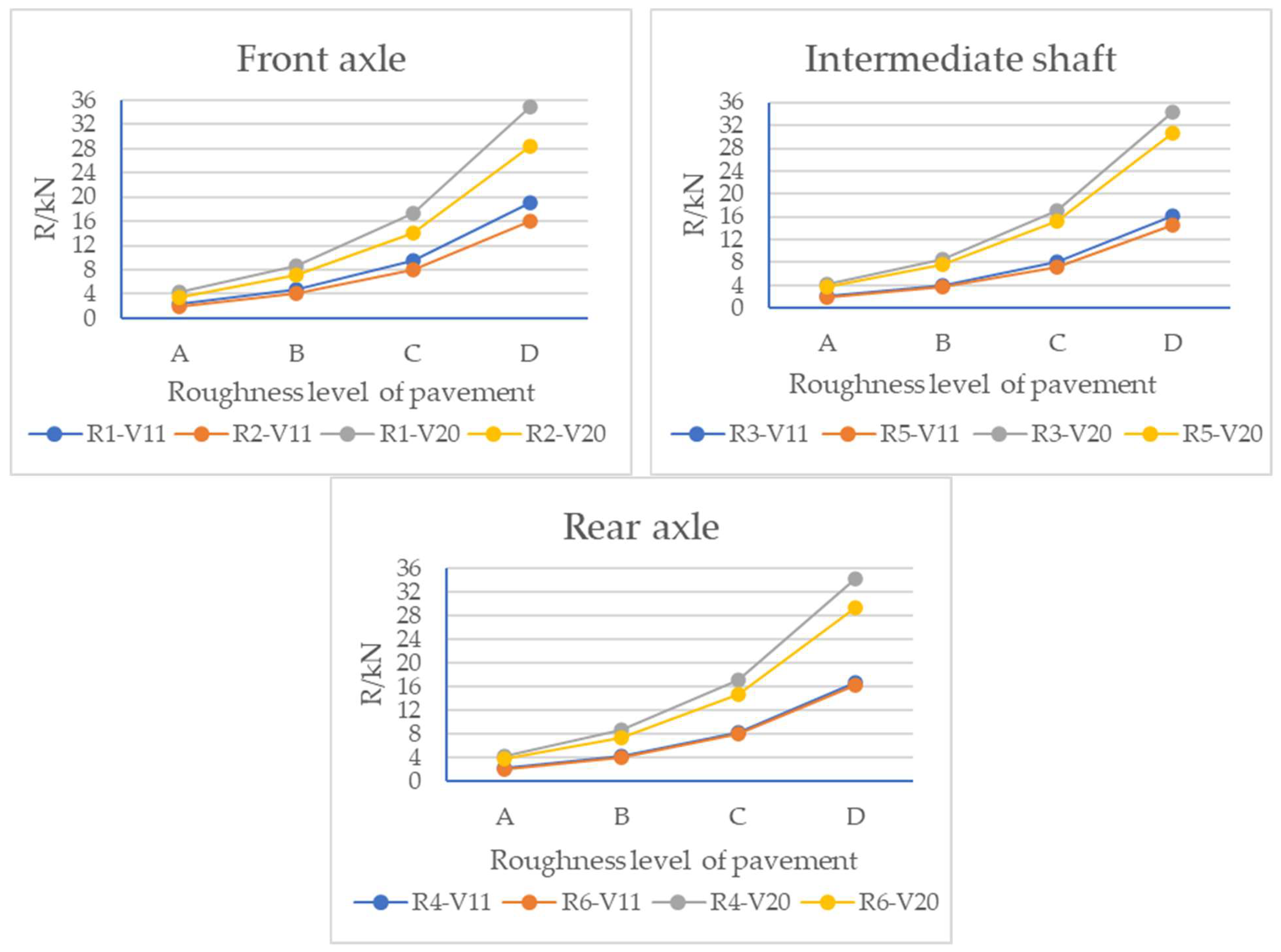
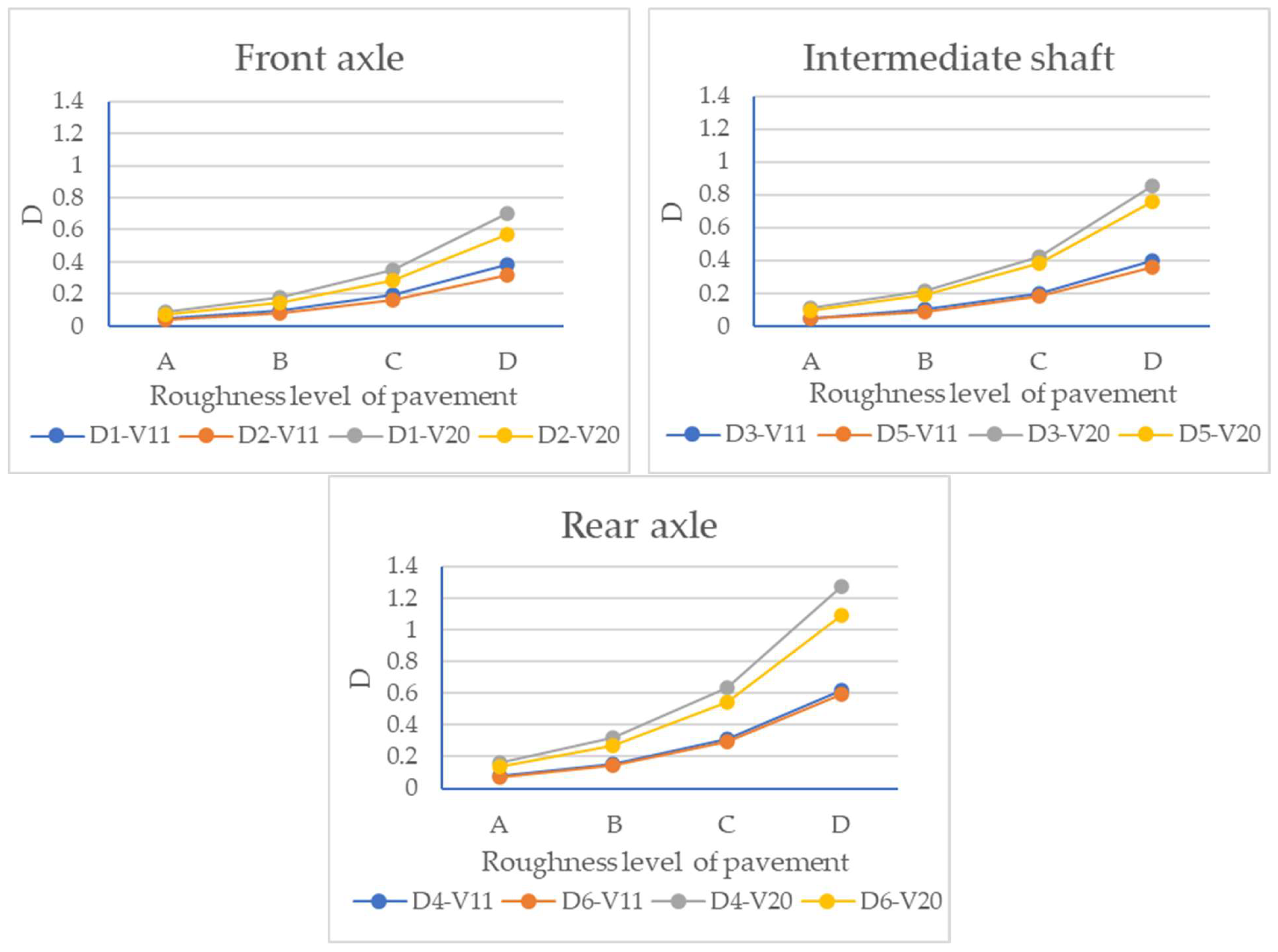
The vehicle is the standard load, and the simulation was carried out at speeds of 11 m/s and 20 m/s. The root-mean-square value and dynamic load coefficient of the dynamic load of each axle wheel of the three-axle vehicle were obtained, as shown in Figure 7 and Figure 8.

The following can be observed from the figures:

• With the deterioration in the pavement roughness grade from grade A to grade D, the root-mean-square value and dynamic load coefficient of each wheel of the three-axle vehicle gradually increase rapidly with a nonlinear trend. This shows that the greater the fluctuation in the longitudinal section of the pavement surface, the more intense the vibration generated by the wheels.
• The root-mean-square value and dynamic load coefficient of the wheel forces are more significantly impacted by the pavement surface roughness as the vehicle speed increases.
• Under the same pavement surface roughness level and the same speed, the average dynamic load index of the rear axle wheel is larger than that of the front axle and the intermediate shaft.

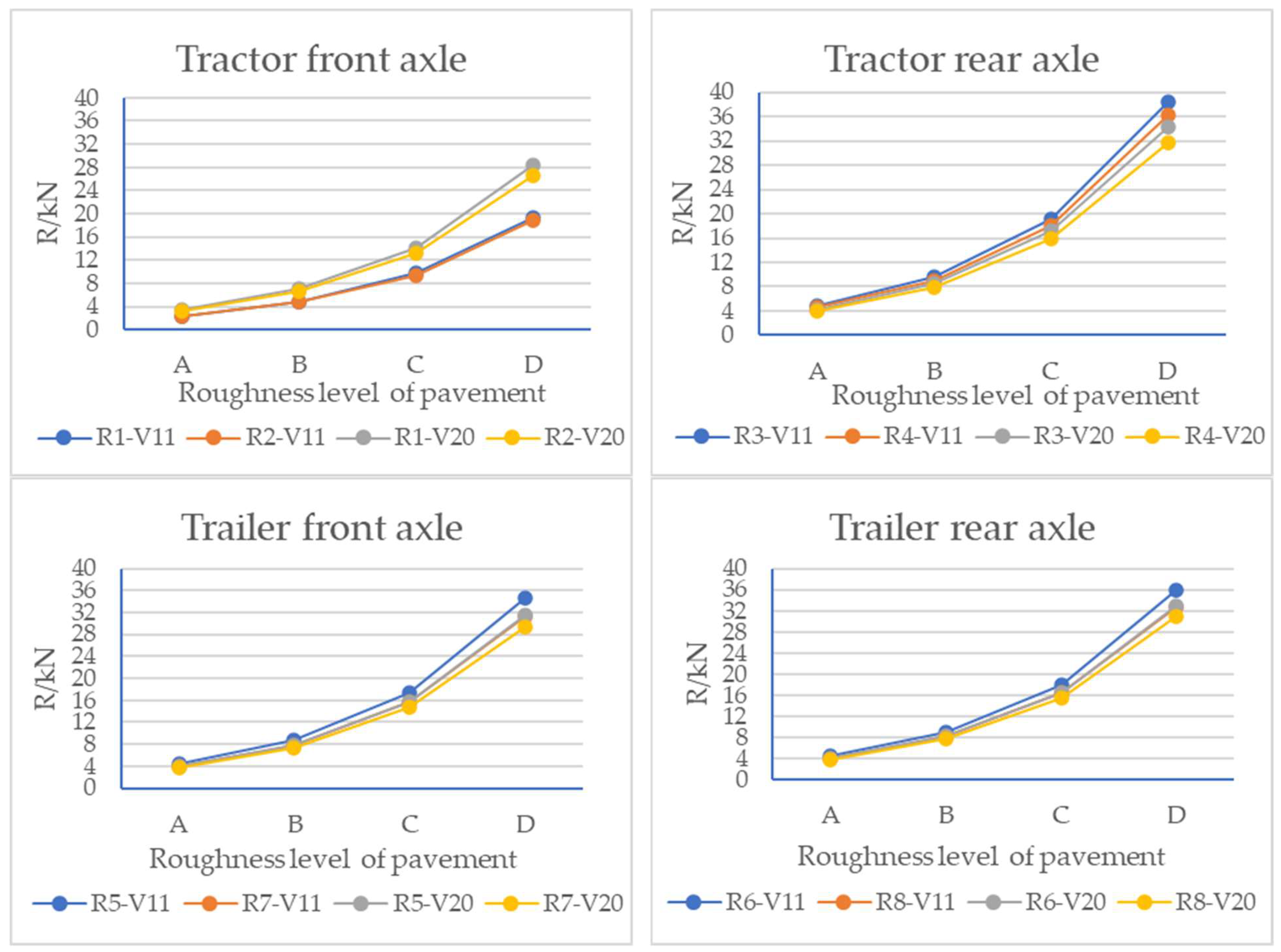
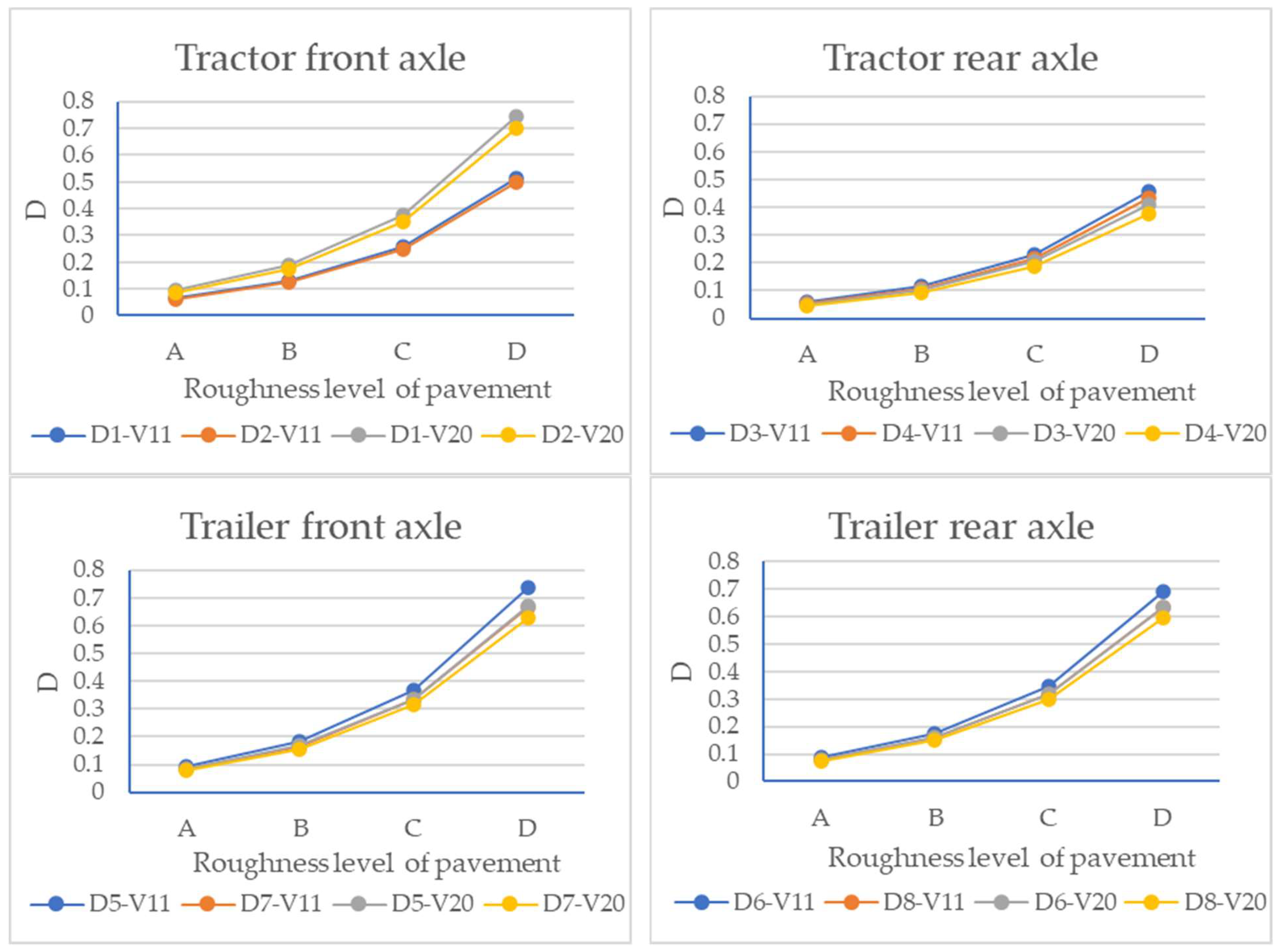
The root-mean-square value of the dynamic load and vibratory loading coefficient of each axle wheel of the four-axle vehicle are shown in Figure 9 and Figure 10.

The figures show the following:

• The variation law of the root-mean-square value and dynamic load coefficient of the dynamic load of the four-axle vehicle is similar to that of the three-axle vehicle, and with a deterioration in roughness, the root-mean-square value of the dynamic load and the dynamic load coefficient of each wheel increase nonlinearly. The higher the vehicle speed, the greater the influence of the pavement surface roughness on the root-mean-square value and dynamic load coefficient of the dynamic load.
• The variation in the dynamic load coefficient of the trailer is greater than that of the tractor, indicating that the roughness has a greater impact on the trailer of the four-axle vehicle.

4.2. Effect of Load on Dynamic Load

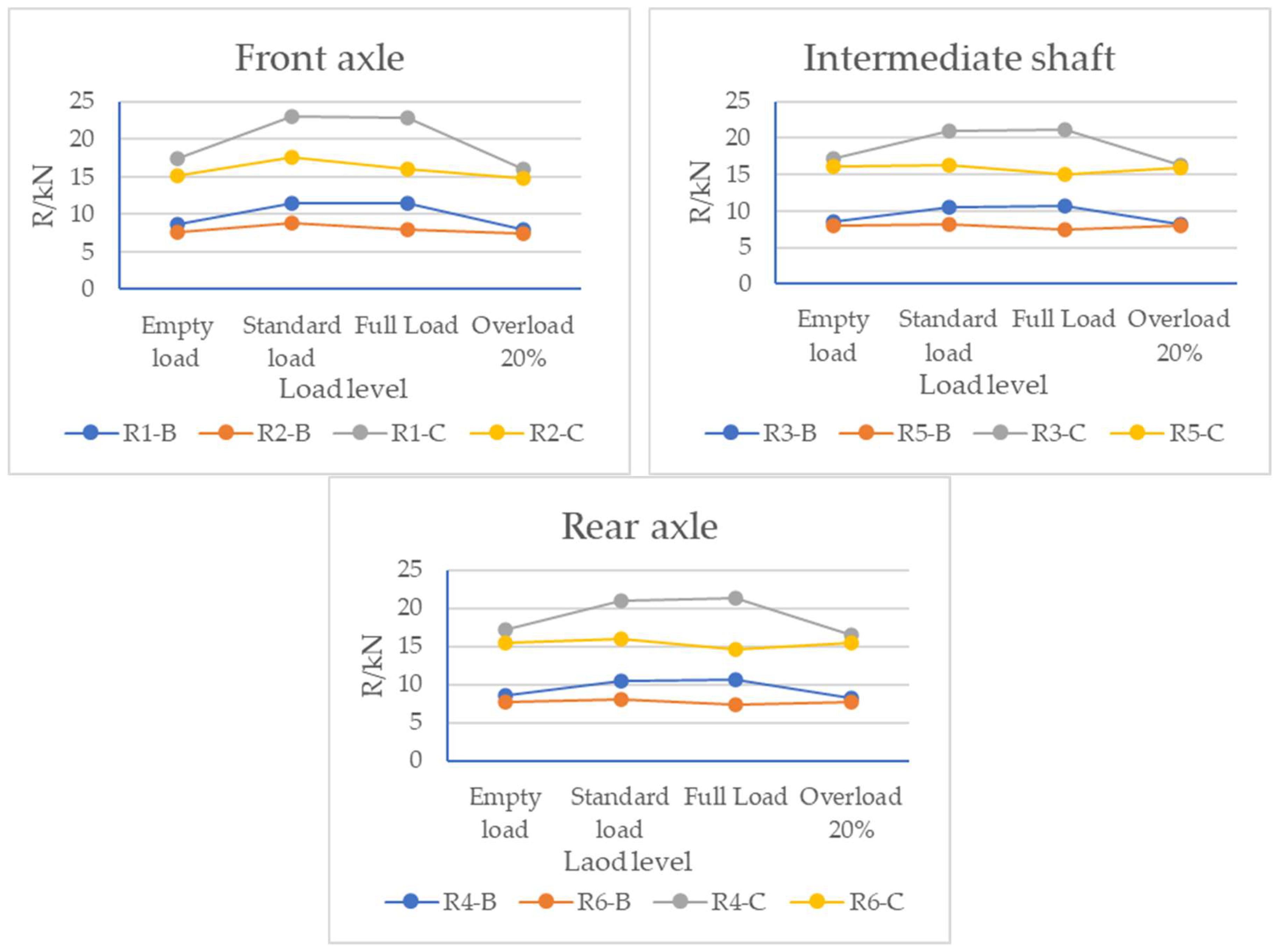
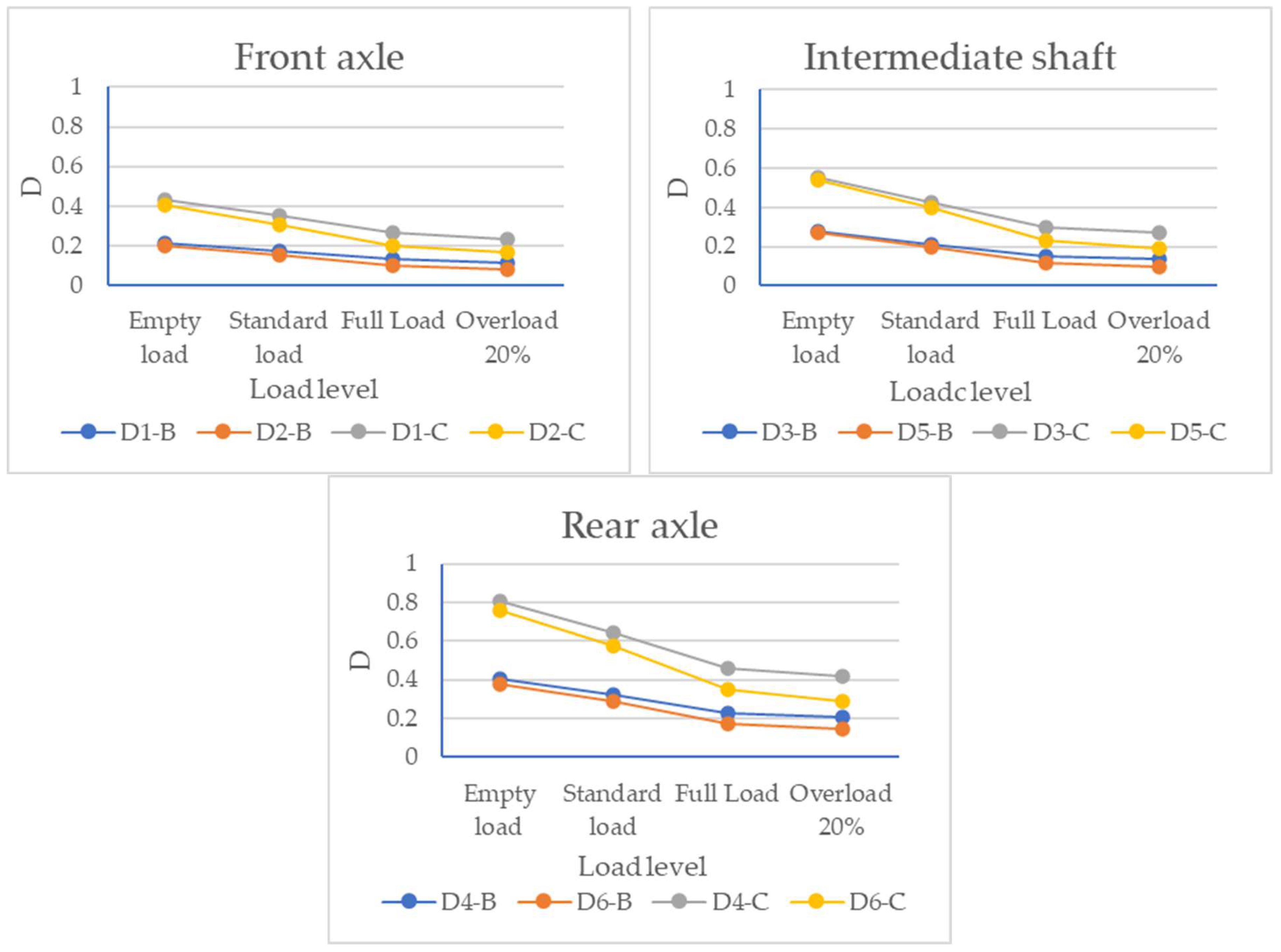
It is presumed that the load mass is evenly distributed within the vehicle. Considering that the vehicle is driving at a speed of 17 m/s on a pavement of B and C grade, the root-mean-square value of the dynamic load and the dynamic load coefficient of each axle wheel of the three-axle vehicle are as shown in Figure 11 and Figure 12.

The figures show the following:

• The root-mean-square value of the dynamic load of each wheel of the three-axle vehicle increases slowly with an increase in load, and its impact becomes greater as the roughness of the pavement surface. At the same time, the R value of each wheel decreases from full load to overload, indicating that a higher load contributes to preventing the vehicle from vibrating.
• The dynamic load coefficient of each wheel shows a downward trend with an increase in load, and this downward trend gradually slows down as the load increases. The results show that an increase in vehicle load inhibits the vibration of the vehicle, while the slowdown in the downward trend indicates that the influence of the dynamic load coefficient is greater when the vehicle is lightly loaded.
• The dynamic load coefficient of the rear axle wheel of the three-axle vehicle is greater than that of the front wheel, and the smaller the vehicle load, the greater the difference. This is mainly because the load weight of three-axle vehicles is concentrated in the rear compartment of the vehicle.

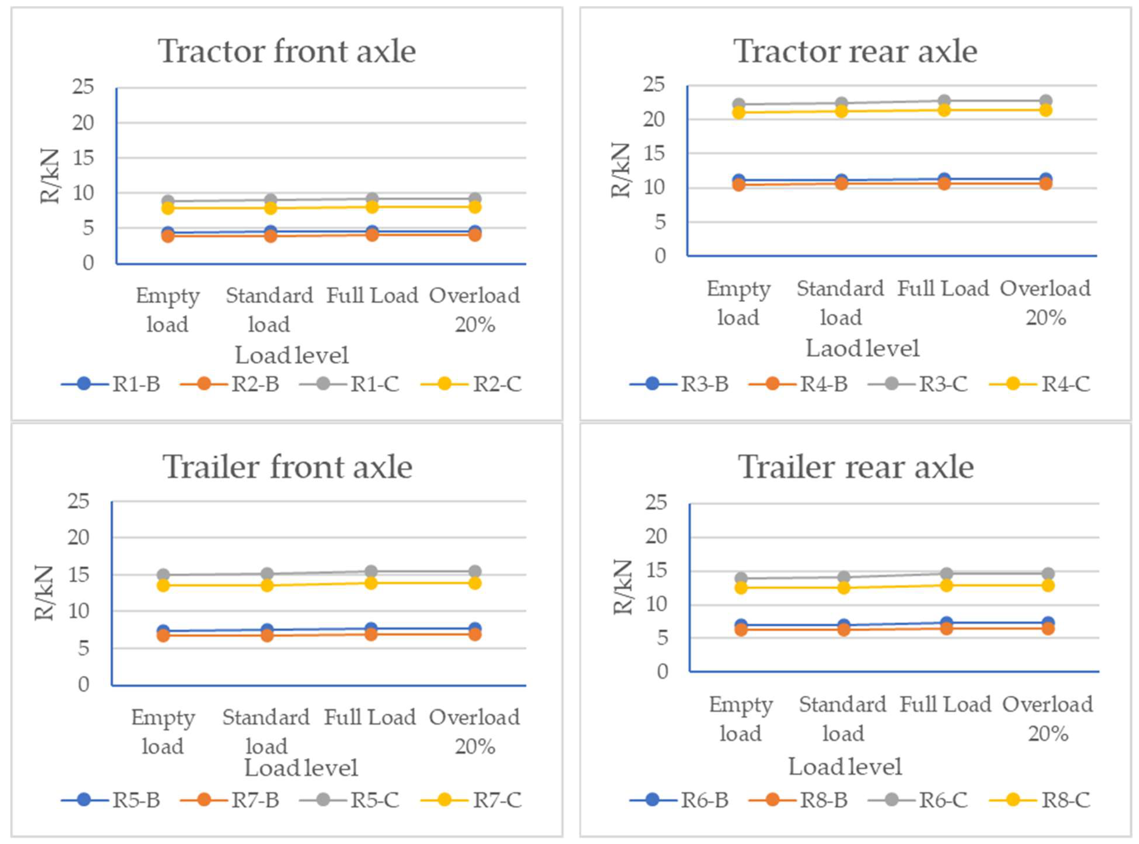
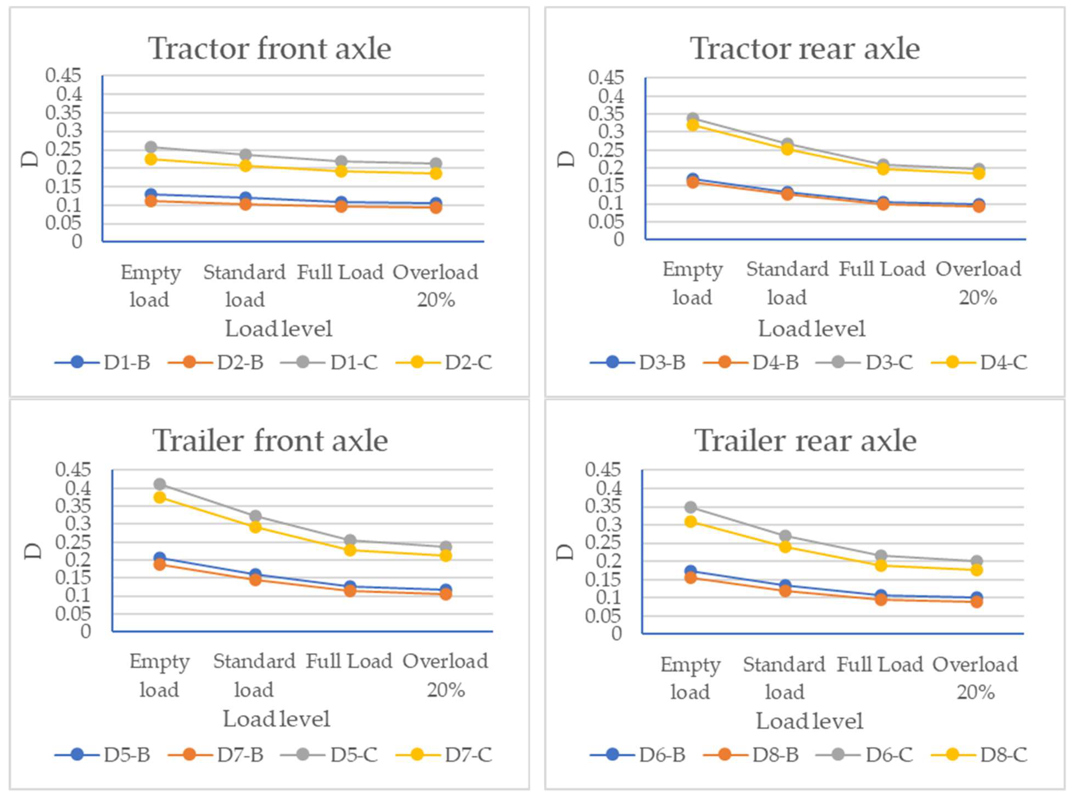
The root-mean-square value of the dynamic load and the dynamic load coefficient of each axle wheel of the four-axle vehicle are shown in Figure 13 and Figure 14.

As can be seen from the figures:

• The root-mean-square value of the dynamic load of each wheel does not change much in different load states, showing a trend of increasing slowly.
• The dynamic load coefficient for each wheel likewise decreases as the load increases. The dynamic load coefficient of the tractor wheel is larger than that of the trailer, and the smaller the vehicle load, the greater the difference between the two. This indicates that the increase in the vehicle load has a higher effect on the four-axle vehicle tractor’s dynamic load.

4.3. Effect of Vehicle Speed on Dynamic Load

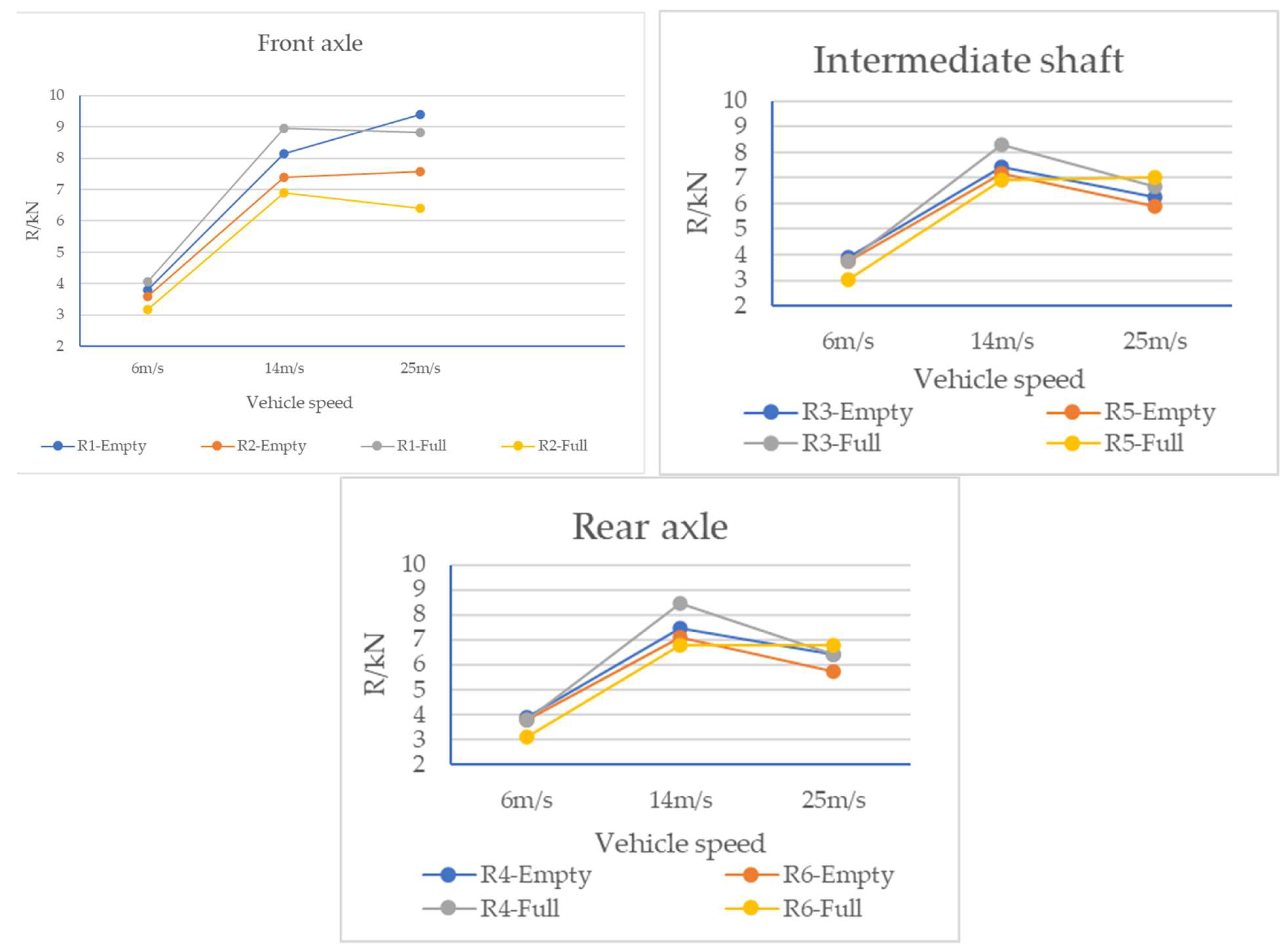
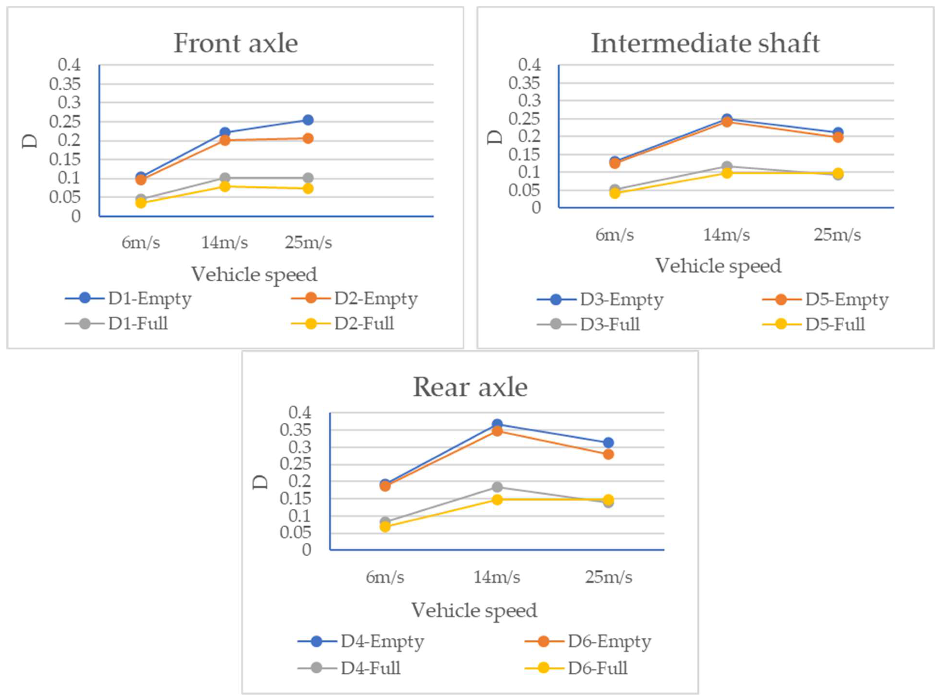
Assuming that the vehicle is driving on a B-grade pavement surface at speeds of 6 m/s, 14 m/s, and 25 m/s, respectively, at no-load and full load, the root-mean-square value of the dynamic load and the dynamic load coefficient of each axle wheel of the three-axle vehicle can be obtained through simulation, as shown in Figure 15 and Figure 16.

The figures show the following:

• As speed increases, the root-mean-square value of the dynamic load for each wheel of a three-axle vehicle increases first and then tends to flatten or decrease. The dynamic load coefficient of the front axle gradually increases, while those of the intermediate shaft and rear axle increase first and then decrease. This is mainly because, as the speed changes, the wheel vibration frequency also changes; when the wheel vibration frequency is close to or equal to pavement excitation frequency, the wheel and pavement surface resonate, resulting in an increase in the degree of wheel vibration, and the corresponding dynamic load index also increases. When the vehicle speed continues to increase, the dynamic load index exhibits a declining trend, the wheel’s vibration frequency is far from the pavement surface’s excitation frequency, and the resonance between the wheel and pavement surface vanishes.
• At different speeds, the dynamic load of the vehicle without a load is greater than that of the vehicle with a full load, which also shows that an increase in vehicle load plays a certain role in inhibiting the vibration of the wheel.

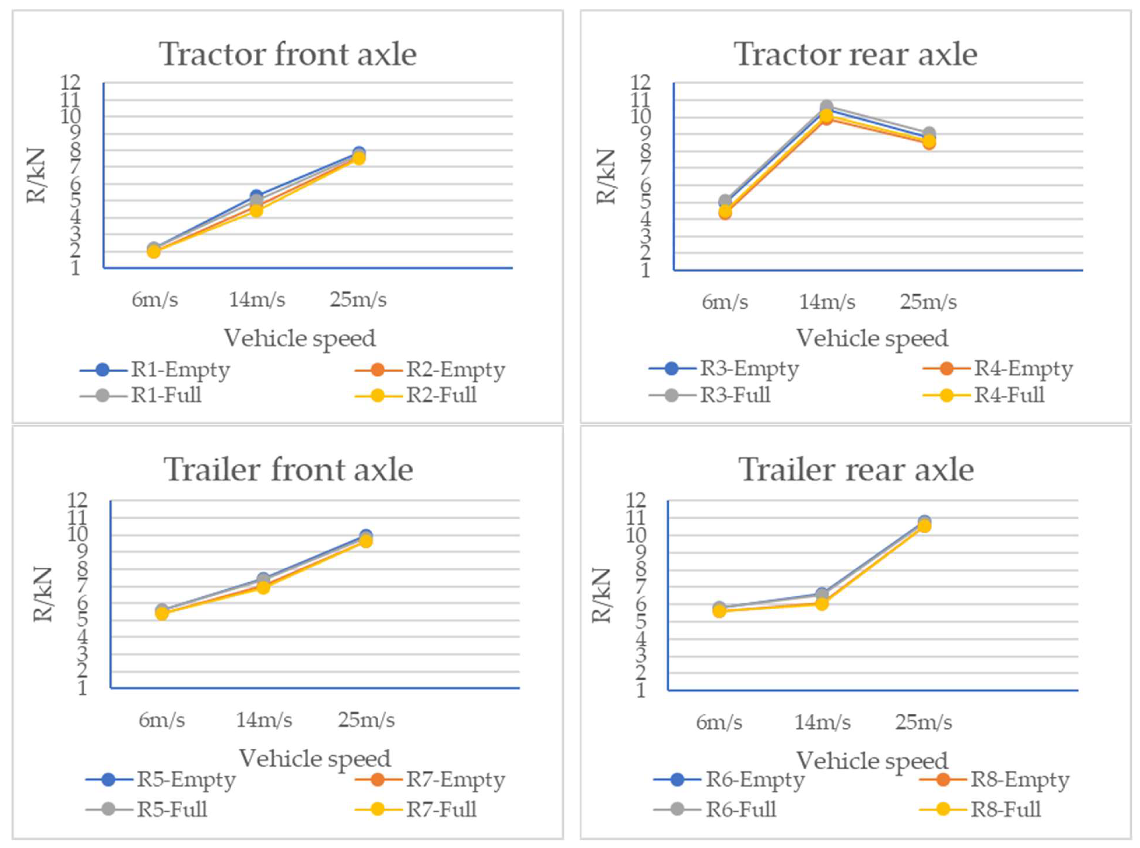
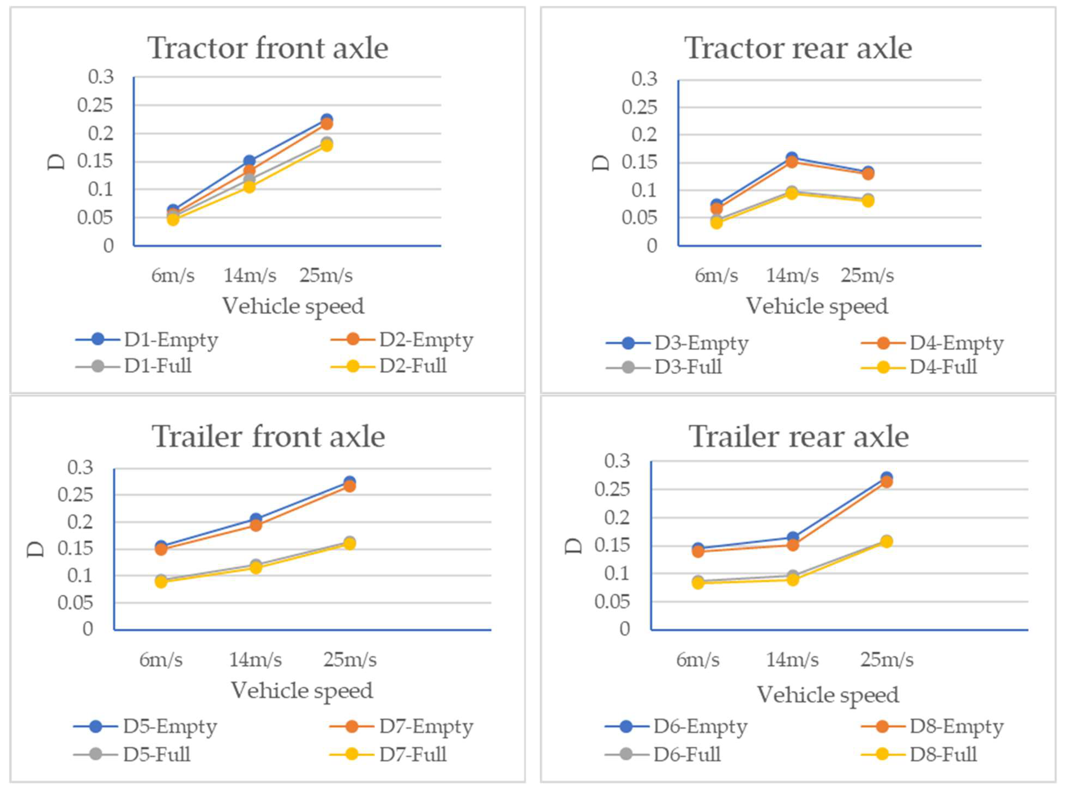
The root-mean-square value of the dynamic load and the load coefficient of each axle wheel of the four-axle vehicle are shown in Figure 17 and Figure 18.

The figure shows the following:

• With an increase in speed, the dynamic load index, the front axle of the four-axle vehicle tractor, and those of the front and rear axle wheels of the trailer all show an increasing trend, while those of the rear axle wheels of the tractor show a decreasing trend. This is also due to the interaction between the vibration frequency of the rear wheel of the tractor and the frequency of the pavement surface excitation.
• For the four-axle vehicle, whether it is at the no-load or full load has little influence on its dynamic load index.

4.4. Effect of Vehicle Lateral Tilt on Dynamic Load

Assuming that the vehicle turns right at speeds of 6 m/s and 14 m/s, respectively, on a B-grade pavement curve with 5°, 10°, and 15°angles (turning radii of 71 m, 36 m and 24 m) at no-load and full load, respectively, and the lateral tilt condition of the vehicle is simulated, the root-mean-square value of the dynamic load and the dynamic load coefficient of each axle wheel of the three-axle vehicle can be obtained, as shown in Figure 19 and Figure 20.

The figures show the following:

• The turning radius has little influence on the dynamic load index of each wheel, and the faster the vehicle’s speed, the greater its dynamic load index.
• When the vehicle is cornering, the dynamic load indices of the left and right wheels are not the same, while those of the wheels on both sides of the front axle are very close at lower speeds, and the dynamic load index of the left wheel of the front axle is greater than that of the right wheel at higher speeds. At both speeds, the dynamic load index of the left wheel of the intermediate shaft and rear axle is larger than that of the right wheel. At the same time, the dynamic load index of the left wheel increases slowly with an increase in cornering angle, and that of the right wheel decreases slowly with an increase in cornering angle. This is mainly due to the lateral tilt caused by the cornering of the vehicle, which is affected by centrifugal force, resulting in a larger dynamic load index of the left wheel than that of the right wheel.

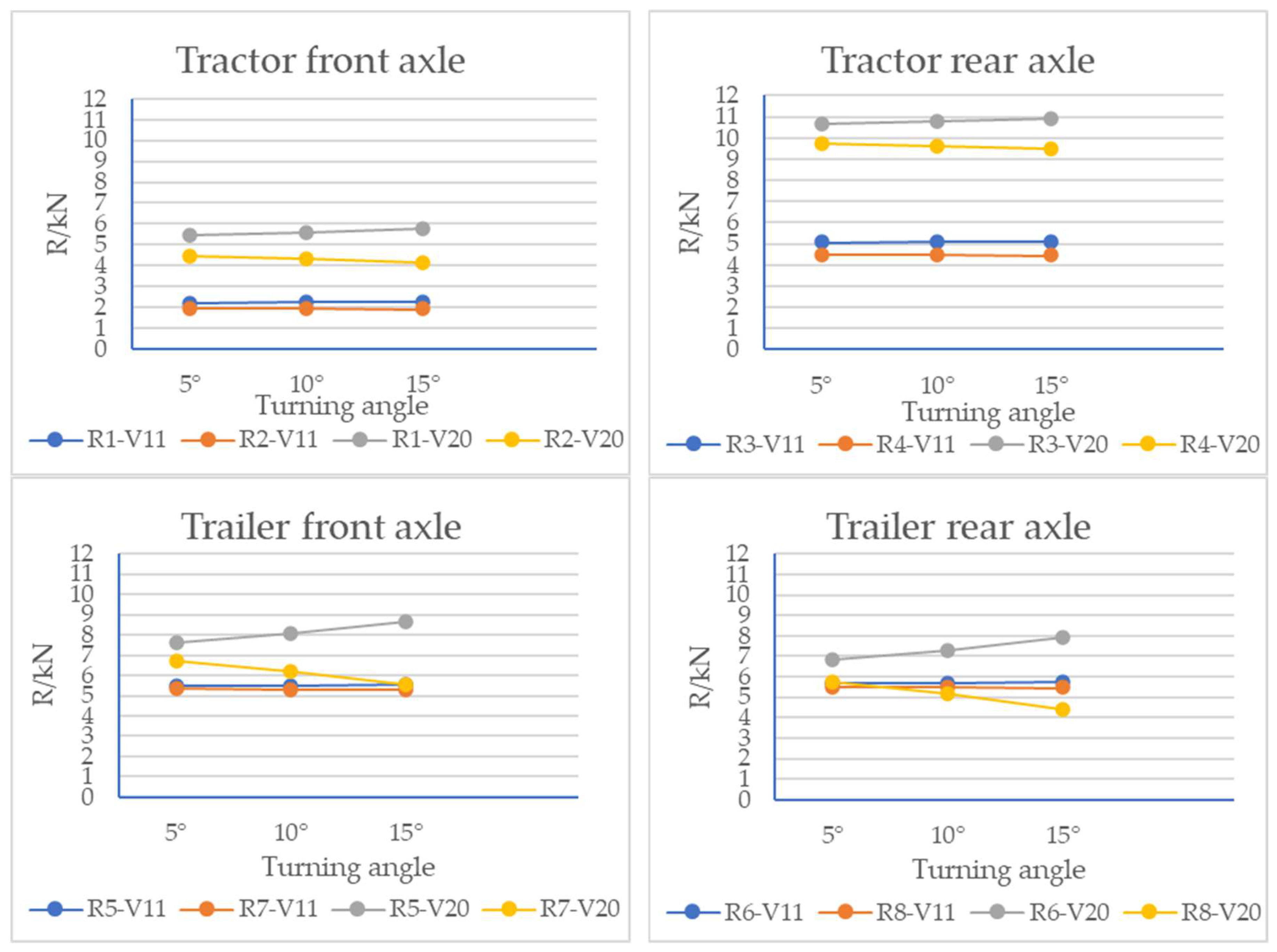
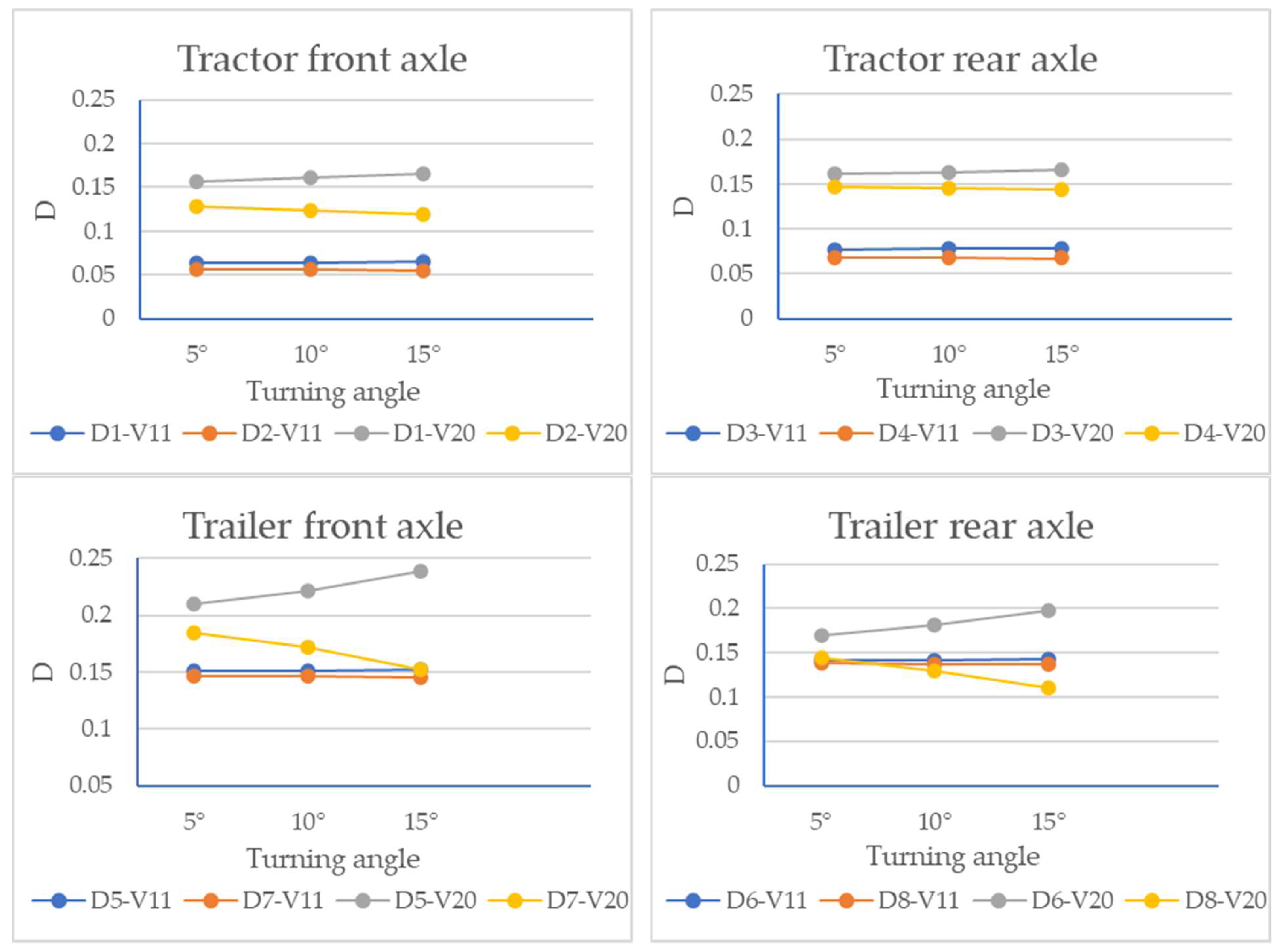
The root-mean-square value of the dynamic load and the dynamic load coefficient of each axle wheel of the four-axle vehicle are shown in Figure 21 and Figure 22.

The figures show the following:

• Similar to the situation of the three-axle vehicle, the faster the speed, the greater the dynamic load index of the vehicle.
• In cornering, the dynamic load indices of the left wheels of the tractor and the trailer are greater than those of the right wheel, and the dynamic load index of the left wheel gradually increases with an increase in cornering angle, while that of the right wheel steadily declines. The increase and decrease ranges are greater than those of the three-axle vehicle.

5. Conclusions

The excitation equation of a vehicle in contact with the pavement surface was established using the filtered white noise method, and an excitation model of all tires in contact with the pavement surface was obtained by combining the coherence function of the left and right wheels of the vehicle and the hysteresis of the front and rear wheels. According to the vibration dynamics theory, the vibration models of a three-axle vehicle and a four-axle vehicle are established, and the following conclusions can be obtained by simulating and investigating the changes in dynamic load indices under different conditions of pavement surface roughness, load, vehicle speed, and cornering radius.

• With a deterioration in the pavement roughness from grade A to grade D, the dynamic load of each wheel of the three-axle and four-axle vehicle increased nonlinearly, indicating that the greater the fluctuation in the longitudinal section of the pavement, the more intense the vibration generated by the wheel. Specifically, the average dynamic load increased by 95.3% when the roughness rose from grade A to grade D. Under 20% overload conditions, the peak dynamic load increased by 23.7% compared to under a standard load. Moreover, the higher the vehicle speed, the greater the influence of the pavement surface roughness on the dynamic load. At the same time, the dynamic load of the rear axle wheels of the three-axle vehicle was greater than that of the front axle and the intermediate shaft, and the dynamic load of the tractor of the four-axle vehicle was greater than that of the trailer.
• With the progression from no-load to overload, the root-mean-square value of the dynamic load of the three-axle vehicle first increased slowly and then gradually decreased with an increase in load, and the dynamic load coefficient showed a downward trend with an increase in load; similar characteristics were observed for the four-axle vehicle. This shows that an increase in load inhibited the vibration of the vehicle. At the same time, the dynamic load coefficient of the rear axle wheel of the three-axle vehicle was greater than that of the front wheel, and the dynamic load coefficient of the trailer wheel of the four-axle vehicle was greater than that of the tractor, which was related to the fact that the load weight was mainly concentrated in the rear compartment of the vehicle.
• As the vehicle speed increased from 6 m/s to 25 m/s, the dynamic load on the intermediate axle rose from 3894 N to 6261 N (a 60.8% increase), whereas the front axle load increased from 3807 N to 9396 N (a 146.8% increase), revealing significant differences in sensitivity to speed among different axle positions. The root-mean-square value of the dynamic load of the wheel of the three-axle vehicle increased first and then tended to become flat or decreased, and the dynamic load coefficient gradually increased for the front axle, while it first increased and then decreased for the intermediate shaft and the rear axle. The front axle of the tractor and the front and rear axle wheels of the trailer of the four-axle vehicle showed an increasing trend, while the rear axle wheels of the trailer showed a decreasing trend. Notably, when the vehicle’s vibration frequency (1.2–1.8 Hz) approached the dominant pavement excitation frequency (1.5 Hz), the dynamic load increased by up to 37.5%. This reflects the interaction between the vibration frequency of the vehicle and the excitation frequency of the pavement surface, and the negative influence on the pavement structure should be given great attention when the vehicle is driving at low speed.
• When the vehicle was in lateral tilt, the turning radius had a greater influence on the dynamic load index of the left and right wheels, and generally, the dynamic load index of the left wheel was greater than that of the right wheel, which was mainly caused by the centrifugal force of the vehicle’s cornering.

This study not only systematically revealed the evolution law of random dynamic loads for multi-axle heavy-duty vehicles under complex operating conditions but also provided a foundation for future research. Subsequent work could involve collaboration with transportation authorities to collect real-world WIM (Weigh-in-Motion) data for model validation under actual traffic conditions. Furthermore, pavement fatigue damage prediction tools can be developed based on the findings of this study, and the model can be extended to non-stationary road conditions, such as curves and slopes, to investigate dynamic load characteristics under complex driving scenarios, thereby supporting more accurate and durable asphalt pavement structural design.

References

1. Zhou, H.F.; Jiang, J.Q.; Mao, G.H. Analysis of Dynamic Vehicle Load Caused by Pavement Roughness. China Munic. Eng. 2002, 4. [Google Scholar] [CrossRef]
2. Dodds, C.J.; Robson, J.D. The description of road surface roughness. J. Sound Vib. 1973, 312, 175–183. [Google Scholar] [CrossRef]
3. Cebon, D. Theoretical road damage due to dynamic tyre forces of heavy vehicles part 1: Dynamic analysis of vehicles and road surfaces. Proc. Inst. Mech. Eng. Part C J. Mech. Eng. Sci. 1988, 202, 103–108. [Google Scholar] [CrossRef]
4. Watts, G.R. The generation and propagation of vibration in various soils produced by the dynamic loading of road pavements. J. Sound Vib. 1992, 156, 191–206. [Google Scholar] [CrossRef]
5. Deng, X. Study on dynamics of vehicle-ground pavement structure system. J. Southeast Univ. (Nat. Sci. Ed.) 2002, 32, 474–479. [Google Scholar] [CrossRef]
6. Naraghi, M.; Zadeh, E.N. Effect of Heavy Vehicle Suspension Designs on Dynamic Road Loading—A Comparative Study. SAE Int. Truck. Bus Meet. Expo. 2002, 110, 363–369. [Google Scholar]
7. Mitschke, M. Influence of Road and Vehicle Dimensions on the Amplitude of Body Motions and Dynamic Vehicle Loads. SAE Tech. Pap. 1962, 70, 434–446. [Google Scholar] [CrossRef]
8. Jing, C. Basic Research on the Interaction Between Vehicle and Pavement. Doctoral Dissertation, Jilin University, Changchun, China, 2002. (In Chinese). [Google Scholar]
9. Sun, L.; Luo, F. Nonstationary Dynamic Pavement Loads Generated by Vehicles Traveling at Varying Speed. J. Transp. Eng. 2007, 133, 252–263. [Google Scholar] [CrossRef]
10. Sayers, M.W.; Gillespie, T.D.; Queiroz, C.A.V. The International Road Roughness Experiment: Establishing Correlation and Standard for Measurements. In World Bank Technical Paper; The World Bank: Washington, DC, USA, 1986; Available online: http://documents.worldbank.org/curated/en/326081468740204115 (accessed on 1 July 2010).
11. Zhong, Y.; Wang, Z.R.; Zhang, X.N. Random Dynamic Pressure of Moving Vehicle on Rough Pavement. China J. Highw. Transp. 1992, 5, 40–43. (In Chinese) [Google Scholar]
12. Tao, X.; Hang, X. Analysis and calculation of frequency domain simulations of dynamic load. J. Huazhong Univ. Sci. Technol. Urban Sci. Ed. 2003, 20, 47–50. [Google Scholar]
13. Tan, R.H.; Chen, Y.; Lu, Y.X. The mathematical models in time domain for the road disterbances and the simulation. China J. Highw. Transp. 1998, 11, 96–102. [Google Scholar]
14. Ruichen, J. Simulation of the road irregularity and study of nonlinear random vibration of the automobile. J. Tsinghua Univ. 1999, 39, 76–79. [Google Scholar]
15. Hao, X.; Jun, X.; Xu, T. Influence analysis of driving dynamic load of multi-axle heavy-duty vehicles based on pavement roughness. J. Transp. Sci. Eng. 2023, 39, 26–37. (In Chinese) [Google Scholar]
16. Beskou, N.D.; Hatzigeorgiou, G.D.; Theodorakopoulos, D.D. Dynamic inelastic analysis of 3-d flexible pavements under moving vehicles: A unified fem treatment. Soil Dyn. Earthq. Eng. 2016, 90, 420–431. [Google Scholar] [CrossRef]
17. Si, L.T. Random Vibration Analysis of Linear Continuous Systems Under Moving Random Loads. Ph.D. Dissertation, Dalian University of Technology, Dalian, China, 2017. [Google Scholar]
18. Lv, Y.; Ying, B.; Zou, L. Stress-strain analysis of asphalt pavement under random loading. Highw. Eng. 2018, 43, 94–101. [Google Scholar]
19. Mamlouk, M.S. General outlook of pavement and vehicle dynamics. J. Transp. Eng. 1997, 123, 515–517. [Google Scholar] [CrossRef]
20. Fryba, L. Dynamic interaction of vehicles with tracks and roads. Veh. Syst. Dyn. 1987, 16, 129–138. [Google Scholar] [CrossRef]
21. Liang, B.; Su, S.Y.; Luo, H. Coupled dynamic analysis of vehicle-road system under roughness conditions. Eng. Mech. 2009, 26, 189–194. [Google Scholar]
22. Li, H.Y.; Yang, S.P.; Qi, Y.Q.; Xu, B.Q. Dynamics of asphalt pavement under moving stochastic loads and parameter analysis. Eng. Mech. 2011, 28, 159–165. [Google Scholar] [CrossRef]
23. Zhao, M.J.; Yin, T.; Fu, S.J. Dynamic response analysis and crack location of cracked beams considering the randomness of moving loads. Chin. J. Civ. Eng. Manag. 2016, 33, 102–108. [Google Scholar]
24. Dong, Z.; Ma, X. Analytical solutions of asphalt pavement responses under moving loads with arbitrary non-uniform tire contact pressure and irregular tire imprint. Road Mater. Pavement Des. 2018, 19, 1887–1903. [Google Scholar] [CrossRef]
25. Zeng, F.; Chen, F.; Eghbal, S. Vibroacoustic analysis of asphalt pavement responses to moving loads and attached mass-spring-damper systems. Soil Dyn. Earthq. Eng. 2024, 185, 13. [Google Scholar] [CrossRef]
26. Mo, C.L. Analysis of dynamic response of asphalt pavement structure and vehicle comfort. West. Transp. Technol. 2023, 7, 44–47. [Google Scholar] [CrossRef]
27. Luo, R.K.; Gabbitas, B.L.; Brickle, B.V. Fatigue Life Evaluation of a Railway Vehicle Bogie Using an Integrated Dynamic Simulation. Proc. Inst. Mech. Eng. Part F J. Rail Rapid Transit 1994, 208, 123–132. [Google Scholar] [CrossRef]
28. Cascino, A.; Meli, E.; Rindi, A. Comparative Analysis and Dynamic Size Optimization of Aluminum and Carbon Fiber Thin-Walled Structures of a Railway Vehicle Car Body. Materials 2025, 18, 1501. [Google Scholar] [CrossRef] [PubMed]
29. Xiandong, L. Research on the method of simulating road roughness numerically. J. Beijing Univ. Aeronaut. Astronaut. 2003, 29, 843–846. [Google Scholar] [CrossRef]
30. Yu, Z.S. Automobile Theory, 3rd ed.; China Machine Press: Beijing, China, 2004. (In Chinese) [Google Scholar]
31. Robson, J.D. Road surface description and vehicle response. Int. J. Veh. Des. 1979, 1, 25–35. [Google Scholar] [CrossRef]
32. Zhang, G.; Fang, Z.; Chen, S.; Song, Y. White Noise Simulation for Road Roughness Based on Power Function. Automot. Eng. 2008, 30, 44–47. [Google Scholar] [CrossRef]
33. Wang, Y.; Chen, S.Z.; Zheng, K.F. Simulation research on time domain model of road roughness with time-space correlation. J. Vib. Shock. 2013, 32, 70–74. [Google Scholar]
34. Lu, F.; Chen, S.Z. Modeling and simulation of road surface excitation on vehicle in time domain. Automot. Eng. 2015, 37, 549–553. [Google Scholar]
35. Zhou, C.; Sun, B.; Sun, Q.; Chen, N.; Ma, Z.; Li, S.; Wang, H. Modeling and simulation of harshness of an articulated tipper. Automob. Technol. 2004, 9, 15–18. [Google Scholar] [CrossRef]
36. Cole, D.J.; Cebon, D. Modification of a heavy vehicle suspension to reduce road damage. Proc. Inst. Mech. Eng. Part D J. Automob. Eng. 1995, 209, 183–194. [Google Scholar] [CrossRef]
Figure 1. Wheel pavement excitation of two-axle vehicle.
Applsci 15 09906 g001
Figure 2. Vibration model of three-axle whole vehicle. where m1—body mass, kg; mA; mB—unsprung mass (the weight supported by the elastic elements in the non-suspension system) of front axle, kg; mC1; mD1—unsprung mass of intermediate shaft, kg; mC2; mD2—unsprung mass of rear axle, kg; KtA; KtB; KtC1; KtC2; KtD1; KtD2—tire stiffness, N/m; CtA; CtB; CtC1; CtC2; CtD1; CtD2—tire damping coefficient, Ns/m; KSA; KSB; KSC; KSD—stiffness of suspension spring, N/m; CSA; CSB; CSC; CSD—damping coefficient of suspension, Ns/m; J1; J2; J3—pitching moment of inertia of body and balance suspension, kg·m2; θ1; θ2; θ3—pitching angle of body, balance suspension, rad; I—lateral tilt moment of inertia of the body, kg·m2; φ—Lateral tilt angle of the body, rad; ZA; ZB—vertical displacement of the unsprung mass of the front axle, m; ZC1; ZD1—vertical displacement of the unsprung mass of the intermediate shaft, m; ZC2; ZD2—vertical displacement of the unsprung mass of rear axle, m; Z1—vertical displacement of the body, m; Z1A; Z1B; Z1C; Z1D—vertical displacements at the four vertices of the body when the pitch angle θ and lateral tilt angle φ are small, m; qA; qB; qC1; qC2; qD1; qD2—pavement surface roughness excitation of each wheel, m; FA; FB; FC; FD—force of right front, left front, right rear, left rear suspension, N; a; b—distance from the front wheel center and rear axle suspension center to the body center of mass, m; l —wheelbase, m; d —length of balance suspension, m.
Applsci 15 09906 g002
Figure 3. Vibration model of four-axle whole vehicle. Where m1; m2; m3; m4—unsprung mass of the tractor, kg; m5; m6; m7; m8—unsprung mass of the trailer, kg; m9—sprung mass (the mass part supported by the elastic elements of the suspension system) of the tractor, kg; m10—sprung mass of the trailer, kg; K1; K2; K3; K4; K5; K6; K7; K8—tire stiffness, N/m; C1; C2; C3; C4; C5; C6; C7; C8—tire damping coefficient, Ns/m; K9; K10; K11; K12; K13; K14—stiffness of the suspension spring, N/m; C9; C10; C11; C12; C13; C14—damping coefficient of the suspension, Ns/m; J1; J2; J3; J4—pitching moment of inertia of the tractor, trailer, and balance suspension, kg·m2; θ1; θ2; θ3; θ4—pitching angle of tractor, trailer, and balance suspension, rad; I1; I2—lateral tilt moment of inertia of tractor, trailer, kg·m2; φ1; φ2—lateral tilt angle of tractor and trailer, rad; Z1; Z2; Z3; Z4—vertical displacement of the unsprung mass of the tractor, m; Z5; Z6; Z7; Z8—vertical displacement of unsprung mass of trailer, m; Z9—vertical displacement of the tractor body, m; Z10—vertical displacement of the trailer body, m; Z11; Z12; Z21; Z22; Z31; Z32—vertical displacements at the six vertices of the body when the pitch angles θ1; θ2 and lateral tilt angles Φ1; Φ2 are small, m; q1; q2; q3; q4; q5; q6; q7; q8—pavement surface roughness excitation of each tire, m; F1; F2; F3; F4; F5; F6—force of each suspension, N; a1; a2; a3—distance from the front axle of the tractor, hinge joint, and rear axle of the tractor to the center of mass of the tractor, m; b1; b2—distance from hinge joint, balance suspension to center of mass of the trailer, m; l—wheelbase, m; d—length of balance suspension, m.
Applsci 15 09906 g003
Figure 4. Vehicle model of lateral tilt. Where: m—sprung mass, kg; m1; m2—unsprung mass of left and right wheel, kg; K1; K2—stiffness of left and right suspension spring, N/m; K11; K21—stiffness of left and right tire, N/m; C1; C2—damping coefficient of left and right suspension, Ns/m; C11; C21—damping coefficient of left and right tire, Ns/m; Z—displacement of body center of mass, m; β—lateral tilt angle of the body, rad; Z2; Z3—vertical displacement of unsprung mass of front and rear axle, m; Z11; Z12—vertical displacements at the four vertices of the body when the pitch angle is small, m; l—wheelbase of the left and right wheel, m; I—rotational inertia of the body around the center of mass, kg·m2; q1; q2—pavement surface roughness excitation of front and rear wheel, m.
Applsci 15 09906 g004
Figure 5. Time-domain curves of dynamic load of three-axle vehicle.
Applsci 15 09906 g005aApplsci 15 09906 g005b
Figure 6. Time-domain curves of dynamic load of four-axle vehicle.
Applsci 15 09906 g006aApplsci 15 09906 g006bApplsci 15 09906 g006c
Figure 7. Trend of RMS’ variation with the grade of pavement roughness for three-axle vehicle.
Applsci 15 09906 g007
Figure 8. Trend of D’s variation with the grade of pavement roughness for three-axle vehicle.
Applsci 15 09906 g008
Figure 9. Trend of RMS’s variation with the grade of pavement roughness for four-axle vehicle.
Applsci 15 09906 g009
Figure 10. Trend of RMS’ variation with the grade of pavement roughness for four-axle vehicle.
Applsci 15 09906 g010
Figure 11. Trend of RMS’ variation with load for three-axle vehicle.
Applsci 15 09906 g011
Figure 12. Trend of D’s variation with the load for three-axle vehicle.
Applsci 15 09906 g012
Figure 13. Trend of RMS’ variation with load for four-axle vehicle.
Applsci 15 09906 g013
Figure 14. Trend of D’s variation with load for four-axle vehicle.
Applsci 15 09906 g014
Figure 15. Trend of RMS’ variation with speed for three-axle vehicle.
Applsci 15 09906 g015
Figure 16. Trend of D’s variation with speed for three-axle vehicle.
Applsci 15 09906 g016
Figure 17. Trend of RMS’ variation with the speed for four-axle vehicle.
Applsci 15 09906 g017
Figure 18. Trend of D’s variation with the speed for four-axle vehicle.
Applsci 15 09906 g018
Figure 19. Trend of RMS’ variation with turning angle for three-axle vehicle.
Applsci 15 09906 g019
Figure 20. Trend of D’ variation with turning angle for three-axle vehicle.
Applsci 15 09906 g020
Figure 21. Trend of RMS’ variation with turning angle for four-axle vehicle.
Applsci 15 09906 g021
Figure 22. Trend of D’s variation with turning angle for four-axle vehicle.
Applsci 15 09906 g022