Abstract
This paper addresses the challenge of stabilizing an unmanned aerial vehicle with an arm (UAM) on a pipeline with disturbance, where the disturbance factors include white noise, mass uncertainty, and wind disturbance. An anti-disturbance control method is proposed utilizing nonlinear model predictive control (NMPC). Initially, the natural wind field model is developed. Considering wind disturbance, the UAM dynamics are analyzed utilizing Newton–Euler theory. Subsequently, the no-slip constraints and the terminal constraints are defined to prevent UAM from destabilizing and falling. The NMPC-based algorithm is developed to ensure the stable control of UAM, transforming the optimization problem into a nonlinear programming problem. The terminal cost function and the inequality constraints for establishing the state variables using linear quadratic regulator (LQR) are meticulously studied. Finally, numerical simulations are carried out to further verify the proposed method, considering internal disturbance about physical parameters and external disturbance about wind. Simulation results show that the disturbance is well compensated, and the UAM tilt angle is less than 0.3 deg. Therefore, the proposed control method can comprehensively consider the input energy consumption and the realization of stability, and has a certain degree of anti-interference.
1. Introduction
In recent years, unmanned aerial vehicles (UAVs) have been widely employed in the fields of military reconnaissance, aerial photography, industrial inspection, fire search and rescue, geographic information collection scenarios, etc. [1]. This is owing to their advantages of simple structure, low maintenance costs, and the ability to hover vertically. As the technology continues to progress, the application of UAVs expands, attracting a large number of scholars [2]. The pipeline inspection is an important application field of UAV [3]. Pipelines are important in-plant transmission equipment for chemical materials like oil and gas. With the accumulation of service life, the pipelines encounter problems of perforation and oil leakage. It is necessary to carry out regular maintenance on transmission pipelines. However, a series of challenges appears during maintenance. Terrain complexity and variability significantly increase the difficulty of maintenance. Furthermore, technical limitations and operational complexity lead to inefficiencies [4]. These issues must be addressed to ensure the safe and efficient operation of chemical production.
As an alternative to human inspection of transmission pipelines, the UAM can significantly improve the efficiency and safety of the inspection process. Compared with traditional manual inspection methods, the UAM inspection omits building special inspection channels, thus realizing fast and comprehensive inspection. Furthermore, it not only conserves time and human resources but also markedly enhances the operational safety of the process. In addition, timely detection of hidden dangers effectively prevents safety incidents and high maintenance costs, which may be caused by pipeline leakage [5].
It is noteworthy that the UAM system [6] has the following characteristics, including inherent mass parameter uncertainty, underdrive characteristics, highly nonlinear dynamics, strong coupling between the robotic arm and the UAV system. The characteristics lead to complex control challenges. Furthermore, uncertain interference factors from the external environment exacerbate the difficulty of controlling UAM on the pipeline. The stability of UAM on the pipeline is the premise of subsequent inspection operations. This technology also provides important references for various pipeline detection applications, such as fire water pipeline and power line detection.
Currently, the inspection of transmission pipelines performed by drones is mainly a non-contact operation. The UAV hovers over the pipeline and collects data such as temperature and pressure using sensors such as cameras and thermal imagers. Subsequently, image recognition techniques are used to detect pipeline anomalies [7]. In [8], a quadcopter UAV is employed for oil pipeline monitoring, and a PID controller is designed to control the distance between the quadcopter UAV and pipeline. In [9], a UAV equipped with non-contact sensors is studied for inspection of oil and gas pipelines. An image processing technology is proposed to realize autonomous navigation and pipeline tracking. This hovering inspection mechanism has limited detection accuracy. Tiny cracks are usually not found in time. During the inspection process, the UAV is unable to make direct contact with the pipeline due to its non-contact operational characteristics. As a result, it is unable to directly and accurately obtain data on key parameters such as pressure and temperature inside the pipeline. This limitation may lead to an imprecise assessment of the pipeline condition, which in turn affects the accuracy of the inspection results.
The wheels of UAM can adhere to pipelines and move freely along them, reducing power consumption caused by propeller rotation during hovering in non-contact inspection processes. There are fewer studies on UAV contact inspection, and such studies can be analogized to different adsorption mechanisms for high-altitude robots. Zhou et al. [10] utilize the air rotation inertia effect to generate adhesion force, enabling the robot to climb walls with various roughness levels. Fan et al. [11] addresses the issue of insufficient magnetic adhesion leading to poor robot locomotion performance. The mechanism of electromagnetic and internal force compensation is proposed to achieve reliable adhesion functionality. Zhu et al. [12] adopts vacuum adhesion, aligning the suction cups of a bipedal wall-climbing robot with the target surface to form a sealed space, ensuring that the robot does not fall during the climbing process.
During UAM operations conducted at elevated altitudes, wind disturbances are inevitable and significantly impact the stability of the system. Therefore, it is imperative to thoroughly consider and effectively address wind disturbance factors by selecting appropriate control methodologies to ensure the stability of the system. The presence of wind disturbances exacerbates the nonlinearity of the system dynamics. In [13], radial basis function neural networks (RBFNNs) are utilized to estimate unknown nonlinear functions. By integrating the adaptive neural controller (-ANC) with the -based adaptive neural sliding mode controller (-ANSMC), helicopter trajectory tracking under wind disturbance conditions is achieved. In [14], the Dryden model is used to establish a turbulent wind field model. A dual-loop control scheme for a quadrotor aircraft is proposed, incorporating active disturbance rejection control (ADRC) and linear disturbance rejection control (LADRC). The outer loop is designed to mitigate wind disturbance, while the inner loop is responsible for tracking the desired trajectory. In [15], a two-stage particle filter is employed to estimate information regarding external wind disturbances. A non-singular terminal sliding mode control (NTSMC) strategy is devised for the purpose of wind disturbance. The adaptive drag coefficient is used to generate a compensation control signal to reduce the estimation error caused by wind disturbance. To further augment the system’s anti-disturbance capability, Zhang et al. [16] introduces an extended state observer (ESO) for real-time estimation and compensation of disturbances. Additionally, Wang et al. [17] design finite-time disturbance observers to observe wind disturbance. Meanwhile, a non-singular terminal sliding mode control strategy is proposed to ensure that the tracking error converges to zero within a finite time frame.
NMPC is favored in academic research and engineering practice for its robustness properties [18,19]. Rolling time-domain optimization guarantees adaptation to model parameter changes and ensures stable system performance, and is widely used in nonlinear system control [20,21]. In [22], a controller is developed for trajectory tracking control of a small helicopter. The controller is bases on the Explicit Nonlinear MPC (ENMPC) and the Disturbance Observer-Based Control (DOBC). The proposed controller improves the shortcoming of NMPC requiring a large amount of online computation. Moreover, the disturbance observer can accurately estimate the wind disturbance and modeling error to achieve ideal tracking. In order to solve the tire slip problem within complex road environments, the steering angle limit and tire adhesion area bounds of Unmanned Ground Vehicles (UGVs) are studied utilizing MPC in [23]. The NMPC, developed in [24], effectively addresses the challenges of flight envelope with extreme maneuvering scenarios.
The above study shows that there are few contact inspections for UAM. Given this, how to keep the UAM stable on the pipeline in the presence of quality parameter uncertainties and external wind disturbances is the key issue in this paper [25]. In order to cope with the above challenges, this paper proposes an NMPC-based anti-disturbance control method for UAM. The method ensures that the UAM is quickly and stably on the transmission pipeline under the environment of external wind disturbance.
The paper is structured as follows. Section 2 presents the dynamic model of UAM considering wind disturbance. In Section 3, the design of the NMPC algorithm is presented, along with the specified constraints. Furthermore, a stability analysis is conducted. In Section 4, the external disturbance and internal disturbance are considered and the numerical simulation is carried out. Finally, Section 5 concludes the paper. The innovativeness of this paper can be summarized with the following three points:
- 1.
- A contact inspection mechanism of UAM is proposed for the inspection of aerial transmission pipelines in chemical plants, improving accuracy of the traditional non-contact mechanism and reducing power loss generated by UAM hovering.
- 2.
- The external wind field is taken as a disturbance variable, which is integrated into the UAM dynamics for the first time, so as to obtain the dynamics model of UAM considering wind disturbance factor. The establishment of this model provides strong support for accurately describing the dynamics of the UAM under the wind disturbance.
- 3.
- Based on the dynamics model of UAM with wind disturbance factor, the no-slip constraints are designed utilizing mechanical analysis and the law of friction. An NMPC-based strategy is developed to stabilize the UAM system. Terminal domains and terminal penalties are designed to guarantee the stability of the system.
2. Dynamic Model of UAM Under Wind Disturbance
In this work, the UAM consists of a lightweight robotic arm and a wheeled X-type quadrotor UAV. The UAM combines the free-flying characteristics of UAV with the flexibility of the arm. The UAV is equipped with two driving wheels and two gimbals. The robotic arm is mounted directly on the UAV and is composed of light and high-strength materials, which can be freely expanded and change direction. To minimize power loss during hovering, the four wheels, equipped with navigation and localization devices, are able to travel freely along the pipeline. The system is powered by the rotation of four propellers and the torque generated by the wheels in contact with the pipeline. When the wheel torque reaches saturation, the rotation of the propellers will provide the required power to UAM. The underside of UAM is equipped with a tilt sensor. Through the integration of internal accelerometers and gyroscopes, the tilt angle of UAM relative to the pipeline can be accurately measured. The data processing unit processes the detected inclination data and transmits it to the controller. The components work together to eventually stabilize the UAM on the pipeline. Figure 1 illustrates a schematic of UAM on the transmission pipeline. The UAM consists of a UAV and an arm. The UAM lands on a horizontal pipeline to perform the pipeline measurements or other required tasks. Due to the geometric shape of the pipeline, the UAM landing is not exactly on the top of the pipeline. Furthermore, during the UAM navigation on the pipeline, the disturbance factors affect the UAM motion. Therefore, it is a pre-requisite to stabilize the UAM system on the pipeline.
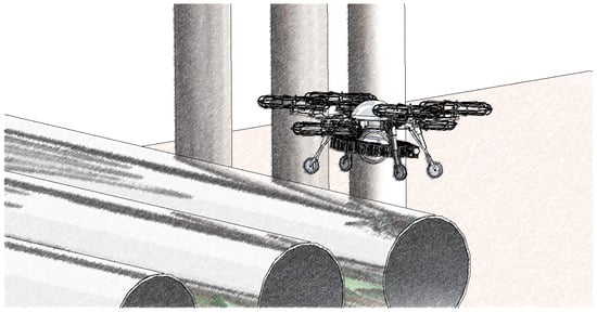
Figure 1.
Schematic of UAM on the transmission pipeline [26].
The aim of this paper is to simulate the real environment in which the UAM works. The problem of stabilizing the UAM on the transmission pipe in a wind-disturbed environment is investigated [27]. The UAM system is not stabilized at the moment of landing on the transmission pipe. Furthermore, the robotic arm remains motionless. There is no effect on the center of gravity of the UAM.
2.1. Wind Disturbance Models
In order to simulate the real working environment of UAM, the wind field model is constructed. Natural wind has the characteristics of randomness, suddenness, persistence and periodicity [28]. Therefore, the natural wind can be classified into four types, including continuous wind, gust wind, gradual wind and random wind [29].
For continuous wind, the wind speed is constant and is expressed as:
For gust wind, the wind speed is generated at a certain moment suddenly and is gradually strengthened. After a period of time, decreases until it disappears. The gust wind usually changes periodically and the Discrete Gust Model is selected to simulate the gust wind [30], calculated as:
For gradual wind, the wind speed gradually changes over time, while not suddenly becoming smaller or larger. The formulation of is as follows:
For random wind, the wind speed does not change regularly with time. The character of random wind is its randomness [31], including the generation, the disappearance, the increase and the decrease. is formulated as:
In above equations, denotes the coefficient for continuous wind speed. , and are, respectively, the maximum wind speeds of gust, gradual wind and random wind. and , respectively, indicate the start time and the period of gust. and , respectively, indicate the initial and the final time instants where the gradual wind speed varies. indicates a random number uniformly distributed from −1 to 1, indicates the frequency of random wind, and indicates a random component in the range of .
By weighting and summing the above four winds with different proportional weights, the natural wind speed is constructed as:
where is the weight coefficient of each type of wind, satisfying . The force of wind disturbance is calculated as:
where indicates the force of wind disturbance, and indicates the UAM drag coefficient. , where C denotes the air drag coefficient, and S denotes the windward area. indicates the air density, and V indicates the relative air speed. This paper focuses on the moment the UAM lands on the pipeline; the UAM velocity is negligible. Therefore, V also indicates wind speed.
2.2. Dynamic Model of UAM with Wind Disturbance
The physical interaction dynamics between UAM and the pipeline is studied in this part, integrating the influence of external wind disturbance. During the UAM system performing tasks on the pipeline, the following assumptions are considered.
- (1)
- The UAM system is designed as a homogeneous and symmetrical rigid structure. The transmission pipeline has the same rigid qualities and does not produce any deformation during operation. The Coulomb friction law is employed to analyze the static friction between the UAM wheels and pipe. Since the sliding friction force is much less than the static friction force, the rolling friction is negligible.
- (2)
- The connection point between UAV and the robotic arm coincides with the center of mass of UAM. The robotic arm does not work before the UAM system comes to a steady state on the pipe, reducing the difficulties of controlling the UAM system while having no influence on modeling the UAM system.
- (3)
- The inertial effects of UAM wheels and propellers are neglected. Furthermore, the wheels are assumed not to slip on the pipeline.
- (4)
- Both the UAM wheels and propellers are fixed at a specific position. The fixed position of propellers contributes to the combined effect of UAM. The barycenter is always parallel to the tangent to the pipe.
- (5)
- The direct interference of wind on the propeller is ignored, and only the wind disturbance at the center of mass of UAM is considered.
Based on aforementioned assumptions, the resulting system is derived. Since the UAM is symmetric to the vertical plane cutting the system at its barycenter, a 2D depiction is utilized to further simplify the UAM dynamic model [32]. Figure 2 shows the 2D schematic diagram of UAM. The yellow part is the transmission pipeline. , and are the center of mass of UAM and the center of two wheels. denotes the force of wind disturbance, which is assumed to be at an angle from the horizontal line. denotes the angle of the line between the UAM center of mass and the center of the pipeline with respect to the -axis. The figure shows that the UAM reaches a steady state when and are 0.
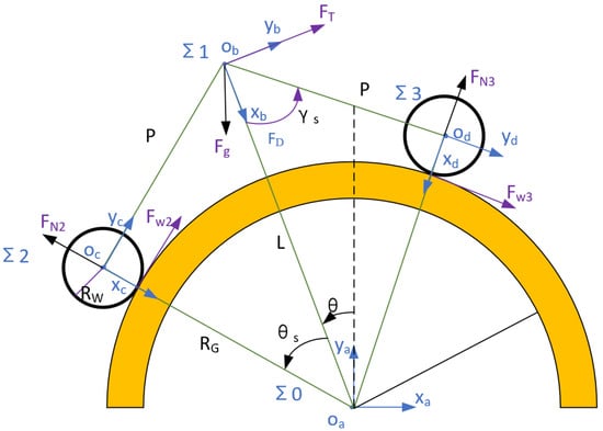
Figure 2.
Two-dimensional schematic diagram of UAM.
In order to facilitate the description of UAM dynamics, the following coordinate systems are established, namely the pipe center coordinate system : , the UAM center-of-mass coordinate system : , the two wheel coordinate system : , : . Since is the base coordinate system, the following formulations are derived.
where denotes the inclination angle of UAM on the pipe, namely the angle between line and line in Figure 2. indicates the angle between the line and . Under wind disturbance, the resultant force on UAM is expressed as follows:
where denotes the resultant force, denotes the gravitational force of UAM system, denotes the lateral thrust generated by rotation of propellers, and denote the tangential force due to the driving torque of two wheels. denotes the wind force, where the angle between the force and positive direction of axis is denoted as . The aforementioned force is formulated as follows:
where m is the UAM mass, g denotes the gravitational acceleration, , , , . denotes the two-fan number of force. and denote the driving torque of UAM wheels, and denotes the radius of UAM wheels.
According to aforementioned equations and combining the Newton–Euler formula , the dynamics model of the UAM system under wind disturbance is formulated as:
where L denotes the distance between the UAM center and the pipeline center, namely the length of line in Figure 2.
3. Nonlinear Model Predictive Control
The PID method can actually help to control the system without any disturbance. However, this paper focuses on the UAM control with external and internal disturbance; the performance of PID is not good. Since the UAM system has a physical interaction with the pipeline, the mathematical formulation is a nonlinear system with strong nonlinearity. Furthermore, the disturbance model is considered, making the system nonlinearity stronger. The performance of LQR is also not good. Therefore, an NMPC method is studied to control the stability of the UAM on the transmission pipeline under wind disturbance.
The block diagram of the NMPC system under wind disturbance is shown in Figure 3. First, the current state of UAM is input into the prediction model to obtain the future multi-step state vector under wind disturbance. Then, the objective function is constructed by combining the reference state and the control sequence. Taking full account of the system constraints, the objective function is solved within the control period to obtain the optimal control sequence that minimizes it. Only the first one is taken as the control input of the current UAM to obtain the state at the next moment. The next control cycle is entered and the rolling optimization is carried out continuously. Finally, the stability of UAM on the transmission pipeline is realized.
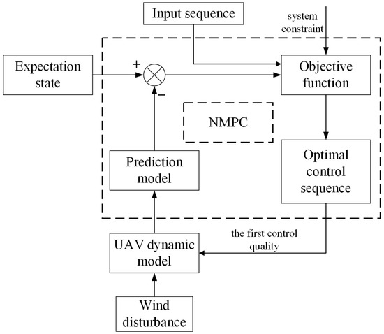
Figure 3.
Block diagram of NMPC system under wind disturbances.
NMPC has attracted much attention due to its ability to fully consider constraints of nonlinear systems [33,34,35]. The NMPC combines the reference state and predicts and in a certain time domain in the future according to a prediction model. Impose constraints on the system’s future inputs, control, and stabilization stopping conditions. Using this constraint, we construct an objective function incorporating control inputs and states, which defines the optimal control problem. By solving this problem, an optimal control sequence is obtained and the first value in the sequence is applied to the system. This process is carried out cyclically to achieve rolling optimization [36,37].
3.1. Predictive Model
According to Equation (12), the state space equations of the UAM system can be obtained as:
where is a two-dimensional state vector, , is a three-dimensional control input vector, . In this paper, the system output is chosen to be equal to the state, namely .
Since analytical solutions of continuous systems are scarcely derived, it is necessary to discretize the continuous system. The state update equation of the discretized system is formulated as:
where is the sampling period, using the Eulerian discretization of Equation (13):
3.2. Restrictive Condition
3.2.1. Constraints on States and Inputs
In order to ensure the safety and the stability of the UAM on the pipeline, the lateral thrust and the wheel torque must be strictly controlled. Large thrust makes the system out of control, while small thrust leads to insufficient power. If the torque exceeds the threshold value, the UAM system slips. If the torque is not enough, the UAM system slides down. Furthermore, the initial inclined angle should be constrained to prevent the instability of the UAM on the pipeline.
3.2.2. No-Slip Constraints
According to reference [31,32] for walking robots, the resultant force must be inside the support polygon to ensure the UAM stability against gravity. Namely, the force must be within the cone of angle . Inspired by the Coulomb friction theory [32,33], the constraint can be formulated as:
Assumption (3) in Section 2.2 means that the wheels do not slip on the pipe, namely each wheel should satisfy the no-slip condition. It also means that the UAM system does not separate from the pipe during movement. The resultant force of each wheel can be decomposed along the tangential direction and the normal direction of the contact surface. According to the Coulomb friction theory [32,33], the tangential force on each wheel must be less than or equal to the maximum static friction applied:
where represents the friction coefficient between the wheels and the pipe, is the tangential force, and represents the normal force (). The problem is how to get the relation between and other involved forces. According to the moment equilibrium constraint, the following formulation is derived.
where P denotes the distance between the UAM and the pipe center. Based on the trigonometric law and combining Equations (7)–(9), (11) and (21), and are derived as follows:
According to the Coulomb theory and combining Equations (19), (20) and (22), the following formulation is derived.
Therefore, the no-slip condition can be expressed as:
3.2.3. Terminal State Constraints
Terminal state constraints are set to ensure that the UAM can eventually be stable on the transmission pipeline under wind disturbance:
The stabilized state is achieved in the case that both the inclined angle and inclined angular velocity are 0, where and are the state components at the final time instant.
3.3. Design of NMPC Algorithms
The design objective of the controller is not only to achieve good closed-loop performance, but also to minimize the sum of deviations. These deviations include those of the predicted state from the desired state and the predicted input from the desired reference input within the prediction time domain. The terminal cost function is considered to ensure the rolling feasibility and asymptotic convergence of the NMPC optimization problem.
NMPC solves constrained nonconvex nonlinear optimization problems at each sampling period. Combined with the practical situation, Equation (18) yields the initial state and control constraints of the system as:
Assuming that the state of the system in Equation (16) is fully measurable and there is no model mismatch, the system satisfies following constraints:
- (1)
- The mapping is continuous, and ;
- (2)
- is a tight and convex set, is a connected set, and the equilibrium point lies inside the set .
The NMPC optimal control problem at moment can be represented as:
where denotes the prediction interval and is chosen to be the same as the control interval.
The expression of the objective function is as follows:
where
and are the system state and the control input positive definite weight matrices, respectively. The minimization of the difference between the predicted state and desired state serves as one of the objectives for the optimization of the objective function. At the desired equilibrium point, the control input and the desired equilibrium state satisfy and . denotes the terminal cost function.
According to above considerations, the problem of stabilizing the UAM on the transmission pipeline is transformed into a feasible solution problem, where the optimization problem is shown in Equation (27). At each sampling period, the optimization problem is solved online based on the current system state to obtain the predicted system state and the allowed control input sequence. Subsequently, the first element of the optimized control sequence is selected as the actual control quantity. Upon entering the next sampling moment, the above process is repeated using the new measurement information.
3.4. Stability Analysis
For the NMPC optimal control problem at moment k, a terminal cost function is established to penalize the final state of finite horizons. In addition, The specific definitions of the feasible set, feasible control sequence, optimal value function, and optimal control sequence are described as follows [38].
Definition 1.
Considering the nonlinear optimal control problem in Equation (27) with the prediction interval , where denotes the set of non-negative integers, the specific form of the feasible set is defined as follows:
For any , define the set of feasible control sequences as:
where represents the set of control sequences.
Definition 2.
Considering the nonlinear optimal control problem in Equation (27) and the prediction interval , define the optimal value function as:
The control sequence is defined as the optimal control sequence of the nonlinear optimal control problem with as the initial value. If the optimal value function satisfies:
then the corresponding is called the optimal state sequence.
For the constraint set of the state variables, the cost function of the state variables in the terminal prediction interval, and the feasible control sequence set in the nonlinear control optimization problem in Equation (27), the following assumptions are established.
Assumption 1.
The state variable constraint is feasible, meaning that for each , there exists such that:
Assumption 2.
For each , there exists such that:
Lemma 1.
Consider the time interval , where . For the nonlinear optimal control problem in Equation (27), if there exists an optimal control sequence , then the NMPC feedback control law possesses the following properties:
where in Equation (27) denotes the subset of control sequence element domains corresponding to the first element in the control sequence .
Lemma 2.
Lemma 3.
For the nonlinear optimal control problem in Equation (27), assuming that Assumptions 1 and 2 hold, then for any initial state , the optimal value function possesses the following properties:
Lemma 4.
Let the NMPC sampling period be denoted by , and the prediction horizon by N. At each sampling instant , the NMPC feedback control law is denoted as , and the corresponding optimal control sequence of the nonlinear optimal control problem in Equation (27) is denoted as . Let the forward feasible set of the closed-loop system in Equation (14) be denoted as . If there exists a scalar such that the following inequality holds:
for all and , then:
Theorem 1.
Denote the NMPC sampling period as and the prediction interval as N. When solving the nonlinear optimal control problem at each sampling instant , if Assumptions 1 and 2 are satisfied, and the stage cost function and the optimal value function in Equation (27) satisfy the following inequalities:
where , then the closed-loop system under the NMPC feedback control law is asymptotically stable.
Proof.
From Equation (38) in Lemma 1 and Equation (39) in Lemma 3, it follows that for any , the following holds:
□
According to Lemma 2, the set is forward invariant. On the other hand, let , and assume that . Then the assumptions in Lemma 4 are satisfied, and hence Equation (41) holds. Therefore, the closed-loop system under the NMPC feedback control law is asymptotically stable.
Detailed proofs of Lemmas 1 to Lemma 4 and Theorem 1 are given in [38]. In order to further satisfy the assumptions in the theorem, it is necessary to construct the terminal cost function and inequality constraint . The linear quadratic regulator (LQR) is used to obtain the penalty matrix , and then and are constructed based on . Aiming at the sampling time , the following steps are given to construct , and .
Step 1: The system is linearized at the reference point and , as follows:
The coefficient matrices and are calculated as:
According to the specific parameters in Table 1, the eigenvalues of the solved coefficient matrix A are 4.9528 and −4.9528. Both eigenvalues lie outside the unit circle; thus, the system in Equation (45) is open-loop unstable. Since rank(B,AB) = 2 is full rank, the system in Equation (45) is fully controllable. Therefore, the unstable modes of the system are controllable, namely the system is stabilizable. Furthermore, there must be a linear feedback control law making the system asymptotically stable [39].

Table 1.
System and controller parameters.
Step 2: Solving the discrete algebraic Riccati equation in Equation (47) yields a penalty matrix with positive definiteness and duality.
Step 3: For the LQR problem, a feedback control law u satisfying Assumptions 1 and 2 is designed and applied to the system in Equation (43), where is formulated as follows:
The purpose of control law is exclusively to calculate and at the current sampling instant and does not act on the real system.
Step 4: Define , and . Calculate and according to Equation (49):
According to Equation (49), and are calculated. At each sampling time k, the optimal control problem is solved. the optimal solution at moment k is . By defining the feedback control law for NMPC, the system state at time k + 1 can be obtained. Based on the above, the closed-loop system based on the NMPC feedback control law is asymptotically stable.
4. Numerical Simulations
In this part, numerical simulations are carried out to verify the proposed anti-disturbance control of UAM utilizing NMPC. The fmincon function in MATLAB R2024a toolbox is chosen to solve the NLP problem of NMPC. Two cases are provided for further analysis. In case 1, the external disturbances are considered, namely the wind disturbance. In case 2, the internal disturbances are considered as well as external disturbances in case 1. In addition, white noise with a standard deviation of deg/s was added. The UAM modeling is based on the assumption that the system is a rigid structure. However, during real flight, the mass of UAM components vary due to abrasion. The corresponding moment of inertia and the center of mass position change. Therefore, the UAM physical parameters are changed [39]. This leads to a series of potential effects on UAM flight control. Therefore, the effect of mass parameter uncertainty must be taken into account; the internal disturbance is considered with 10% uncertainty of UAM mass [40,41].
The values of prediction interval N and sampling period affect the stability and the real-time performance of the UAM system. In each case, the optimal values of N and are selected through a series of experiments. The variation of system parameters at different initial tilt angles is observed. The system and controller parameters are shown in Table 1.
Inspired by the analysis in Wang et al. [29] and Cui et al. [30], the weighting coefficients , , , in Equation (5) are, respectively, set as 0.3, 0.3, 0.3, 0.4. Combined with Equation (6), the wind field force variation curve is constructed as shown in Figure 4, where the wind reaches its maximum of 5 N at 4.5 s.
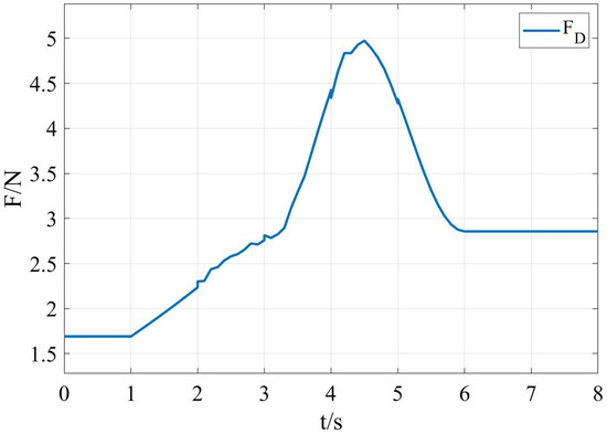
Figure 4.
Variation curve of wind disturbance force.
4.1. Case 1: Numerical Simulation with External Disturbance
4.1.1. Selection of Optimal Prediction Interval Length N
The initial tilt angle is set as , and the sampling period . The weighting matrices are empirically selected as , , so , , . In addition, the coefficient matrices A and B are valued as:
Generally, a large interval length N allows for a long prediction time horizon as well as high accuracy of the prediction model. As the value of N increases, the prediction performance of the controller is gradually improved. However, the computational complexity increases. In order to optimize the interval length N, the value of N is initially selected as 5, 6, 7, and 8. Figure 5 illustrates the variation curves of state variables, control inputs, and control constraints. The computational time is 118 s, 228 s, 264 s, 409 s, respectively.
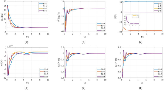
Figure 5.
Simulation results of case 1 with variable N, where (a,b) denote the response curves of the states, (c) denotes the four constraint satisfaction cases, and (d–f) denote the response curves of the inputs.
Figure 5a,b show the variations of state variables and , respectively. The state variable is in the range of 0°∼30°, meeting the constraints in Section 3.2 about state variables. The four curves in Figure 5c indicate the satisfaction of the constraints in Section 3.2, where , , , , , . The curves show that the constraints are satisfied, including the combined force, the friction, and the torques. Figure 5d–f denote the variation curves of , over time.
The wind disturbance is considered at the beginning of the simulation. At the time instant of 4 s, the system states and converge to desired values. Due to the wind disturbance at 4 s, the state curves tremble and the system is over-regulated. However, at 7 s, the curves tend to be stable again. Therefore, the designed controller can meet the requirements of stability. The lateral thrust and the torques and converge to stable values at about 8 s. Although the state curve converges fast when N = 8, the propeller lateral thrust is also compensated about . By balancing the adjustment time and the overshoot, the value of N is finally selected as N = 7.
4.1.2. Selection of Optimal Sampling Period
A large value of sampling period leads to inaccurate capture of system states, especially the case that the disturbance appears. Thus, the controller cannot adjust the deviation in a timely manner. A small makes the the sampling period intensive, and the computational burden increases. In order to optimize sampling period , the value of is initially selected as 0.01 s, 0.02 s, 0.03 s, and 0.04 s. The simulation results are shown in Figure 6, where N = 7 and . The computational time is 320 s, 232 s, 186 s, 126 s, respectively.
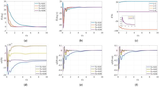
Figure 6.
Simulation results of case 1 with variable , where (a,b) denote the response curves of the states, (c) denotes the four constraint satisfaction cases, and (d–f) denote the response curves of the inputs.
Figure 6a shows that the state variable is in the range of 0°∼26°. The control inputs under the four different sets of sampling period all meet the constraints in Section 3.2. When is taken as 0.04 s, the tilt angle converges to 0 at the fastest rate and the regulation time is shorter compared to the other curves. However, the control input is compensated with . The tilt angle converges to the desired value most slowly when s. Furthermore, the control input is compensated with . Therefore, the sampling period is too short. The curve with the smallest input compensation and the fastest adjustment speed is selected, contributing to the optimal sampling period = 0.02 s.
4.1.3. Different Initial Tilt Angle
In this part, variable values of initial tilt angle are studied, based on the optimal prediction interval length N = 7 and the optimal sampling period = 0.02 s. The values of are selected as , .
Figure 7 shows the simulation results. The computational time is 225 s, 264 s, 184 s, 156 s, respectively. In Figure 7a,b, the system state variables converge to desired values 0. The four constraint curves in Figure 7c show that all the constraints in Section 3.2 are satisfied. As can be seen in Figure 7d, the UAM finally reaches steady states. The propeller lateral thrust is compensated with an input of 0.05 N when . However, the propeller lateral thrust is not compensated when . Therefore, a large initial tilt angle needs great compensation of propeller lateral thrust. This is due to the fact that the UAM centripetal force component decreases as increases. Furthermore, a large torque is required. Figure 7d–f show that the control input curves are symmetrically distributed over time with respect to the positive and negative initial tilt angles. Under the wind disturbance, both the control input and the state vector can be stabilized at about 7 s.
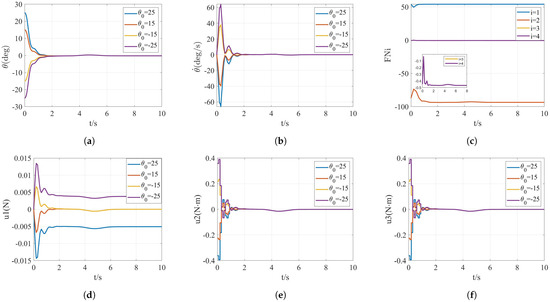
Figure 7.
Simulation results of case 1 with variable , where (a,b) denote the response curves of the states, (c) denotes the four constraint satisfaction cases, and (d–f) denote the response curves of the inputs.
In Figure 7, the tilt angles approach deg. The tilt angular velocities, respectively, approach deg/s, deg/s, deg/s and deg/s with initial tilt angles of 25 deg, 15 deg, −15 deg and −25 deg. The values of , respectively, approach 54.15, −93.53, −0.47 and −0.47. The values of input , respectively, approach N, N, N and N with initial tilt angles of 25 deg, 15 deg, −15 deg and −25 deg. The values of input , respectively, approach N · m, N · m, N · m and N · m with initial tilt angles of 25 deg, 15 deg, −15 deg and −25 deg. The values of input , respectively, approach N · m, N · m, N · m and N · m with initial tilt angles of 25 deg, 15 deg, −15 deg and −25 deg. Therefore, it is verified that the designed controller is effective for the UAM system with external disturbance. The robustness and stability of the system are demonstrated.
4.2. Case 2: Numerical Simulation with External and Internal Disturbance
In order to further verify the system robustness, both the external and the internal disturbances are studied in this part [42]. The external disturbances include the white noise and the wind disturbance, while the internal disturbance denotes the UAM quality parameter uncertainty.
4.2.1. Selection of Optimal Prediction Interval Length N
The relative parameters are defined as follows, where , , , and , . The prediction interval length N is selected as 5, 6, 7, 8. Figure 8 shows the simulation results, where the effects of internal parameter uncertainty, white noise and the wind disturbance are considered. The computational time is 124 s, 232 s, 299 s, 436 s, respectively.
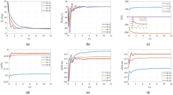
Figure 8.
Simulation results of case 2 with variable N, where (a,b) denote the response curves of the states, (c) denotes the four constraint satisfaction cases, and (d–f) denote the response curves of the inputs.
The state variables and are both stabilized at about 9 s and reach the desired position. Figure 8c shows that both and satisfy the constraints. The UAM is not easily stabilized due to the simultaneous consideration of internal and external disturbances. The tilt angle reaches the desired position more slowly for N = 5. The lateral thrust of the propeller and the torque of the two wheels are compensated with inputs of 0.2 N, 0.5 N·m, and 0.6 N·m. For N = 8, an oscillation occurs, although the tilt angle reaches the desired position quickly. The oscillation of the angular velocity is even larger, reaching a maximum of 50 deg/s, which cannot be used as the optimal prediction interval length.
By balancing the adjustment time and the overshoot, the prediction interval length is optimally selected as .
4.2.2. Selection of Optimal Sampling Period
In order to optimize the sampling period , the value of is initially selected as 0.02 s, 0.03 s, 0.04 s, and 0.05 s. The simulation results are shown in Figure 9, where N = 7 and . The computational time is 388 s, 332 s, 286 s, 216 s, respectively.
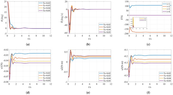
Figure 9.
Simulation results of case 2 with variable , where (a,b) denote the response curves of the states, (c) denotes the four constraint satisfaction cases, and (d–f) denote the response curves of the inputs.
In Figure 9, the state variable is kept in the range of 0°∼26°. The control input is in the range of ∼, while the control inputs and are in the range of ∼. The constraints in Section 3.2 are met. Although the disturbances on the UAM system are large, the desired values are derived at about 8 s, where the disturbances include the UAM physical parameter uncertainty, the white noise and the wind disturbance. This is due to the fact that the system inputs , , are all compensated accordingly.
In Figure 9a,b, the state variables and have the shortest regulation time when . In addition, the state curves are smoother with fewer oscillations when . The state fluctuates at a maximum of 40 deg/s when . However, the curves fluctuate at a maximum of 60 deg/s with the other three values of . Furthermore, the compensation of inputs is also the least when . As can be seen in Figure 9d–f, the compensations are, respectively, 0.026 N, 0.2 N·m, 0.18 N·m. Therefore, the sampling period is optimally selected as .
4.2.3. Different Initial Tilt Angle
The initial tilt angle is chosen as , with the optimal prediction interval length N = 7 and the optimal sampling period = 0.02 s. The obtained prediction results are shown in Figure 10. The computational time is 266 s, 284 s, 223 s, 235 s, respectively.
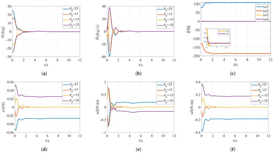
Figure 10.
Simulation results of case 2 with variable , where (a,b) denote the response curves of the states, (c) denotes the four constraint satisfaction cases, and (d–f) denote the response curves of the inputs.
The UAM system can be stabilized at about 7 s even if the initial angle is large. This is due to the fact that both N and are optimal parameters. The state is always in the range of −25°∼25°. The control input is in the range of ∼0.06 . The control inputs and are in the range of ∼1 . Furthermore, the constraints in Section 3.2 are satisfied.
Figure 10 shows that the stable velocity with a large is slower than that with a small . This is because a large needs a great propeller lateral thrust and large wheel torques. When , the propeller lateral thrust is compensated by N. The two wheel torques are both compensated by about . This is because the system is subject to both external and internal disturbances, and it is difficult to reach the desired state.
All curves in Figure 10 oscillate when the wind force reaches its maximum at 4.5 s. However, the curves stabilize after 6 s. Therefore, the developed controller can respond to the disturbance in time. The control effect is better regardless of the initial tilt angle.
In Figure 10, the tilt angles approach deg. The tilt angular velocities, respectively, approach deg/s, deg/s, deg/s and deg/s with initial tilt angles of 25 deg, 15 deg, −15 deg and −25 deg. The values of , respectively, approach 107.73, −186.34, −0.66 and −0.66. The values of input , respectively, approach N, N, N and N with initial tilt angles of 25 deg, 15 deg, −15 deg and −25 deg. The values of input , respectively, approach N · m, N · m, N · m and N · m with initial tilt angles of 25 deg, 15 deg, −15 deg and −25 deg. The values of input , respectively, approach N · m, N · m, N · m and N · m with initial tilt angles of 25 deg, 15 deg, −15 deg and −25 deg. Compared with case 1, the system adjustment time becomes slightly longer in this case. This is because of considering the UAM quality uncertainty and the white noise disturbance. However, the curves in Figure 10 tend to be stable at about 8 s. Therefore, the designed controller can comprehensively consider the input energy consumption and the realization of stability, and has a certain degree of anti-interference.
5. Discussion
The simulation results in Section 4 show that the proposed NMPC method can effectively control the UAM system under external and internal disturbance. However, the following problems should be solved during real-word physical experiments.
- (1)
- Actuator saturation. During physical experiments, the UAM motors have characteristics of limited torque and limited thrust. This easily leads to the problem of actuator saturation. The problem becomes serious under internal and external disturbances. Hence, the stability of the control system cannot be guaranteed. For future study, the anti-windup strategy and the optimization of torque allocation will be considered.
- (2)
- Sensor noise. The sensor noise leads to the accuracy of parameter measurements, including the UAM position, the UAM attitude, the UAM linear velocity, the UAM angular velocity, and so on. The low-pass filtering method and the adaptive smoothing method will be considered for future studies.
- (3)
- Real-time computation constraints. The implementation of NMPC on embedded processors should follow the constraint that the calculations are successfully performed within the sampling time, especially in the case with dynamic compensation. The code optimization method will be further studied with high efficiency.
6. Conclusions
An NMPC-based method is proposed for the UAM stabilization on transmission pipelines under wind field disturbance, where a contact mechanism is developed for the pipeline inspection with high accuracy. The model of wind disturbance is established and is integrated into the UAM dynamics. Based on the established UAM dynamics with disturbance factors and the constructed no-slip constraints, the NMPC method is developed for the UAM system. The asymptotic stability of NMPC is guaranteed by designing the terminal domains and terminal penalties. According to the numerical simulation results, the designed control strategy contributes to the stable state of UAM. In addition, it can effectively overcome factors such as model inaccuracy and disturbance in the process of the control system.
Author Contributions
Conceptualization, S.Z., J.Y. and C.C.; methodology, S.Z. and C.C.; software, S.Z. and J.Y.; validation, X.Z. and L.L.; formal analysis, J.Y. and L.L.; investigation, S.Z. and J.Y.; resources, S.Z. and J.Y.; writing—original draft preparation, S.Z. and J.Y.; writing—review and editing, S.Z. and C.C.; visualization, J.Y. and X.Z.; supervision, C.C. and X.Z.; project administration, S.Z. and C.C.; funding acquisition, S.Z. and C.C. All authors have read and agreed to the published version of the manuscript.
Funding
This work was supported by the National Natural Science Foundation of China (No. 62303367, 52572487, 62203345), the Foreign Expert Project of China (No. H20240959), the Key Research and Development Program of Shaanxi (No. 2024GX-ZDCYL-03-06), the Youth Innovation Team of Shaanxi Universities (No. 2023997), the Key Research and Development Program of Shaanxi (No. 2023-ZDLNY-61), and the Young Talent Nurturing Program of Shaanxi Provincial Science and Technology Association (No. 20240109).
Institutional Review Board Statement
Not applicable.
Informed Consent Statement
Not applicable.
Data Availability Statement
The original contributions presented in the study are included in the article, further inquiries can be directed to the corresponding author.
Conflicts of Interest
The authors declare no conflicts of interest.
References
- Godinez-Garrido, G.; Santos-Sánchez, O.J.; Romero-Trejo, H.; García-Pérez, O. Discrete integral optimal controller for quadrotor attitude stabilization: Experimental results. Appl. Sci. 2023, 13, 9293. [Google Scholar] [CrossRef]
- Ryll, M.; Bülthoff, H.H.; Giordano, P.R. A novel overactuated quadrotor unmanned aerial vehicle: Modeling, control, and experimental validation. IEEE Trans. Control Syst. Technol. 2014, 23, 540–556. [Google Scholar] [CrossRef]
- Yan, Y.; Liang, Y.; Zhang, H.; Zhang, W.; Feng, H.; Wang, B.; Liao, Q. A two-stage optimization method for unmanned aerial vehicle inspection of an oil and gas pipeline network. Pet. Sci. 2019, 16, 458–468. [Google Scholar] [CrossRef]
- Dey, P.K. A risk-based model for inspection and maintenance of cross-country petroleum pipeline. J. Qual. Maint. Eng. 2001, 7, 25–43. [Google Scholar] [CrossRef]
- Wasim, M.; Ullah, M.; Iqbal, J. Gain-scheduled proportional integral derivative control of taxi model of unmanned aerial vehicles. Rev. Roum. Sci. Tech-el. 2019, 64, 75–80. [Google Scholar]
- Mo, H.; Farid, G. Nonlinear and adaptive intelligent control techniques for quadrotor UAV—A Survey. Asian J. Control. 2019, 21, 989–1008. [Google Scholar]
- Kotarski, D.; Benic, Z.; Krznar, M. Control design for unmanned aerial vehicles with four rotors. Interdiscip. Descr. Complex Syst. 2016, 14, 236–245. [Google Scholar] [CrossRef]
- Yu, C.; Yang, Y.; Cheng, Y.; Wang, Z.; Shi, M.; Yao, Z. UAV-based pipeline inspection system with swin transformer for the EAST. Fusion Eng. Des. 2022, 184, 113277. [Google Scholar] [CrossRef]
- Tsintotas, K.A.; Bampis, L.; Taitzoglou, A.; Kansizoglou, I.; Gasteratos, A. Safe UAV landing: A low-complexity pipeline for surface conditions recognition. In Proceedings of the IEEE International Conference on Imaging Systems and Techniques, Virtual, 24–26 August 2021; IEEE: Piscataway, NJ, USA, 2021; pp. 1–6. [Google Scholar]
- Zhou, Q.; Li, X. Experimental investigation on climbing robot using rotation-flow adsorption unit. Robot. Auton. Syst. 2018, 105, 112–120. [Google Scholar] [CrossRef]
- Fan, J.; Xu, T.; Fang, Q.; Zhao, J.; Zhu, Y. A novel style design of a permanent-magnetic adsorption mechanism for a wall-climbing robot. J. Mech. Robot. 2020, 12, 035001. [Google Scholar]
- Zhu, H.; Guan, Y.; Wu, W.; Zhang, L.; Zhou, X.; Zhang, H. Autonomous pose detection and alignment of suction modules of a biped wall-climbing robot. IEEE/ASME Trans. Mechatron. 2014, 20, 653–662. [Google Scholar] [CrossRef]
- Bellahcene, Z.; Bouhamida, M.; Denai, M.; Assali, K. Adaptive neural network-based robust H∞ tracking control of a quadrotor UAV under wind disturbances. Int. J. Autom. Control 2021, 15, 28–57. [Google Scholar] [CrossRef]
- Liang, H.; Xu, Y.; Yu, X. ADRC vs. LADRC for quadrotor UAV with wind disturbances. In Proceedings of the 2019 Chinese Control Conference (CCC), Guangzhou, China, 27–30 July 2019; IEEE: Piscataway, NJ, USA, 2019; pp. 8037–8043. [Google Scholar]
- Xing, Z.; Zhang, Y.; Su, C.Y. Active Wind Rejection Control for a Quadrotor UAV Against Unknown Winds. IEEE Trans. Aerosp. Electron. Syst. 2023, 59, 8956–8968. [Google Scholar] [CrossRef]
- Zhang, Y.; Chen, Z.; Zhang, X.; Sun, Q.; Sun, M. A novel control scheme for quadrotor UAV based upon active disturbance rejection control. Aerosp. Sci. Technol. 2018, 79, 601–609. [Google Scholar] [CrossRef]
- Wang, F.; Gao, H.; Wang, K.; Zhou, C.; Hua, C. Disturbance Observer-Based Finite-Time Control Design for a Quadrotor UAV With External Disturbance. IEEE Trans. Aerosp. Electron. Syst. 2020, 57, 834–847. [Google Scholar] [CrossRef]
- Lindqvist, B.; Mansouri, S.S.; Agha-mohammadi, A.A.; Nikolakopoulos, G. Nonlinear MPC for collision avoidance and control of UAVs with dynamic obstacles. IEEE Robot. Autom. Lett. 2020, 5, 6001–6008. [Google Scholar] [CrossRef]
- Li, W.; Ge, Y.; Guan, Z.; Gao, H.; Feng, H. NMPC-based UAV-USV cooperative tracking and landing. J. Frankl. Inst. 2023, 360, 7481–7500. [Google Scholar] [CrossRef]
- Zhang, K.; Shi, Y.; Sheng, H. Robust nonlinear model predictive control based visual servoing of quadrotor UAVs. IEEE/ASME Trans. Mechatron. 2021, 26, 700–708. [Google Scholar] [CrossRef]
- Gulan, M.; Salaj, M.; Rohal’-Ilkiv, B. Tracking Control of Unforced and Forced Equilibrium Positions of the Pendubot System: A Nonlinear MHE and MPC Approach. Actuators 2023, 12, 343. [Google Scholar] [CrossRef]
- Liu, C.; Chen, W.H.; Andrews, J. Tracking control of small-scale helicopters using explicit nonlinear MPC augmented with disturbance observers. Control Eng. Pract. 2012, 20, 258–268. [Google Scholar] [CrossRef]
- Fnadi, M.; Plumet, F.; Benamar, F. Model predictive control based dynamic path tracking of a four-wheel steering mobile robot. In Proceedings of the 2019 IEEE/RSJ International Conference on Intelligent Robots and Systems (IROS), Macau, China, 4–8 November 2019; IEEE: Piscataway, NJ, USA, 2019; pp. 4518–4523. [Google Scholar]
- Gros, S.; Quirynen, R.; Diehl, M. Aircraft control based on fast non-linear MPC & multiple-shooting. In Proceedings of the 2012 IEEE 51st IEEE Conference on Decision and Control (CDC), Maui, HI, USA, 10–13 December 2012; IEEE: Piscataway, NJ, USA, 2012; pp. 1142–1147. [Google Scholar]
- Yang, C.; Cai, X.; Wu, L.; Guo, Z. Addressing Launch and Deployment Uncertainties in UAVs with ESO-Based Attitude Control. Drones 2024, 8, 363. [Google Scholar] [CrossRef]
- Zhao, S.; Ruggiero, F.; Fontanelli, G.A.; Lippiello, V.; Zhu, Z.; Siciliano, B. Nonlinear model predictive control for the stabilization of a wheeled unmanned aerial vehicle on a pipe. IEEE Robot. Autom. Lett. 2019, 4, 4314–4321. [Google Scholar] [CrossRef]
- Wang, B.; Yan, Y.; Xiong, X.; Han, Q.; Li, Z. Attitude Control of Small Fixed- Wing UAV Based on Sliding Mode and Linear Active Disturbance Rejection Control. Drones 2024, 8, 318. [Google Scholar] [CrossRef]
- Geronel, R.; Botez, R.; Bueno, D. Dynamic responses due to the Dryden gust of an autonomous quadrotor UAV carrying a payload. Aeronaut. J. 2023, 127, 116–138. [Google Scholar] [CrossRef]
- Wang, B.; Ali, Z.A.; Wang, D. Controller for UAV to oppose different kinds of wind in the environment. J. Control Sci. Eng. 2020, 2020, 5708970. [Google Scholar] [CrossRef]
- Cui, L.; Zhang, R.; Yang, H.; Zuo, Z. Adaptive super-twisting trajectory tracking control for an unmanned aerial vehicle under gust winds. Aerosp. Sci. Technol. 2021, 115, 106833. [Google Scholar] [CrossRef]
- Baloch, M.H.; Wang, J.; Kaloi, G.S. Stability and nonlinear controller analysis of wind energy conversion system with random wind speed. Int. J. Electr. Power Energy Syst. 2016, 79, 75–83. [Google Scholar] [CrossRef]
- He, T.; Zhu, Z. Model and Dynamic Analysis of a Three-Body Tethered Satellite System in Three Dimensions. Appl. Sci. 2024, 14, 1762. [Google Scholar] [CrossRef]
- Gros, S.; Zanon, M. Data-driven economic NMPC using reinforcement learning. IEEE Trans. Autom. Control 2019, 65, 636–648. [Google Scholar]
- Wolf, I.J.; Marquardt, W. Fast NMPC schemes for regulatory and economic NMPC—A review. J. Process Control 2016, 44, 162–183. [Google Scholar] [CrossRef]
- Ostafew, C.J.; Schoellig, A.P.; Barfoot, T.D. Robust constrained learning-based NMPC enabling reliable mobile robot path tracking. Int. J. Robot. Res. 2016, 35, 1547–1563. [Google Scholar] [CrossRef]
- Morando, A.E.S.; Bozzi, A.; Graffione, S.; Sacile, R.; Zero, E. Optimizing Unmanned Air–Ground Vehicle Maneuvers Using Nonlinear Model Predictive Control and Moving Horizon Estimation. Automation 2024, 5, 324–342. [Google Scholar] [CrossRef]
- Qian, X.; Shen, H.; Yin, Y.; Guo, D. Nonlinear Model Predictive Control for a Dynamic Positioning Ship Based on the Laguerre Function. J. Mar. Sci. Eng. 2024, 12, 294. [Google Scholar] [CrossRef]
- Grne, L.; Pannek, J. Nonlinear Model Predictive Control: Theory and Algorithms; Springer Publishing Company, Incorporated: Berlin/Heidelberg, Germany, 2013. [Google Scholar]
- He, T.; Zhu, Z.; Luo, J. Stable cargo transportation for underactuated partial space elevator with model uncertainties and disturbances. Adv. Space Res. 2024, 73, 1936–1951. [Google Scholar] [CrossRef]
- Sadraey, M.; Colgren, R. Robust nonlinear controller design for a complete UAV mission. In Proceedings of the AIAA Guidance, Navigation, and Control Conference and Exhibit, Francisco, CA, USA, 15–18 August 2005; p. 6687. [Google Scholar]
- Jafari, M.; Xu, H.; Garcia Carrillo, L.R. A neurobiologically-inspired intelligent trajectory tracking control for unmanned aircraft systems with uncertain system dynamics and disturbance. Trans. Inst. Meas. Control 2019, 41, 417–432. [Google Scholar] [CrossRef]
- Zhu, Z.; Zhong, J.; Ding, M.; Wang, M. Trajectory planning and hierarchical sliding-mode control of underactuated space robotic system. Int. J. Robot. Autom. 2020, 35, 436–443. [Google Scholar] [CrossRef]
Disclaimer/Publisher’s Note: The statements, opinions and data contained in all publications are solely those of the individual author(s) and contributor(s) and not of MDPI and/or the editor(s). MDPI and/or the editor(s) disclaim responsibility for any injury to people or property resulting from any ideas, methods, instructions or products referred to in the content. |
© 2025 by the authors. Licensee MDPI, Basel, Switzerland. This article is an open access article distributed under the terms and conditions of the Creative Commons Attribution (CC BY) license (https://creativecommons.org/licenses/by/4.0/).