Vehicle Collision Frequency Prediction Using Traffic Accident and Traffic Volume Data with a Deep Neural Network

Featured Application

The proposed hybrid deep learning framework integrates nationwide traffic accident and traffic volume data to analyze patterns and key factors associated with a high vehicle crash frequency (F_i). By revealing relationships between roadway characteristics, vehicle composition, and traffic conditions, the model provides valuable insights for targeted safety improvements and policy planning. The approach also establishes a foundation for future applications, including comprehensive risk assessment frameworks, scenario-based safety analysis, and intelligent transportation system (ITS) integration.

Abstract

This study proposes a hybrid deep learning framework for predicting vehicle crash frequency (F_i) using nationwide traffic accident and traffic volume data from the United States (2019–2022). Crash frequency is defined as the product of exposure frequency ($N_a$) and crash risk rate ($\lambda$), a structure widely adopted for its ability to separate physical exposure from the crash likelihood. $N_a$ was computed using an extended Safety Performance Function (SPF) that incorporates roadway traffic volume, segment length, number of lanes, and traffic density, while $\lambda$ was estimated using a multilayer perceptron-based deep neural network (DNN) with inputs such as impact speed, road surface condition, and vehicle characteristics. The DNN integrates rectified linear unit (ReLU) activation, batch normalization, dropout layers, and the Huber loss function to capture nonlinearity and over-dispersion beyond the capability of traditional statistical models. Model performance, evaluated through five-fold cross-validation, achieved R² = 0.7482, MAE = 0.1242, and MSE = 0.0485, demonstrating a strong capability to identify high-risk areas. Compared to traditional regression approaches such as Poisson and negative binomial models, which are often constrained by equidispersion assumptions and limited flexibility in capturing nonlinear effects, the proposed framework demonstrated substantially improved predictive accuracy and robustness. Unlike prior studies that loosely combined SPF terms with machine learning, this study explicitly decomposes F_i into $N_a$ and $\lambda$, ensuring interpretability while leveraging DNN flexibility for crash risk estimation. This dual-layer integration provides a unique methodological contribution by jointly achieving interpretability and predictive robustness, validated with a nationwide dataset, and highlights its potential for evidence-based traffic safety assessments and policy development.

1. Introduction

Traffic accidents remain a critical global issue, causing substantial human casualties and economic losses each year. In 2022 alone, traffic accidents in the United States claimed over 40,000 lives, marking an increase from the previous year and underscoring the urgent need for improved traffic safety [1]. As such, the quantitative analysis and prediction of crash frequency play fundamental roles in accident prevention and traffic safety policymaking [2,3]. Reliable prediction models are particularly essential for the early identification of high-risk locations and for guiding infrastructure improvements.

Traditional approaches to crash frequency prediction have employed statistical models such as Poisson regression and negative binomial models [4]. These models offer clear theoretical underpinnings and are relatively easy to interpret; however, they fall short in accounting for nonlinear interactions, over-dispersion, and multicollinearity that characterize traffic crash data [5]. Moreover, their predictive performance deteriorates rapidly as the number of variables increases due to pre-defined structural assumptions.

In response to these limitations, recent studies have explored ensemble machine learning models such as XGBoost for more accurate crash prediction in urban environments [6].

Recently, deep learning techniques have emerged as promising alternatives for traffic crash prediction. Among them, the multilayer perceptron (MLP) architecture has gained attention for its ability to learn complex patterns and high-dimensional interactions. Its application in traffic safety analysis has been expanding steadily [7,8,9]. Beyond crash prediction, recent studies (2023–2025) have explored advanced spatiotemporal deep learning architectures for traffic flow and risk modeling, including residual convolutional networks, fusion-based methods, and graph transformers [10,11,12]. While these approaches achieve strong predictive performance, they generally treat the crash risk as an end-to-end task without explicitly separating exposure and risk. This distinction underscores the novelty of our framework, which integrates an extended SPF for $N_a$ with a DNN for $\lambda$ estimation to combine interpretability with predictive flexibility. Additionally, hybrid models combining machine learning with variable selection techniques have been proposed to predict crash severity or type [13]. These approaches guided the selection of the input features and model architecture in the present study.

Crash frequency (F_i) is often defined as the product of the crash risk rate ($\lambda$) and exposure frequency ($N_a$), a structure widely adopted in the Highway Safety Manual (HSM) by AASHTO and the FHWA. This decomposition improves interpretability by isolating physical exposure to crashes from the risk of occurrence under specific conditions [14,15].

This study leverages nationwide U.S. traffic crash and volume data (2019–2022) to estimate exposure ($N_a$) and crash risk ($\lambda$) separately and then combine them to predict crash frequency (F_i) using a hybrid deep learning framework (Figure 1). Unlike prior studies that either retained purely statistical SPF-based models or applied machine learning in a black-box manner, our approach explicitly decomposes F_i into $N_a$ and $\lambda$. This allows $N_a$ to be grounded in an extended SPF for interpretability, while $\lambda$ is estimated with a DNN to capture nonlinear interactions.

2. Data and Variables

This study analyzed crash frequency (F_i) based on traffic accident case data and traffic volume data from across the United States for the period 2019–2022. The data consist of accident case data and traffic volume data, and by considering variable importance analysis as well as the methods proposed in the Highway Safety Manual (HSM) of the American Association of State Highway and Transportation Officials (AASHTO) and the Federal Highway Administration (FHWA) of the U.S. Department of Transportation, the crash risk rate ($\lambda$) and exposure frequency ($N_a$) were calculated to derive the final crash frequency (F_i).

2.1. Accident Case Data

Accident case data were collected from actual traffic incidents that occurred across the United States, primarily using the Fatality Analysis Reporting System (FARS) database provided by the National Highway Traffic Safety Administration (NHTSA). The FARS dataset includes detailed information such as crash locations, contributing factors, road conditions, and vehicle characteristics, making it highly suitable for traffic accident analysis.

These variables were used as input features for the deep neural network (DNN)-based crash risk rate ($\lambda$) prediction model. Variable importance analysis was performed to select only the most relevant features. The crash risk rate ($\lambda$) quantifies the relative frequency of crashes occurring under specific conditions. In this study, $\lambda$ was estimated by linking accident case variables with corresponding traffic volume data. The data were preprocessed by encoding categorical variables and standardizing continuous variables.

Table 1. Definition and summary of variables in the vehicle collision case dataset.

Variable Name	Data Type	Value Range/Categories	Description
VNUM_LANNAME	Cat.	1–9, others	Number of travel lanes
VSPD_LIMNAME	Cat.	25–65, others	Speed limit
TRAV_SPNAME (m/s)	Cont.	0–45	Actual vehicle travel speed
HARM_EVNAME	Cat.	Motor Vehicle, Tree, Rollover, etc.	Type of harm
VSURCONDNAME	Cat.	Dry, Wet, Snow, Ice, Others	Road surface condition
BODY_TYPNAME	Cat.	Sedan, SUV, Truck, Bus, Others	Vehicle type
IMPACT1NAME	Cat.	1–12 clock directions	Impact position
STATENAME	Cat.	U.S. states	Location
WEEKDAY_NAME	Cat.	Monday–Sunday	Day of the week

summarizes the key variables in the accident case dataset. Notably, the speed limit (VSPD_LIMNAME) was excluded from the DNN model input and used only for calculating $\lambda$ via Δv estimation.

The selection of variables for the $\lambda$ estimation was based on both prior research and empirical analysis. Δv has been reported to be a strong indicator of speeding-related crashes [16]. Vehicle type and road surface condition were emphasized as critical non-linear predictors by Chang [8] and Xu et al. [7]. Temporal and locational factors, such as weekday and state, were included to capture systematic variations in the crash risk, following Abdel-Aty and Radwan [5].

2.2. Traffic Volume Data

To compute exposure frequency ($N_a$), traffic volume data were collected for road segments across all U.S. states from 2019 to 2022. These data include continuous indicators such as annual average daily traffic (AADT), road length, traffic density, number of lanes, and lane width.

These variables quantify the physical and operational characteristics of road segments and serve as key indicators for evaluating potential crash exposure.

Table 2. Definition and summary of variables in the traffic exposure dataset.

Variable Name	Data Type	Value Range/Categories	Description
STATE_CODE	Cat.	U.S. states	Road location
AADT	Cont.	1–1,277,520 vehicles/day	Avg. daily traffic (all vehicles)
AADT_COMBI	Cont.	0–522,800 vehicles/day	Daily traffic of large trucks
AADT_SINGL	Cont.	0–1,045,600 vehicles/day	Daily traffic of single-unit trucks
LANE_WIDTH	Cont.	2.5–6.5 m	Lane width
ROAD_LENGTH	Cont.	9.8–1998.8 m	Road segment length
TRAFFIC_DENSITY	Cont.	0–1392.5 vehicles/day/m/lane	Density per lane

lists the main traffic volume variables and their definitions.

Rather than being used in isolation, these variables were incorporated into an extended Safety Performance Function SPF-based formula [17]. The extended SPF improves upon the conventional exposure estimation method typically based only on AADT and road length by incorporating additional variables such as truck volume, traffic density, and lane width, thereby enabling a more comprehensive and accurate estimation of exposure frequency.

The inclusion of variables for $N_a$ estimation was guided by the Highway Safety Manual [14] and extended SPF frameworks. Truck-specific traffic volumes were highlighted by Khattak et al. [15] as disproportionately contributing to crash exposure. Lane width and traffic density were incorporated following Wali et al. [17] and Ma et al. [18], who demonstrated their explanatory power in capturing roadway heterogeneity and congestion effects.

Continuous variables were preprocessed by removing missing values and outliers, followed by normalization. To reduce scale differences across datasets, weekly averaging was applied to ensure consistency.

2.3. Data Preprocessing

In this study, nationwide accident and traffic volume datasets were integrated and preprocessed for deep neural network (DNN) training. Preprocessing involved several key stages: organizing variables, handling missing values, encoding categorical variables, normalizing continuous variables, and splitting the data into training, validation, and test sets. These steps were critical for ensuring data quality and optimizing both training stability and model performance.

2.3.1. Variable Organization and Handling of Missing Values

First, column names in both the accident and traffic volume datasets were standardized to ensure consistency. Special characters and spacing were removed to avoid key mismatches during code execution.

Missing values were addressed using machine learning-based predictive imputation, which leverages inter-variable correlations to iteratively estimate and refine missing entries. Key variables such as AADT, ROAD_LENGTH, THROUGH_LA (number of lanes), and TRAFFIC_DENSITY are essential for computing exposure frequency ($N_a$). Missing values for these features can significantly degrade predictive performance. To minimize information loss while preserving structural patterns among variables, a machine learning-based imputation method was adopted instead of simple mean or median replacement.

Specifically, the Iterative Imputer was employed with XGBoost Regressor as the predictive estimator, which is known for its robust performance in handling missing values. Specifically, a machine learning-based iterative imputation approach combining the Iterative Imputer with the XGBoost Regressor was employed to conduct precise missing value estimation that accounts for nonlinear inter-variable relationships. This approach improved the accuracy and consistency of imputation compared to traditional statistical methods. As a result, samples with missing values could be retained, thereby improving both model reliability and data utilization.

2.3.2. Categorical Variable Encoding

Categorical variables such as speed limit, road surface condition, collision direction, and vehicle body type were converted using one-hot encoding to make them suitable for DNN input. To address the issue of category sparsity caused by variables with many unique values, only the top 10 most frequent categories were retained per variable, and the rest were grouped into an “Other” category. This category reduction strategy was implemented to reduce sparsity, prevent overfitting, and enhance model generalization.

2.3.3. Continuous Variable Normalization

Scale differences among continuous variables can lead to inefficient weight updates and hinder convergence in neural network training. Therefore, standardization was applied using scikit-learn’s StandardScaler, transforming variables to have a zero mean and unit variance. Target variables included traffic volume, road length, lane width, and traffic density.

This normalization improved training stability, optimized the initial weight distribution, and enhanced optimization performance, ultimately improving the predictive accuracy.

2.3.4. Dataset Splitting

To enhance generalization and prevent overfitting, five-fold cross-validation was used. The dataset was split into five equal parts. In each iteration, one fold served as validation while the remaining four were used for training.

This method offers the following key advantages over single train–test splits:

• Elimination of bias in the model performance estimation and enhancement of the generalization capability;
• Reliable performance estimation, as all data samples were included once in validation;
• Robust evaluation even when outliers or imbalanced data are present.

Performance was evaluated using metrics including MSE, MAE, and R², and fold-to-fold consistency was analyzed to assess model stability. After tuning the neural network structure and hyperparameters, the final model was trained on the full dataset and saved for subsequent analysis

Additionally, variable importance analyses using both Random Forest and XGBoost validated these selections, and the results were consistent with the literature-based rationale. Travel speed, vehicle type, and road surface condition were identified as the most influential predictors for $\lambda$, while AADT, truck volumes, and traffic density were dominant for $N_a$.

3. Theoretical Basis for Crash Frequency Prediction

Crash frequency ($F_i$) refers to the average number of traffic accidents occurring on a specific road segment over a given time period. It serves as a key indicator in traffic safety analysis and policy development. $F_i$ can be quantitatively expressed using the following basic formulation:

$$F_i=N_a\times \lambda ,$$

(1)

In this formulation, $N_a$ (exposure frequency) denotes the number of opportunities for crashes to occur, commonly measured by physical exposure indicators such as AADT, road length, and lane count. $\lambda$ (crash risk rate) is a dimensionless parameter representing the likelihood of a crash occurring under specific conditions. It is calculated based on multiple environmental and driver-related factors, including vehicle speed, surface condition, vehicle type, time of day, and weekday. This multiplicative structure is grounded in the Safety Performance Function (SPF), as introduced in the Highway Safety Manual (HSM) by AASHTO and the Federal Highway Administration (FHWA) [14,15]. The SPF framework separately estimates $N_a$ and $\lambda$ before combining them to predict $F_i$, a methodology widely adopted in both academic research and engineering practice.

Lord and Mannering (2010) emphasized in their review that structurally separating $\lambda$ and $N_a$ offers interpretability advantages, particularly when addressing nonlinearity, over-dispersion, and variable interaction effects [2]. Modeling $\lambda$ and $N_a$ separately allows complex crash factors to be accounted for flexibly and transparently. Miaou (1994) applied this structure within a negative binomial (NB) regression framework for truck crash analysis. In that study, $N_a$ was estimated using AADT and road geometry, while $\lambda$ reflected the truck type and driving conditions, yielding better accuracy and interpretability than the conventional Poisson model [4]. Later studies extended this structure using statistical methods such as empirical Bayes estimation, Markov switching models, and zero-inflated models [2,5].

While retaining the same theoretical structure, this study introduces a deep learning-based approach to address the limitations of traditional statistical models. Traditional Poisson regression assumes equidispersion, where the mean equals the variance, but crash count data typically exhibit over-dispersion [16]. Negative binomial (NB) regression introduces a dispersion parameter to partially address this issue, yet it still relies on a linear–log structure that limits its ability to capture complex nonlinear relationships [7,8]. These limitations, repeatedly documented in traffic safety research [5,16], motivate the adoption of more flexible approaches such as deep neural networks. Accident and traffic volume data were modeled separately to estimate $\lambda$ and $N_a$, respectively. For the $N_a$ estimation, the conventional SPF was extended to incorporate not only AADT but also traffic density, heavy vehicle proportions, lane count, and lane width. The crash risk rate ($\lambda$) was estimated using a multilayer perceptron (MLP)-based deep neural network that learns nonlinear relationships among input variables, including impact speed, vehicle type, and road condition.

This dual-structured approach provides superior interpretability and predictive accuracy compared to single-regression methods [19]. It is also well suited to address the complexity, imbalance, and high dimensionality of real-world traffic data.

4. Deep Learning-Based Crash Risk Rate ($\mathit{\lambda }$) Estimation

4.1. Theoretical Background

The crash risk rate ($\lambda$) represents the probability of a crash occurring under specific road and traffic conditions. It is influenced by multiple factors, including vehicle speed, surface condition, vehicle type, impact direction, and day of the week. Traditional models estimate $\lambda$ using coefficient-based statistical techniques. However, these methods struggle to capture nonlinear relationships and interaction effects among variables [2,4].

Deep neural networks (DNNs) have recently gained traction in traffic crash prediction due to their ability to model high-dimensional input data and deliver strong predictive performance [7,18]. Some studies have also used DNNs to identify crash-prone segments (blackspots) using historical crash records [20]. The multilayer perceptron (MLP) architecture, known for capturing complex patterns in both categorical and continuous data, was adopted in this study to estimate the crash risk rate $\lambda$.

4.2. Input Variables

The DNN-based $\lambda$ prediction model considered a wide range of crash-related factors. Input variables were grouped into two categories: crash dynamics and environmental context.

• Crash-related variables included travel speed (TRAV_SPNAME), collision direction (IMPACT1NAME), crash severity (HARM_EVNAME), and vehicle type (BODY_TYPNAME). These reflect the dynamics of the crash event.
• Environmental factors included the road surface condition (VSURCONDNAME), state location (STATENAME), and day of week (WEEKDAY_NAME). These contextual variables indirectly reflect risk levels and driver behavior.

All variables were derived from actual crash records and represent conditions at the time of each crash. The model leveraged both categorical and temporal features to improve prediction accuracy, in line with prior studies [21]. Categorical variables were one-hot encoded, and infrequent categories were grouped into an “Other” class to reduce dimensionality and prevent sparsity.

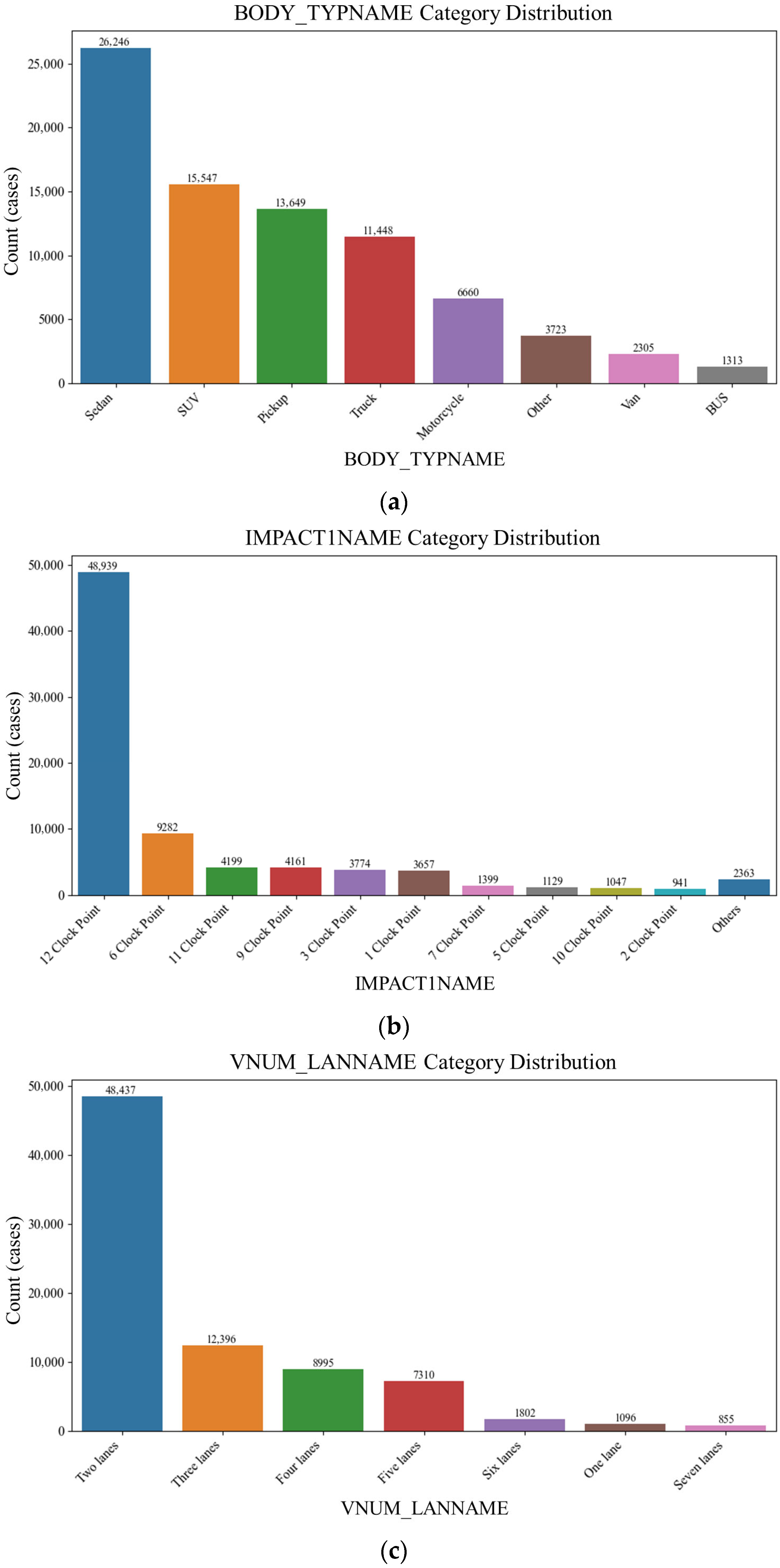
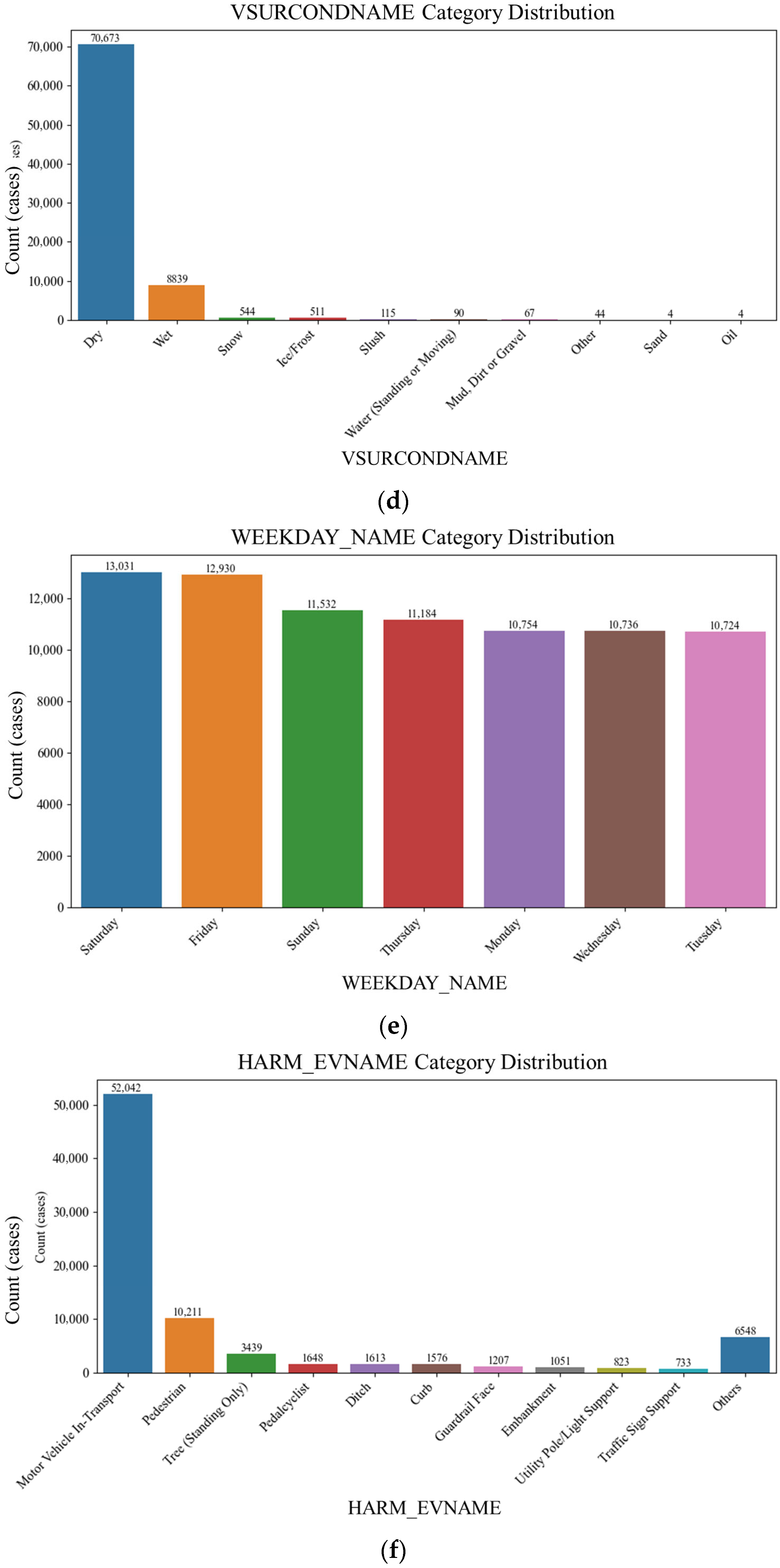
Figure 2 shows the distributions of the categorical input variables used in the crash risk rate estimation. Most categorical variables exhibited a concentration of frequencies in certain categories, indicating data imbalance. For example, passenger cars and SUVs accounted for the majority of vehicle types, and crashes under dry road conditions far outnumbered those under other surface conditions. Such distribution characteristics can cause weight bias during model training; thus, category reduction and balance adjustment were implemented.

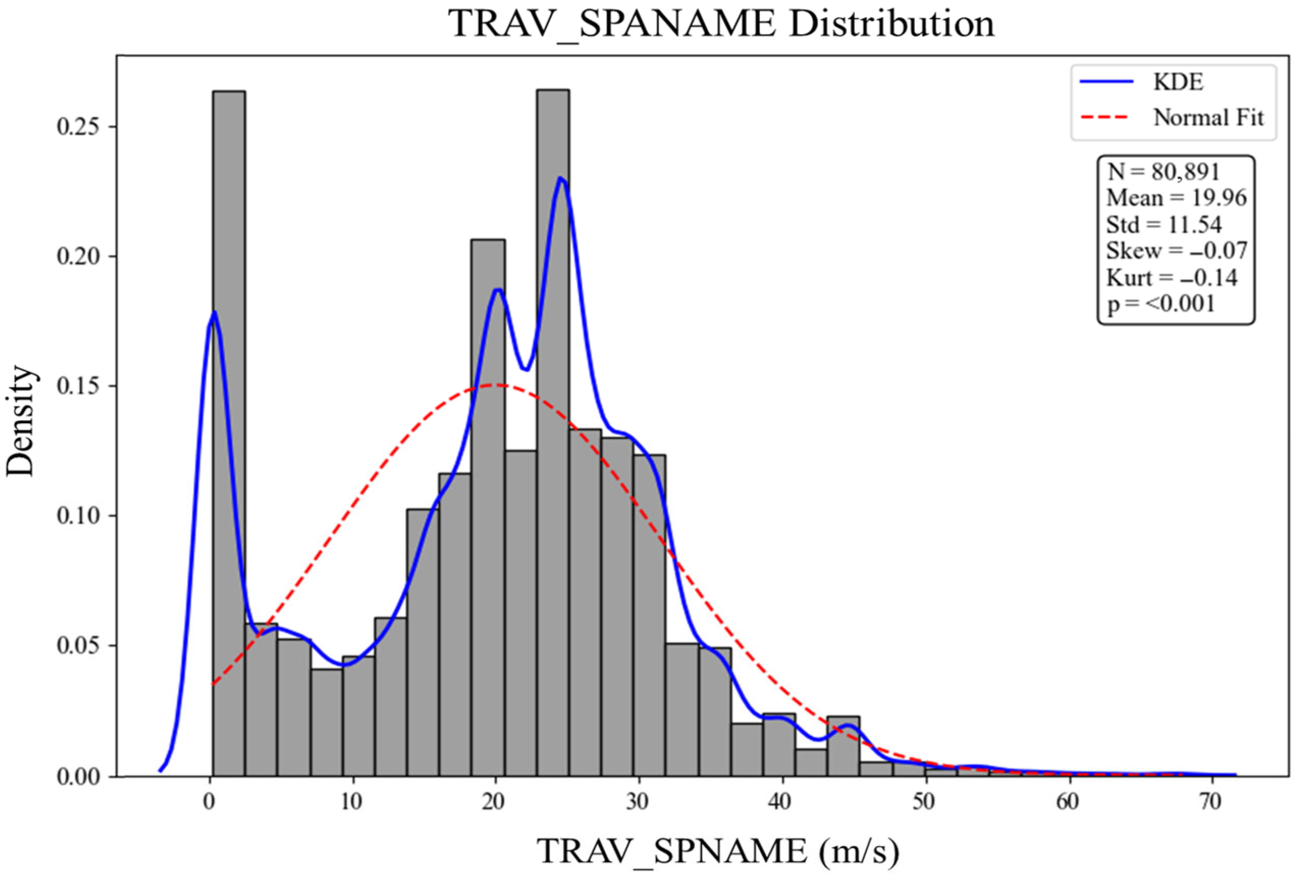
Figure 3 illustrates the distribution of the continuous variable TRAV_SPNAME (vehicle travel speed at the time of collision). Continuous variables such as TRAV_SPNAME were standardized to have a mean of zero and a standard deviation of one using the StandardScaler, which contributed to improving the convergence speed of weights and preventing overshooting in the early stages of training. The figure shows that speeds are concentrated around 25 m/s (approximately 90 km/h), with both the mean and median around 20 m/s, consistent with typical crash characteristics in U.S. urban and highway segments. Outliers above 35 m/s occurred infrequently and were effectively handled through normalization and clipping adjustments.

4.3. DNN Model Structure and Hyperparameters

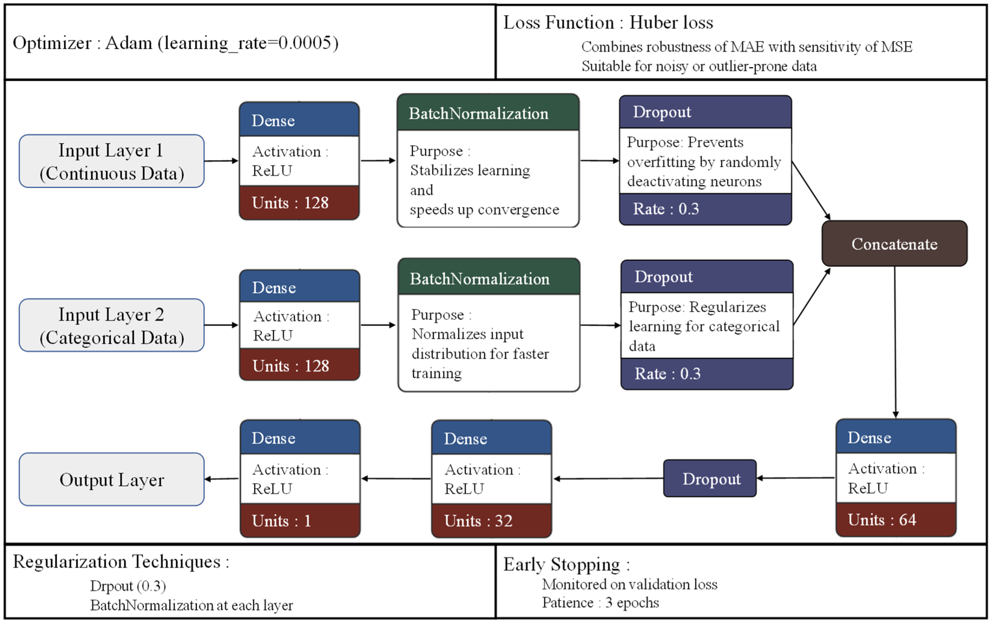
The proposed DNN model employed a hybrid architecture with separate pathways for continuous and categorical inputs, which were later merged for the final prediction. Each input stream continuous and categorical was processed through Dense (128) → Batch Normalization → Dropout (0.3) layers.

The merged features were passed through additional layers (Dense (64) → Dropout (0.3) → Dense (32)) before the final output layer. ReLU activation in the output layer ensured non-negativity and enhanced numerical stability. This dual-pathway architecture captured heterogeneous data structures and improved both prediction accuracy and model generalization [16,18,22].

To estimate crash risk rate ($\lambda$) with high precision, a multilayer perceptron (MLP)-based deep learning structure was adopted. The MLP can effectively learn nonlinear relationships and interaction effects among high-dimensional variables, delivering superior predictive performance compared to conventional linear regression-based approaches [16,18]. Considering the presence of outliers and class imbalance often observed in traffic accident data, the model incorporated batch normalization, dropout, and the Huber loss function to enhance robustness and prediction accuracy. In addition, high $\lambda$ region error analysis and average performance evaluation based on k-fold cross-validation were conducted to further assess model reliability.

4.3.1. Definition of $\lambda$ and the Dependent Variable in the DNN Model

In this study, $\lambda$ was defined as a dimensionless risk rate predicted from crash level variables. Exposure-related factors were modeled separately through $N_a$ to avoid redundancy. The Δv variable (actual speed minus speed limit), based on Kloeden et al. [16], was included to capture speeding behavior a critical indicator of crash risk. This definition provides empirical reliability by capturing the relative relationship between observed crash rates and traffic exposure under varying conditions.

4.3.2. DNN Architecture

The DNN developed in this study follows the structure described below:

• Input layer—processes continuous inputs (2 variables) and categorical inputs (approximately 170 variables after one-hot encoding) using a dual-input structure.
• Hidden layers—

  ‑

  Continuous input pathway—Dense (128) → Batch Normalization → Dropout (0.3)

  ‑

  Categorical input pathway—Dense (128) → Batch Normalization → Dropout (0.3)

  ‑

  Merged pathway—Dense (64) → Dropout (0.3) → Dense (32)

• Activation function—ReLU was applied to all Dense layers.
• Normalization and dropout—Batch normalization and dropout (rate = 0.3) were applied to each input pathway.
• Output layer—ReLU activation (activation = ‘relu’) for positive continuous outputs.

Figure 4 presents the DNN architecture for the crash risk rate prediction.

4.3.3. Hyperparameter Configuration

Model performance was also influenced by hyperparameter settings, which are summarized in

Table 3. Hyperparameter settings and rationale for the deep neural network model.

Parameter	Setting	Rationale
Hidden Layer Structure	[{Dense (128) → BN → Dropout} → Concatenate → Dense (64) → Dropout (0.3) → Dense (32) → Output (1, ReLU)]	Gradual reduction to mitigate overfitting and stabilize learning
Activation Function	ReLU	Standard for nonlinear learning in a DNN
Dropout Rate	0.3	Commonly used value to prevent overfitting [22]
Normalization	Batch Normalization	Enhances training stability and convergence
Loss Function	Huber Loss/MSE	Balances robustness to outliers with accuracy [23]
Optimizer	Adam	Adaptive learning rate, fast convergence
Learning Rate	0.001	Typical initial value with good convergence
Epochs	200	Sufficient training with early stopping
Early Stopping	Patience = 10	Prevents overfitting when validation loss stagnates

.

These settings were based on configurations validated in previous studies. In particular, Huber loss was selected to enhance robustness against outliers in crash risk data [23]. While some models use time-series input to predict crash timing [24], our approach focuses on static features for the risk estimation.

4.4. Model Training and Performance Evaluation

4.4.1. Quantitative Performance

Five-fold cross-validation was conducted to evaluate model performance. Each fold used 20% of the data for validation and 80% for training. Metrics included MSE, MAE, and R², with average values of 0.0485, 0.1242, and 0.7482, respectively.

The results indicated strong explanatory power and low prediction error across varying road and crash scenarios. Figure 5 shows that the predicted and actual values were closely aligned around the y = x diagonal, demonstrating robust predictive accuracy. For high-risk thresholding, high-risk segments are defined as those with a crash risk rate λ in the top q-quantile (e.g., q = 0.90). Unless stated otherwise, all high-risk counts, which are highlighted in the figures, and subset error summaries use this quantile-based threshold. This range included a total of 4636 samples, with an average actual value of 2.096 and an average predicted value of 1.7326.

4.4.2. Post Hoc Interpretability Analysis

In addition to predictive performance, model interpretability is crucial for linking outputs to actionable policy implications.

To this end, we applied SHAP (SHapley Additive exPlanations) analysis to the trained DNN to quantify the contribution of each input variable to the crash risk ($\lambda$) prediction.

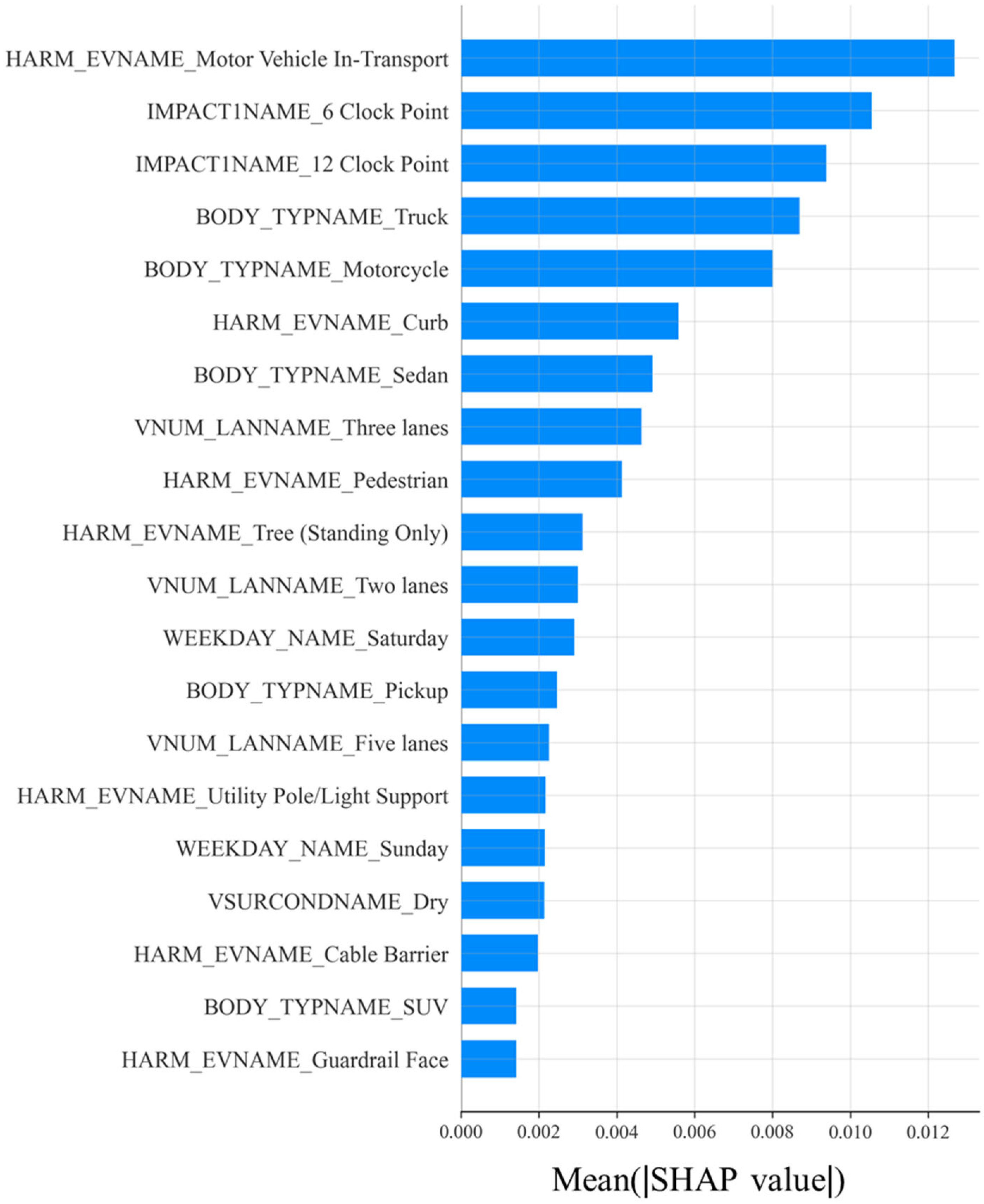
Figure 6 presents the SHAP global feature importance, highlighting travel speed (Δv), vehicle type, and road surface condition as the most influential predictors.

These findings emphasize the critical roles of speeding, vehicle fleet composition, and roadway condition management in traffic safety analysis.

Figure 7 illustrates the distribution of SHAP values for categorical predictors, showing that truck involvement, motorcycles, and specific impact points consistently elevate crash risk contributions, thereby validating the model’s ability to capture heterogeneous crash patterns.

Finally, Figure 8 provides a dependence plot for Δv, where the monotonic upward trend confirms that higher travel speeds substantially increase crash risk contributions.

This outcome aligns with the established traffic safety literature and underscores speeding as a key risk factor.

Taken together, these post hoc interpretability results demonstrate that the proposed framework not only achieves robust predictive accuracy but also yields transparent and explainable insights.

Such interpretability strengthens its relevance for evidence-based policymaking, particularly in the areas of speed management, freight corridor safety, and roadway maintenance strategies.

5. Exposure Frequency (${\mathit{N}}_{\mathit{a}}$) Estimation Method

5.1. Data Composition and Key Variables

Exposure frequency ($N_a$) refers to the total physical opportunities for crashes to occur on a given road segment. It is typically associated with road traffic characteristics such as annual average daily traffic (AADT), segment length, and the number of lanes. In this study, $N_a$ was quantitatively estimated using traffic volume data collected from 2019 to 2022 across various road types in the United States.

The input variables used included AADT, road length (ROAD_LENGTH), lane width (LANE_WIDTH), traffic density (TRAFFIC_DENSITY), combination truck traffic volume (AADT_COMBI), and single-unit truck traffic volume (AADT_SINGL), which are consistent with the exposure factor variables presented in the Highway Safety Manual (HSM) and the related literature [14,15]. In particular, this study incorporated traffic density as an additional variable to more accurately reflect actual traffic flow characteristics, in addition to the AADT values presented in the SPF, by considering vehicle type classifications and roadway congestion.

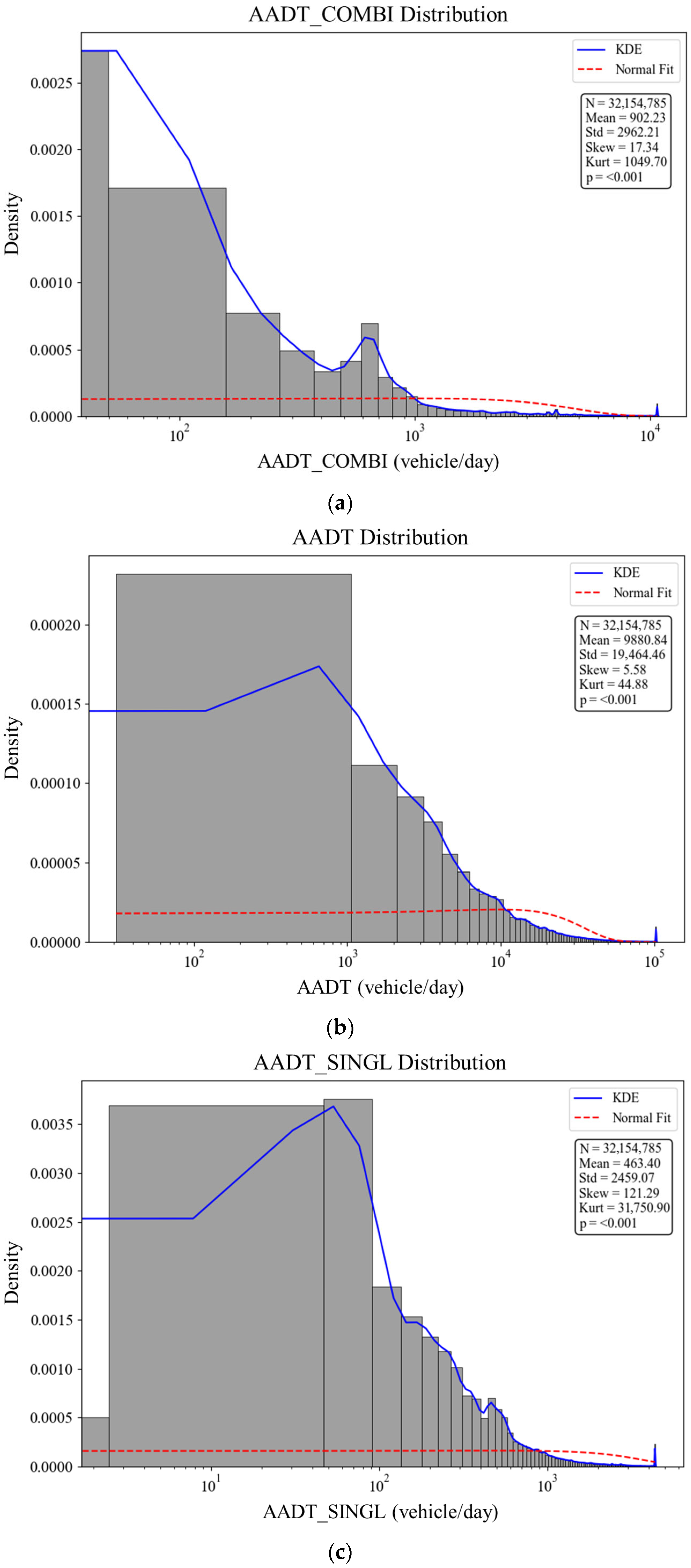
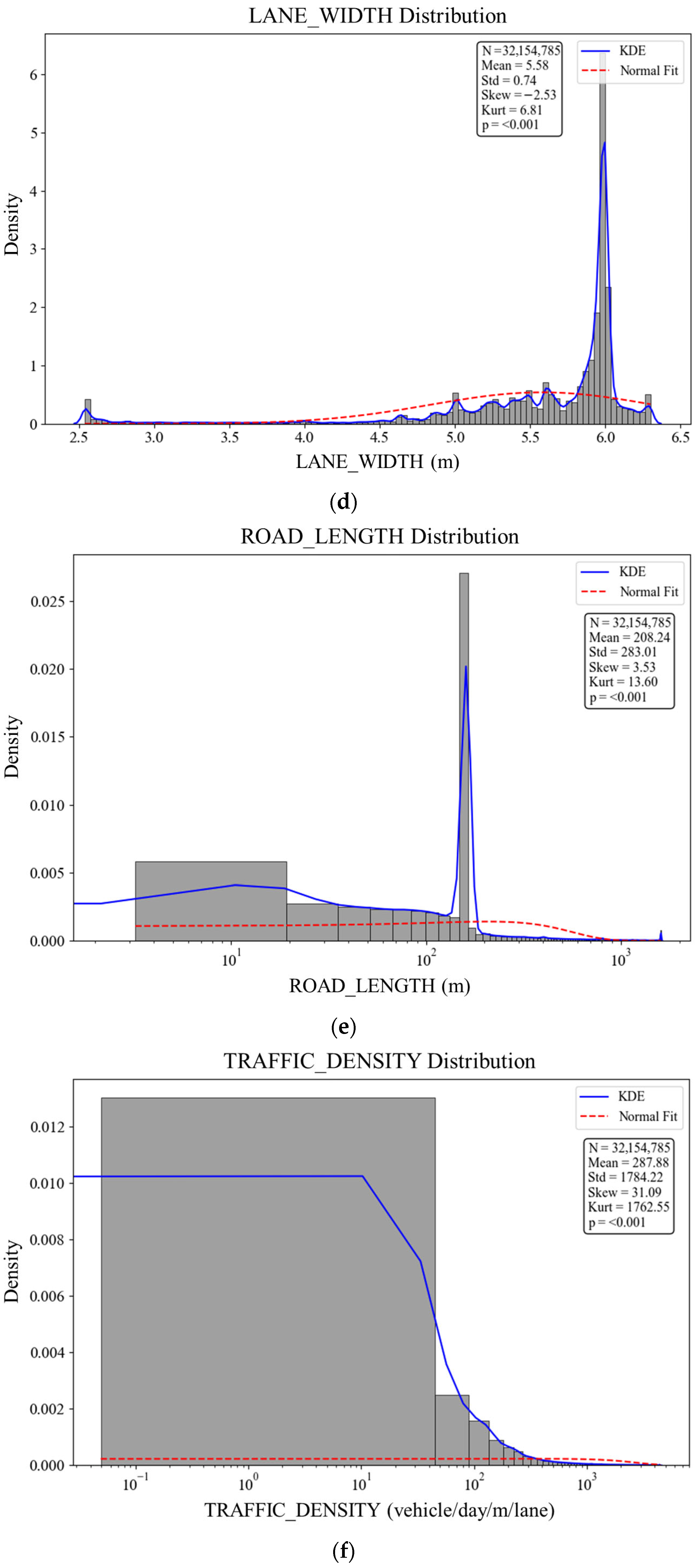
Figure 9 illustrates the distributions of the continuous input variables used in the $N_a$ estimation. Some variables (e.g., AADT, TRAFFIC_DENSITY) displayed patterns similar to a normal distribution, whereas others exhibited extreme skewness, indicating the need for normalization and outlier treatment.

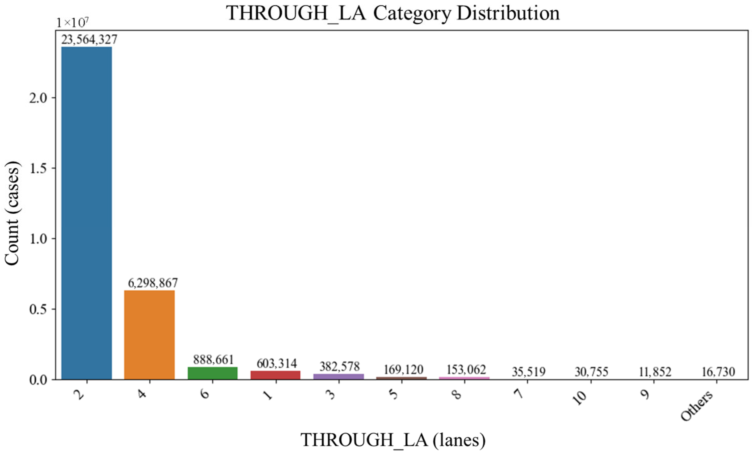
Figure 10 shows the categorical distribution of the number of lanes at the time of the crash. The majority of crashes occurred on two-lane and four-lane roads, with other lane counts showing relatively lower frequencies. Such an imbalance in distribution can cause weight bias in the deep learning model toward certain lane counts. Therefore, rare categories were grouped under an “Other” class to reduce this bias.

5.2. Safety Performance Function (SPF) Theory

The conventional theoretical framework for predicting crash frequency is the Safety Performance Function (SPF), which is conceptually based on estimating crash frequency ($F_i$) as the product of crash risk rate ($\lambda$) and exposure frequency ($N_a$) [2,14]. In particular, the SPF often employs a log–linear regression equation based on the annual average daily traffic (AADT) and has been recognized as an appropriate method for quantifying the actual traffic volume and exposure levels.

The conventional SPF is formulated as follows:

$$N_a=\left({\displaystyle \frac{{AADT}_i \times {Road Length}_i \times {Lane Width}_i}{1000}}\right)\times \left(1+{Traffic Density}_i\right)\times \left(1+0.1·{Truck Ratio}_i\right),$$

(2)

Here,

• Truck Ratio = $\left({\displaystyle \frac{AADT\_COMBI}{AADT\_COMBI+AADT\_SIGL}}\right)$;
• Traffic density, lane width, and road length are considered together to estimate actual exposure in a multidimensional manner;
• A scaling coefficient of dividing by 1000 is included for unit conversion.

This equation is based on the enhanced exposure model proposed by Khattak et al., (2024) [15] and Wali et al., (2018) [17], and it can more flexibly account for complex roadway conditions compared with the simple AADT-based method in the HSM. In particular, by considering dispersion across various roadway types. such as urban/non-urban and highway/non-highway segments. it offers higher explanatory power than conventional regression-based SPFs [18].

This study extends the SPF framework using an AASHTO-inspired model [14,15,17]:

$$N_a=a·{\left(AADT+1\right)}^b·{\left(R_{length}+1\right)}^c·{\left(AAD{T}_C+1\right)}^d·{\left(AAD{T}_S+1\right)}^e·{\left(T_{density}+1\right)}^f·\exp [{\beta }_1·\left(Throug{h}_{La}+1\right)+{\beta }_2·\left(L\_Width+1\right)]$$

(3)

Here, $AADT$ denotes the annual average daily traffic; $R_{length}$ represents the road segment length; $AAD{T}_C$ and $AAD{T}_S$ refer to the traffic volumes of combination and single-unit heavy vehicles, respectively; $T_{density}$ indicates traffic density per unit segment; $Throug{h}_{La}$ is the number of lanes; and $L\_Width$ denotes lane width. This formula enables a more realistic and precise exposure estimation by incorporating the truck composition, traffic density, and roadway geometry in addition to the AADT and road length used in the traditional SPF structure. This approach has been validated for both interpretability and performance through comparisons of various regression- and deep learning-based models on rural highway segments [25].

The coefficients a~f and β₁, β₂ were determined based on previous studies (Khattak et al., 2024; Wali et al., 2018) [15,17] and through the experimental calibration process conducted in this study.

5.3. Exposure Frequency Calculation Results

$N_a$ was calculated independently for each accident case based on the extended formula described above and implemented using parallel computation in the Python-based algorithm (ver.3.10) developed for this study. The calculated $N_a$ values were subsequently combined with $\lambda$ to determine the final crash frequency ($F_i$).

The results showed that $N_a$ values were high on major arterial segments with both a high AADT and long road lengths, and relatively high exposure frequencies were observed in industrial areas and logistics corridors with a high proportion of heavy vehicles. This trend was consistent with the results reported by Khattak et al. (2024) [15] for truck traffic exposure models. In addition, in some urban segments with high congestion (high traffic density), $N_a$ values were higher relative to AADT, confirming that congestion and vehicle composition significantly influence exposure in addition to the simple traffic volume.

This quantitative estimation of exposure frequency serves as the foundation for the crash risk rate ($\lambda$) prediction and final crash frequency ($F_i$) calculation in the following sections and provides an objective basis for identifying road segments with a high actual risk exposure for policy development.

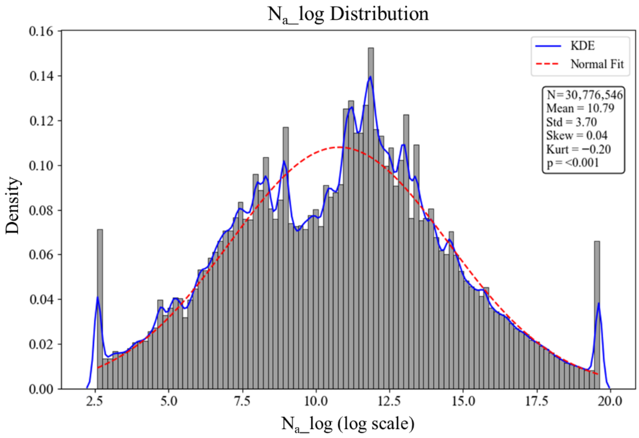
Figure 11 displays the log-transformed distribution of $N_a$, along with the kernel density estimation (KDE) and a fitted normal curve. Both the kernel density estimation (KDE) curve and the fitted normal distribution line are shown, enabling an intuitive assessment of the overall distribution characteristics of $N_a$ and its normality. The distribution exhibits a right-skewed asymmetry, indicating the existence of high-traffic and high-exposure segments. These extreme values are interpreted as originating from traffic-intensive areas such as freight hubs or major interstate corridors, and may act as factors that cause prediction errors during model training.

Accordingly, a log transformation was applied to stabilize the distribution of $N_a$. Since exposure frequency is essentially derived from the product of AADT, road length, and heavy vehicle ratio, it possesses structural characteristics of nonlinear interactions among variables and a power-law form. Directly using such exponential distributions in model training can lead to excessive influence from high values or distortion of weight updates. Log transformation effectively compresses the scale of these power-law-based variables and brings the distribution closer to normality, thereby improving both training stability and interpretability.

The log transformation improved normality, reduced scale disparities, and enhanced model stability. However, in some experiments, it was used only as a normalization factor for training stabilization, while the structural design of the crash risk rate prediction model was configured independently of exposure frequency.

6. Crash Frequency (${\mathit{F}}_{\mathit{i}}$) Prediction and Result Analysis

6.1. Overview of the $F_i$ Calculation Procedure

Crash frequency ($F_i$) was computed as the product of the crash risk rate ($\lambda$) and exposure frequency ($N_a$), a formulation widely recognized in traffic crash modeling. For each crash case, $\lambda$ and $N_a$ were calculated independently and then multiplied. The exposure frequency ($N_a$) was derived using the extended SPF method detailed in Section 5. The crash risk rate ($\lambda$) was predicted using a deep neural network (DNN), based on variables such as travel speed, collision type, road condition, and vehicle classification. The resulting $F_i$ metric captures both the probability and exposure to crashes in specific roadway environments, enabling a more refined risk analysis and targeted safety interventions.

6.2. Predicted Value Distribution and Visualization

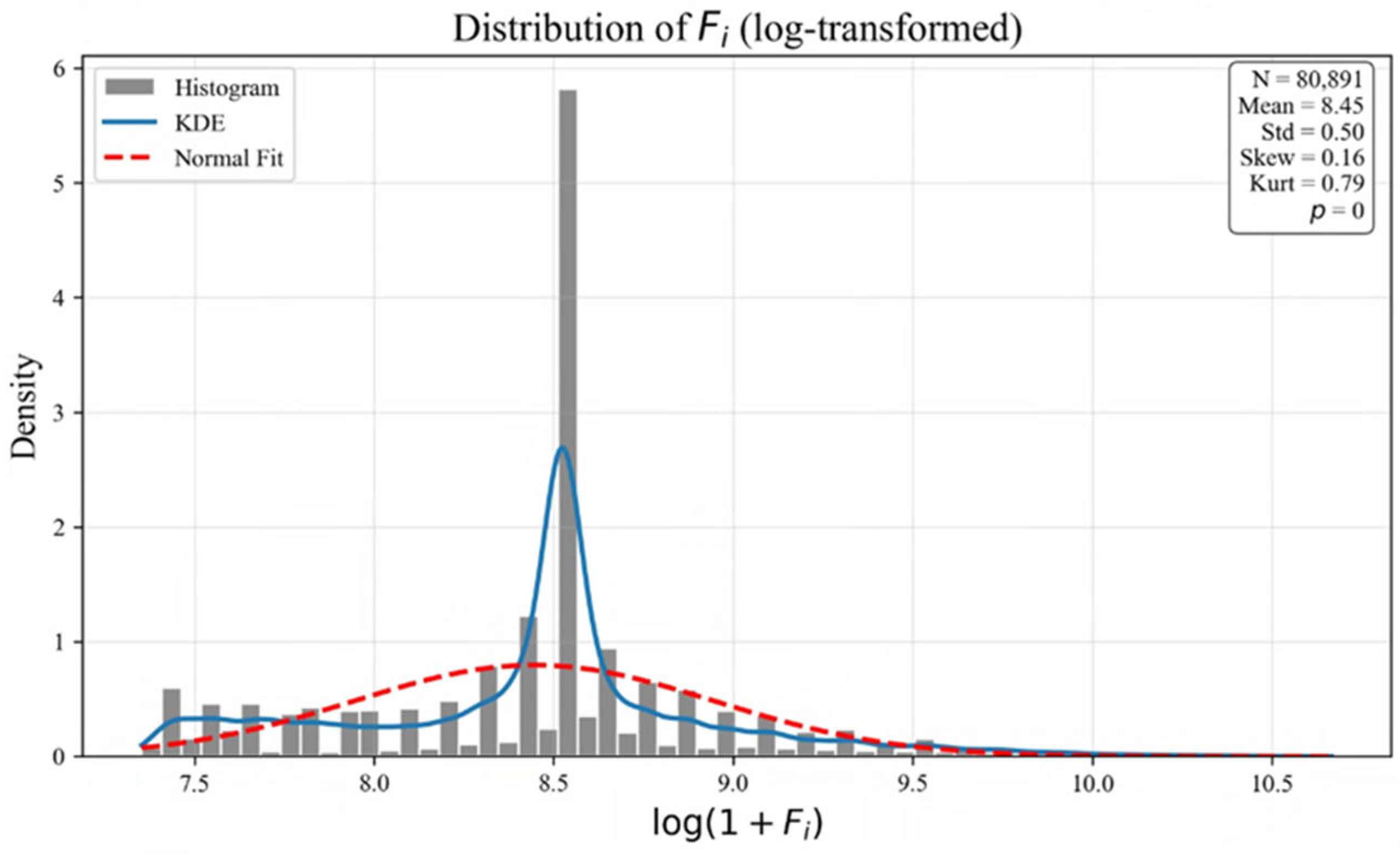
The predicted $F_i$ values displayed a right-skewed, long-tailed distribution, highlighting segments with disproportionately high crash frequencies, particularly in high-traffic and high-risk zones.

Spatial analysis identified key high-risk categories:

• Urban congested areas—$F_i$ was elevated where AADT and traffic density were both high;
• Logistics and industrial corridors—a high proportion of heavy vehicles increased both $\lambda$ and $N_a$, amplifying $F_i$;
• Major highway interchanges—multilane arterials with heavy flow showed peak $F_i$ values;
• Rural segments—typically associated with a low $F_i$ due to minimal exposure and risk.

Dual high-risk areas segments ranking in the top q-quantile for both $\lambda$ and $N_a$ were prioritized for safety interventions. Countermeasures may include infrastructure upgrades, behavioral programs, traffic enforcement, and intelligent transport system (ITS) applications.

Figure 12 shows the distribution of $F_i$ after log transformation. The histogram (gray bars) visualizes the frequency distribution of the dataset, while the kernel density estimation (KDE) curve represents the continuous distribution pattern.

6.3. Prediction Performance Evaluation and Implications

The predicted $F_i$ values were consistent with the segment-level patterns reported in previous studies [15,17], notably in urban congestion zones, freight corridors, and major interchanges. This supports the effectiveness of the proposed hybrid approach, which combines interpretable structure and DNN-based modeling.

Key advantages include the following:

• Structural insights—the separate calculation of $N_a$ and $\lambda$ enables the attribution of the crash risk;
• Accuracy—the DNN model captures complex nonlinearities overlooked in traditional models;
• Policy relevance—the model informs targeted countermeasures based on specific risk contributors.

The $F_i$ predictions thus support practical, evidence-based prioritization of safety improvements tailored to each segment’s risk profile.

7. Conclusions and Future Research Directions

This study integrated nationwide crash case data from the Fatality Analysis Reporting System (FARS) and traffic volume data from 2019 to 2022 in the United States to propose a hybrid crash frequency ($F_i$) prediction framework that combines an extended Safety Performance Function (SPF)-based estimation of exposure frequency ($N_a$) with a deep neural network (DNN)-based prediction of the crash risk rate ($\lambda$).

As discussed in the Introduction, conventional regression-based crash frequency models have inherent limitations in fully capturing nonlinearity, interactions among variables, and issues related to data imbalance. To address these challenges, this study made the following contributions:

• Combining interpretability and predictive power—by separating $N_a$ and λ, the framework ensures both the ability to analyze contributing factors and high predictive precision;
• The DNN model, designed to account for high-dimensional and complex variable structures, demonstrated robust performance (R² = 0.7482);
• Identification of high-risk segments—the framework clearly identified high-$F_i$ segments (e.g., logistics hubs, urban congestion zones, and major highway interchanges).

However, further research is required to produce more reliable results in high-$\lambda$ regions (top-q quantiles, e.g., q = 0.90). Accordingly, the following future improvements are proposed:

• Mitigating data imbalance—applying data augmentation techniques such as SMOTE and GAN for high-risk segments;
• Advancing model architecture—enhancing learning performance through Residual, Attention, and Ensemble structures;
• Integrated risk estimation—combining crash severity indicators to develop a comprehensive risk measure in the form of Risk = F_i × C;
• Assessing real-time applicability—building a real-time crash risk prediction system integrated with intelligent transportation systems (ITSs) and autonomous driving support platforms.

In conclusion, the proposed hybrid prediction framework enables both precise risk predictions and the formulation of cause-specific improvement strategies in road safety analysis. Unlike conventional Poisson and negative binomial regressions, which are often constrained by over-dispersion and restrictive linearity, the framework demonstrated robust predictive performance and produced reliable indicators across diverse conditions. These results highlight its potential as a foundational tool for traffic infrastructure design and operation, policy decision-making, and the future development of intelligent traffic safety management systems. Future work will broaden the scope of benchmarking against additional advanced baselines to further validate robustness across different modeling paradigms.

References

1. National Highway Traffic Safety Administration (NHTSA). U.S. Traffic Deaths Statistics; NHTSA: Washington, DC, USA, 2022. [Google Scholar]
2. Lord, D.; Mannering, F. The statistical analysis of crash-frequency data: A review and assessment of methodological alternatives. Transp. Res. Part A Policy Pract. 2010, 44, 291–305. [Google Scholar] [CrossRef]
3. Washington, S.; Karlaftis, M.; Mannering, F. Statistical and Econometric Methods for Transportation Data Analysis; Chapman and Hall/CRC: Boca Raton, FL, USA, 2010. [Google Scholar]
4. Miaou, S.P. The relationship between truck accidents and geometric design of road sections: Poisson versus negative binomial regressions. Accid. Anal. Prev. 1994, 26, 471–482. [Google Scholar] [CrossRef] [PubMed]
5. Abdel-Aty, M.; Radwan, A.E. Modeling traffic accident occurrence and involvement. Accid. Anal. Prev. 2000, 32, 633–642. [Google Scholar] [CrossRef] [PubMed]
6. Zhang, J.; Wang, Y. Prediction of urban traffic accident risk based on XGBoost algorithm. Appl. Sci. 2022, 12, 298. [Google Scholar] [CrossRef]
7. Xu, C.; Wang, W.; Zhang, M. A deep learning approach for urban traffic accident risk prediction and visualization. PLoS ONE 2020, 15, e0231907. [Google Scholar] [CrossRef]
8. Chang, L.Y. Analysis of freeway accident frequencies: Negative binomial regression versus artificial neural network. Saf. Sci. 2005, 43, 541–557. [Google Scholar] [CrossRef]
9. Kamrani, M.; Arvin, R.; Khattak, A.J. Extracting useful information from connected vehicle data: An empirical study of driving volatility measures and crash frequency at intersections. Accid. Anal. Prev. 2018, 121, 114–122. [Google Scholar] [CrossRef]
10. Zuo, C.; Zhang, X.; Zhao, G.; Yan, L. PCR: A Parallel Convolution Residual Network for Traffic Flow Prediction. IEEE Trans. Intell. Transp. Syst. 2025, 9, 3072–3083. [Google Scholar] [CrossRef]
11. Chen, J.; Pan, S.; Peng, W.; Xu, W. Bilinear Spatiotemporal Fusion Network: An Efficient Approach for Traffic Flow Prediction. Neural Netw. 2025, 187, 107382. [Google Scholar] [CrossRef]
12. Wang, T.; Chen, J.; Lü, J.; Liu, K.; Zhu, A.; Snoussi, H.; Zhang, B. Synchronous Spatiotemporal Graph Transformer: A New Framework for Traffic Data Prediction. IEEE Trans. Neural Netw. Learn. Syst. 2023, 34, 10589–10603. [Google Scholar] [CrossRef]
13. Al Mamun, M.M.; Hossain, S.; Ahmed, F. Traffic accident severity prediction using machine learning algorithms and feature selection techniques. Appl. Sci. 2023, 13, 2455. [Google Scholar] [CrossRef]
14. American Association of State Highway and Transportation Officials (AASHTO). Highway Safety Manual; AASHTO: Washington, DC, USA, 2010. [Google Scholar]
15. Khattak, A.J.; Ahmed, M.M.; Lu, C. Truck traffic exposure and crash risk: Disaggregated AADT impacts by truck type. Sustainability 2024, 16, 1537. [Google Scholar] [CrossRef]
16. Kloeden, C.N.; McLean, A.J.; Moore, V.M.; Ponte, G. Travelling Speed and the Risk of Crash Involvement on Rural Roads; Federal Office of Road Safety: Canberra, Australia, 2001.
17. Wali, B.; Zou, Y.; Ozbay, K. Understanding traffic crash patterns using traffic density and modeling congestion effects. arXiv 2018, arXiv:1803.05074. [Google Scholar]
18. Ma, Y.; Ma, W.; Wang, Y.; Zhang, W.; Huang, H. Modeling crash frequency on urban road segments using a hybrid deep learning framework: A comparative study with traditional statistical and machine learning models. Accid. Anal. Prev. 2023, 195, 107282. [Google Scholar] [CrossRef]
19. Tang, J.; Liang, J.; Han, C.; Li, Z.; Huang, H. Crash injury severity analysis using a two-layer Stacking framework. Accid. Anal. Prev. 2019, 122, 226–238. [Google Scholar] [CrossRef]
20. Zhuang, Z.; Liu, Y. A deep learning-based model for identifying blackspots on highways using historical traffic data. Appl. Sci. 2023, 13, 5296. [Google Scholar] [CrossRef]
21. Bao, J.; Liu, P.; Ukkusuri, S.V. A Spatiotemporal Deep Learning Approach for Citywide Short-Term Crash Risk Prediction with Multi-Source Data. Accid. Anal. Prev. 2019, 122, 239–254. [Google Scholar] [CrossRef]
22. Srivastava, N.; Hinton, G.; Krizhevsky, A.; Sutskever, I.; Salakhutdinov, R. Dropout: A simple way to prevent neural networks from overfitting. J. Mach. Learn. Res. 2014, 15, 1929–1958. [Google Scholar]
23. Huber, P.J. Robust estimation of a location parameter. Ann. Math. Stat. 1964, 35, 73–101. [Google Scholar] [CrossRef]
24. Chen, L.; Zhou, Q.; Lin, Y. Traffic accident forecasting based on time series and deep learning approaches. Appl. Sci. 2022, 12, 3592. [Google Scholar] [CrossRef]
25. Lee, H.; Kim, J. Comparison of machine learning models for crash prediction on rural highways. Appl. Sci. 2021, 11, 1120. [Google Scholar] [CrossRef]
Figure 1. Distributions of the categorical input variables used in the crash risk rate estimation.
Applsci 15 09884 g001
Figure 2. Distributions of categorical input variables used in the crash risk rate estimation: (a) distribution of vehicle body types; (b) distribution of impact locations; (c) distribution of vehicle numbers involved; (d) distribution of surface conditions; (e) distribution of accident weekdays; and (f) distribution of harmful events.
Applsci 15 09884 g002aApplsci 15 09884 g002b
Figure 3. Distribution of the vehicle travel speed at the time of the vehicle collision.
Applsci 15 09884 g003
Figure 4. Deep neural network (DNN) architecture for predicting the risk rate of a crash.
Applsci 15 09884 g004
Figure 5. Comparison of the DNN-based predicted and actual crash risk rates.
Applsci 15 09884 g005
Figure 6. SHAP global feature importance rankings for crash risk predictors.
Applsci 15 09884 g006
Figure 7. SHAP beeswarm plot showing the distribution of categorical variables’ contributions to the crash risk.
Applsci 15 09884 g007
Figure 8. SHAP dependence plot for travel speed.
Applsci 15 09884 g008
Figure 9. Distributions of continuous input variables used in the exposure frequency estimation: (a) distribution of the combined AADT; (b) distribution of the total AADT; (c) distribution of the single AADT; (d) distribution of lane widths; (e) distribution of road lengths; and (f) distribution of traffic density.
Applsci 15 09884 g009aApplsci 15 09884 g009b
Figure 10. Distribution of lane categories used in the exposure frequency estimation.
Applsci 15 09884 g010
Figure 11. Distribution of the log-transformed exposure frequency with the KDE and normal fit.
Applsci 15 09884 g011
Figure 12. Histogram and density of the log-transformed crash frequency.
Applsci 15 09884 g012