Article

The Feasibility of Combining 3D Cine bSSFP and 4D Flow MRI for the Assessment of Local Aortic Pulse Wave Velocity

1
Radiology and Nuclear Medicine, Amsterdam UMC Location University of Amsterdam, Meibergdreef 9, 1105 AZ, Amsterdam, The Netherlands
2
Amsterdam Cardiovascular Sciences, Atherosclerosis and Aortic Disease, Amsterdam UMC Location University of Amsterdam, Meibergdreef 9, 1105 AZ, Amsterdam, The Netherlands
3
Biomedical Engineering and Physics, Amsterdam UMC Location University of Amsterdam, Meibergdreef 9, 1105 AZ, Amsterdam, The Netherlands
*
Author to whom correspondence should be addressed.
Appl. Sci. 2025, 15(18), 10272; https://doi.org/10.3390/app151810272
Submission received: 10 July 2025 / Revised: 11 August 2025 / Accepted: 19 September 2025 / Published: 21 September 2025

Abstract

Pulse wave velocity (PWV) is a key marker of aortic stiffness and cardiovascular risk, yet current methods typically offer only global or regional estimates and lack the possibility to measure local variations along the thoracic aorta. This study aimed to develop and evaluate a pipeline for assessing local aortic PWV using the flow–area (QA) method (PWVQA) by combining high-resolution 4D MRI techniques. A 3D cine balanced steady-state free precession (bSSFP) sequence was used to capture dynamic changes in aortic geometry, while 4D flow MRI measured time-resolved blood flow. The QA method was applied during the reflection-free early systolic phase. Scan–rescan reproducibility was assessed in six healthy volunteers, and feasibility was additionally explored in Marfan syndrome patients. The mean ± SD values of the Pearson correlation coefficients for per-slice maximum area, velocity, flow, and PWVQA were 0.99 ± 0.00, 0.82 ± 0.11, 0.96 ± 0.01, and 0.20 ± 0.35, respectively. The median (Q1–Q3) average PWVQA was 6.6 (5.4–9.4) m/s for scan 1 and 9.1 (6.7–11.3) m/s for scan 2 (p = 0.16) in healthy volunteers and 7.1 (6.9–8.0) m/s in Marfan patients. Combining 4D bSSFP and 4D flow MRI is technically feasible, but the derived PWVQA maps show high variability, particularly in the aortic root and descending aorta, requiring further optimization.

1. Introduction

Altered aortic stiffness can be an important indicator of cardiovascular disease. An adequate elasticity of the aortic wall is needed to create the Windkessel effect, which dampens excessive pressure pulsations in the systemic arteries. Patients with Marfan syndrome are faced with increased aortic wall stiffness and have a heightened risk of aortic dissection and rupture [1]. Moreover, variations in stiffness along the length of the aorta are expected as a result of heterogeneous changes such as elastin disorganization and fragmentation [2]. We hypothesize that areas of increased stiffness may be at higher risk for developing complications, like dissection or rupture. Therefore, assessing aortic wall stiffness locally along its entire length would be highly valuable for the clinical screening and long-term monitoring of conditions like Marfan syndrome.
The direct measurement of arterial stiffness involves assessing vessel diameter and pressure, which requires catheterization—an invasive procedure unsuitable for routine use in healthy volunteers and to a lesser extent in patients [3]. Increased aortic stiffness leads to elevated pulse wave velocity (PWV), causing the earlier arrival of reflected pressure waves in the aorta. This results in increased systolic and pulse pressure, contributing to cardiovascular complications [4]. Noninvasive methods for assessing global PWV using 2D phase-contrast magnetic resonance imaging (PC-MRI) as an indirect measure of arterial stiffness have been introduced for the pulmonary arteries and aorta [3,5,6,7,8,9]. However, the aorta moves down as a result of the mechanical contraction of the heart [10], which creates a through-plane motion that 2D PC-MR acquisitions do not take into account. The 2D PC-MRI-derived global PWV of the ascending aorta may therefore be inaccurate. Moreover, these methods provide a PWV measurement for an entire aortic segment rather than a localized assessment. Four-dimensional PC (4D flow) MRI studies that calculate PWV also overlook aortic motion and typically report PWV over a larger region of the aorta [6,11,12]. While previous work has reported PWV in smaller sub-regions [13], this methodology was still applied to subsections of the static aorta. For accurate and regionally or locally specific PWV measurements, anatomical and 4D flow MRI with high spatial and temporal resolution needs to be used, and the dynamic nature of the aorta needs to be taken into account.
In view of the limitations of current methods to determine local aortic PWV, the aim of this work was to develop a pipeline to assess aortic PWV along the entire length of the thoracic aorta using the flow–area (QA) method (PWVQA). The QA method estimates PWV by calculating the ratio of changes in flow to changes in cross-sectional area during the reflection-free phase of the cardiac cycle in early systole [4,14]. To achieve this, two high-resolution 4D MRI scans were combined: a 3D cine balanced steady-state free precession (bSSFP) sequence capturing dynamic aortic geometry changes and a 4D flow MRI measuring blood flow variations. This study provides a proof of concept for the proposed approach, including scan–rescan reproducibility in six healthy volunteers and additional feasibility testing in six individuals with Marfan syndrome, and reflects on associated challenges and future directions.

2. Materials and Methods

2.1. Acquisition

Six healthy volunteers (self-reported absence of known cardiovascular disease; three women, three men ranging in age from 27 to 45 years) and six Marfan patients (three women, three men ranging in age from 25 to 31 years) underwent cardiovascular magnetic resonance (CMR) on a 3T scanner (Ingenia, Philips, Best, NL, The Netherlands) equipped with a 16-channel dStream Anterior coil and 12-channel posterior coil with Philips smart coil selection. These 12 subjects were chosen from a larger database such that sex was matched. Scans were performed with an in-house developed software modification for accelerated CMR, known as PROspective Undersampling in multiple Dimensions (PROUD) (https://mriresearch.amsterdam/software/aumcproudpatch/, accessed on 21 July 2025) [15]. No contrast agent was administered. The thoracic aorta was imaged under free-breathing using a 3D cine balanced steady-state free precession (4D bSSFP) scan directly followed by a 4D flow scan in the same spatial orientation and angulation and with the same field of view. This protocol was repeated after an interval of 18 ± 17 weeks in the healthy volunteers.
The 4D bSSFP sequence was scanned with repetition time (TR)/echo time (TE)/flip angle (FA) = 2.8–2.89 ms/1.4–1.44 ms/40°; field of view (FOV) FOVFH = 256 mm; FOVAP = 256 or 288 mm; FOVLR = 70 mm or 88 mm; acquired spatial resolution = (1.6 mm)3; reconstructed resolution = (1.0 mm)3; and slice oversampling factor (SOF) = 2.14 for FOVLR = 70 mm or 1.70 for FOVLR = 88 mm with a sinc–Gauss radiofrequency pulse with one sinc period and a mean scan-time of 4 m: 25 ± 7 s. Electrocardiography was used to retrospectively reconstruct data to 30 cardiac phases. Automated self-gating based on repeated k0-lines was used to track respiratory motion throughout the scan. This motion information was then incorporated into a 5D reconstruction, incorporating spatial dimensions, cardiac dynamics, and four respiratory phases. Subsequently, the four respiratory phases were registered and averaged into one expiration phase [16]. The resulting PROUD undersampling factor (R) was Rproud = 19.
The 4D flow scan was conducted with velocity encoding = 150 cm/s; TR/TE/FA = 4.7 ms/2.5 ms/4°; SOF = 1; and a mean scan-time of 7 m:14 s ± 50 s with the same spatial resolution and FOV as those used in 4D bSSFP. Respiratory motion information was acquired using a lung–liver navigator. Retrospective expiratory gating was applied with a minimum window of 5 mm. If the acceptance rate dropped below the set threshold of 55%, this window size was increased in 1 mm increments until the acceptance threshold was met (Supplementary Figure S1). Reconstructing to 60 cardiac phases resulted in a median (Q1–Q3) temporal resolution of 17 (16–19) ms, with a gating window of 6 (5–7) mm, an acceptance rate of 60% (57–62%), and an undersampling factor of Rproud = 27 (26–27).
The local ethics boards approved this study, and written informed consent was obtained from all participants.

2.2. Reconstruction

Both 4D bSSFP and 4D flow compressed sensing reconstructions were performed offline in MATLAB 2021a (The MathWorks Inc. Natick, MA, USA) using MRecon (version 4.4.4., Gyrotools, Zurich, Switzerland) in combination with the Berkeley Advanced Reconstruction Toolbox (BART) [17]. A nonlinear parallel imaging and compressed sensing reconstruction was performed according to
argmin X P F S X Y 2 2 + λ C a r d T V X + λ R e s p T V ( X )
where P denotes the subsampling operator, F the Fourier transform, S the multiplication with sensitivities, Y the raw k-space data, and X the image to be reconstructed. The coil sensitivities S were estimated from the k-space data using the ESPIRiT calibration method available in BART [18]. A sparsifying temporal total variation operator (TV) was applied with for the 4D bSSFP λ C = λ R = 0.1 [16] and for the 4D flow λ C = 0.001 , λ R = 0 [15], both with 20 iterations. For the 4D flow reconstruction, postprocessing was applied including concomitant field correction, 4D Laplacian phase unwrapping [19], and fully automated background phase correction using M-estimate Sample consensus (MSAC) [20]. To match the number of cardiac phases in the 4D bSSFP and the 4D flow scan, the 4D bSSFP images were linearly interpolated to 60 cardiac phases.

2.3. Segmentation, Centerline, and Motion

An nnU-Net trained on 78 manual segmentations from 16 healthy volunteers and 49 Marfan patients was used to automatically segment the thoracic aorta over time from the bSSFP volumes from the root to where the descending aorta leaves the FOV, omitting branching arteries [10,21]. The first cardiac frame, at end-diastole, was used to calculate the reference centerline with the bwskel skeletonization function (Matlab, Mathworks, Natick, MA, USA, version 2021a). The retrieved centerline did not extend all the way to the beginning of the root, requiring some manual input to complete the centerline. The centerline was then smoothed by fitting a spline through the manually defined starting point, the first skeletonized centerline point, and additional points spaced at every 10th of the centerline length. Displacement fields from this first cardiac frame to all subsequent frames were acquired using non-rigid registration based on iterative global deformation using Nc Gaussian radial basis functions with width γ [22,23]. For this study, 30 iterations were used with   N c = 10 k 1   and γ = 1 ( 2   ×   D m e a n ) k 2 where k 1 = k 2 = 2, and Dmean is the mean distance between the source and target meshes. The displacement fields were applied to deform the initial centerline, aligning it with each subsequent phase of the cardiac cycle. To estimate the new tangent direction after transformation, a spline was fitted to the displaced centerline. The tangent to this spline was then calculated and used to determine the updated perpendicular orientations for all planes along the centerline.

2.4. Area and Flow Measurements

Next, area and flow measurements were extracted at each timepoint through a perpendicular plane (width = 53 mm) at each centerline point. The area was calculated by extracting the values of the binary segmentation mask at the x, y, and z coordinates of the perpendicular plane. All non-zero voxels were summed and multiplied by the squared mean voxel size. Since both 4D flow and 4D bSSFP were evaluated in the same FOV and with the same resolution, the aorta segmentation with the centerline was also combined with the velocity data of the 4D flow scan to find the velocity values in each of the three encoding directions per perpendicular plane. This information was then combined to find the through-plane velocity component. The flow was calculated by multiplying the mean velocity through the segmentation by its area for each timeframe. A visual inspection of the velocity profiles through the segmentations in the planes was performed to check that no interscan motion was present that caused misalignment.

2.5. Local PWV Calculation

Finally, a flow–area plot was made for each centerline point, where for each cardiac timepoint, flow was plotted against area, and orthogonal regression was used to estimate the upslope of the flow–area (QA) curve, representing PWVQA [4,14]. The regression points were selected empirically and automatically, starting from the latest timeframe with a flow less than 20% of the maximum flow up to the latest timeframe with a flow less than 80% of the maximum flow. This approach excludes the initial frames before the systolic upslope begins, ensuring that the fitting focuses on early systole—when the assumption of no reflective waves is valid. For this method, at least three fitting points were required to ensure reliable regression. If only two points were available, an additional later timepoint was included. If only one point was available, both an earlier and a later timepoint were added. Given that 3–4 points on the systolic upstroke were used for fitting, and to ensure a balance between goodness of fit and keeping as many PWV values as possible, the fit was considered sufficiently accurate if R2 > 0.85. When necessary, linear interpolation was used to fill in missing values. To enhance local cohesion, a moving mean was applied over five centerline locations. The obtained PWV values were mapped onto the aortic wall. For each plane, the area, average velocity, and flow at their respective peak timeframes, along with PWV, were determined and plotted as a function of location.

2.6. Global PWV Calculation

A global measurement of PWV along the entire aortic length was performed with wave cross-spectrum analysis (PWVWC) [24], making use of the open-source software tool as previously described by Schrauben et al. [25,26] (https://github.com/schrau24/4DFlowPWVTool, accessed on 21 July 2025). For this measurement, the traditional static segmentation based on the phase-contrast magnetic resonance angiogram (PCMRA) was made using an nnU-Net trained on 138 manually segmented 4D flow scans.

2.7. Statistics

The outcomes of this study are the area, velocity, flow, and PWVQA and the correspondence between scan and rescan values. Furthermore, the correspondence between PWVQA and PWVWC is assessed. All continuous parameters are expressed as the mean ± standard deviation unless indicated otherwise. Pearson correlation coefficients were computed to assess the scan–rescan reproducibility of the maximum values across all slices. The average PWVQA was measured as the average over the raw PWV values with R2 > 0.85 only, excluding the interpolated values. The inter-examination differences in average PWVQA were tested with a Wilcoxon signed-rank test, and p < 0.05 was considered statistically significant. The mean difference between repeated measures and limits of agreement (LoA; mean difference ± 1.96 × standard deviation of difference (SDdifference)) and their 95% confidence interval were calculated for Bland–Altman analysis. The Shapiro–Wilk test was used to confirm the assumption of the normality of the difference distributions.
To assess agreement between the global PWVWC measurement method and the averaged local PWV estimate, we constructed two Bland–Altman plots. The first included all scan and rescan measurements from the healthy volunteers, to explore intra-individual variability and evaluate the repeatability of the method. Here the Bland–Altman approach was adapted for repeated measures. For each paired observation, we computed the difference between methods and their average. To account for within-subject correlation due to repeated measurements, we used a one-way analysis of variance (ANOVA) model to partition the total variance of the differences into within-subject and between-subject components. The LoA were then calculated as before but with SDdifference reflecting the combined within- and between-subject variance as recommended by Bland and Altman [27]. Assumptions of normality in the distribution of differences were checked with the Shapiro–Wilk test applied to the mean difference per subject, in order to take into account the effects of intra-subject correlation.
The second plot included the first measurement from each healthy volunteer and the measurements from the Marfan patients, which ensured that the assumption of the independence of observations was upheld.

3. Results

The characteristics of the healthy volunteers and Marfan patients are summarized in Table 1. The Wilcoxon signed-rank test did not show a significant difference in heart rate (p = 0.56), systolic pressure (p = 0.16), and diastolic pressure (p = 0.22) between the repeated measurements in the healthy volunteers.
Figure 1 shows the acquisition and postprocessing pipeline. Panel 1A shows an example bSSFP and 4D flow scan. Panel B contains the segmentations for each cardiac frame after the interpolation of the 3D bSSFP from 30 to 60 cardiac phases. Panel C displays a representative smoothed centerline along with a subset of the calculated perpendicular planes, showing one-fifth of the total for clarity. Figure 1D shows the interpolated area and flow values mapped onto the aortic wall. The values for each centerline point are used to generate the QA plot in panel E, which serves as the basis for calculating the PWV value for each aortic slice. In Supplementary Video S1, a time-resolved version of this figure is presented.
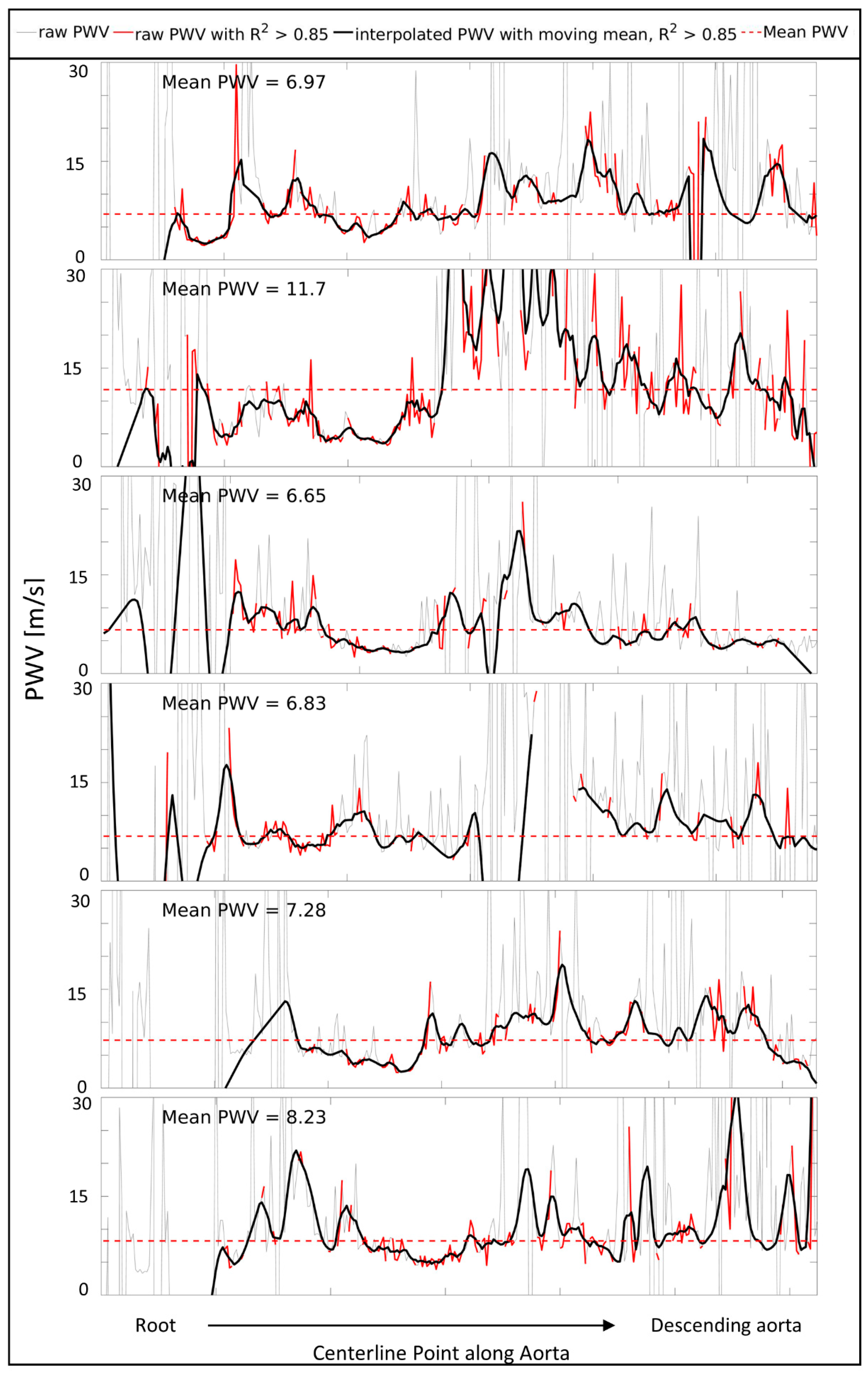
Figure 2 presents the PWV curves along the thoracic aorta for all the first volunteer scans, including the raw measurements, those with R2 > 0.85, and the interpolated, smoothed PWV. Figure A1 in Appendix A contains the same graphs for the six Marfan patients.
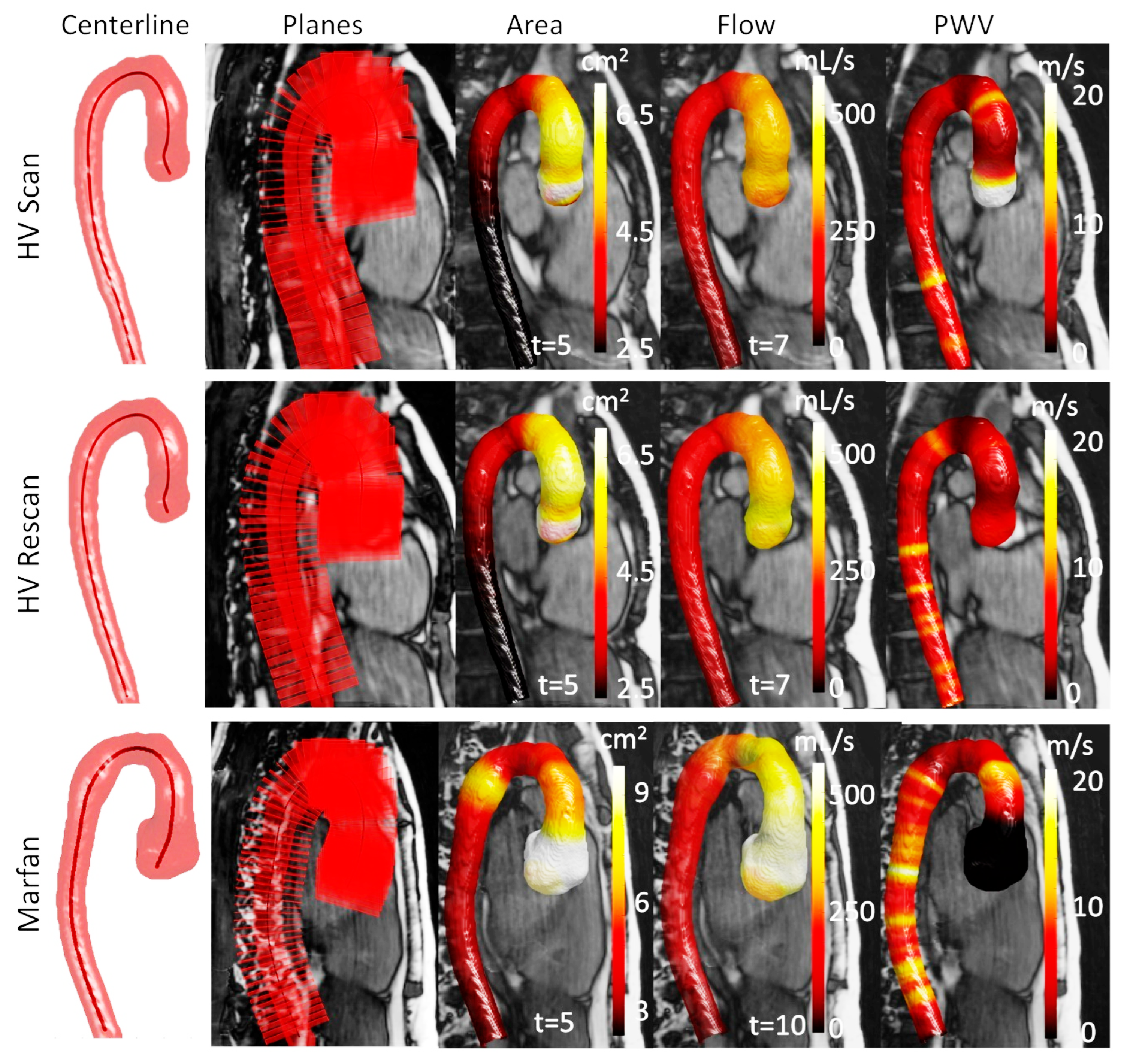
In Figure 3, the segmentations, centerlines, area, flow, and PWV maps of a scan and rescan of one example subject and one Marfan patient are displayed.
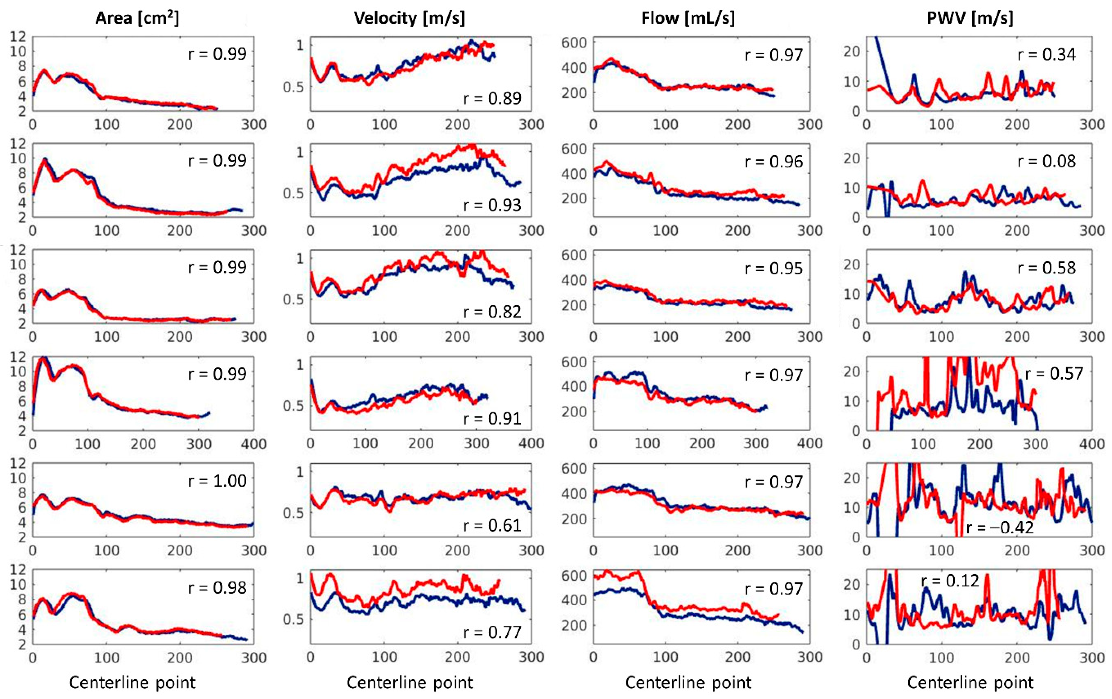
The scan (blue) and rescan (red) results for the maximum area, maximum average velocity, maximum flow, and local PWV per centerline location can be found in Figure 4, in which each row corresponds to one of the six volunteers. The mean ± standard deviation of the Pearson correlation coefficients for area was 0.99 ± 0.00, for velocity 0.82 ± 0.11, for flow 0.96 ± 0.01, and for PWV 0.20 ± 0.35. The median (Q1-Q3) of the average PWVQA for scan was 6.6 (5.4–9.4) m/s and for rescan was 9.1 (6.7–11.3) m/s, and its inter-examination differences were not significant (p = 0.16). The normality of the difference distribution of the data was assessed using the Shapiro–Wilk test, which indicated a significant deviation from normality (p = 0.02). As a result, Bland–Altman analysis was not performed.
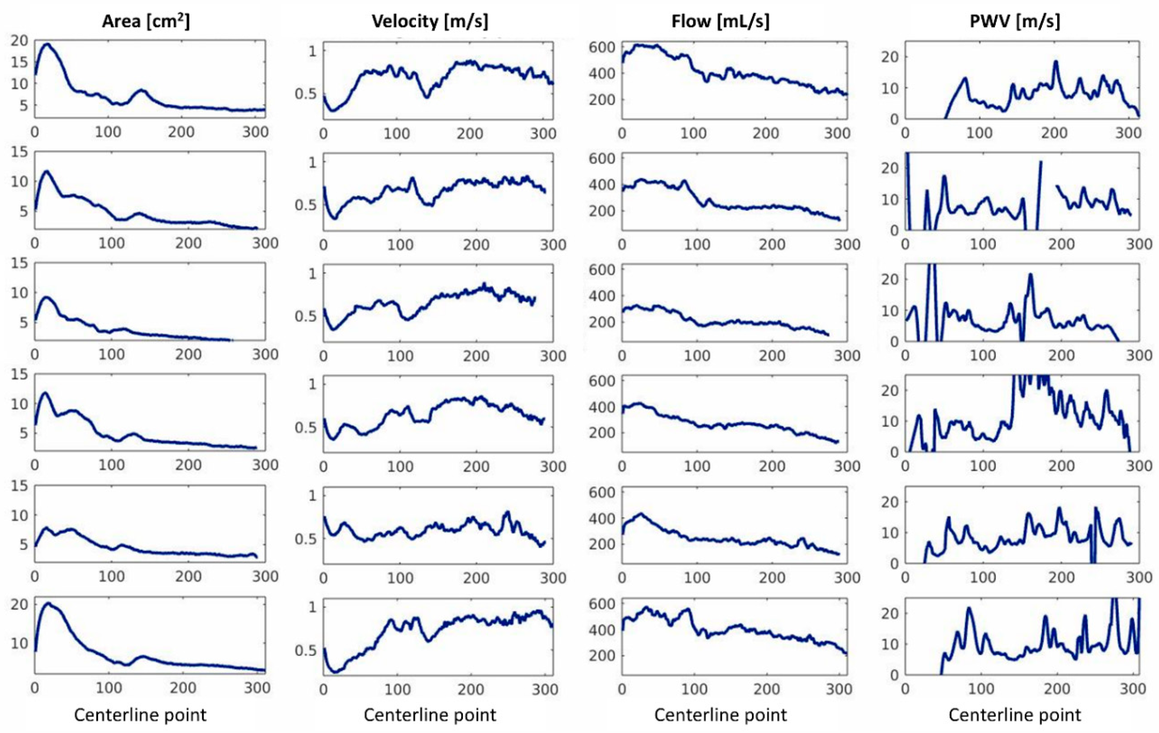
The maximum area, average velocity and flow, and local PWV for the six Marfan patients can be found in Figure 5. Again, each row corresponds to one subject. The median (Q1–Q3) of the average PWVQA for the Marfan patients was 7.1 (6.9–8.0) m/s.
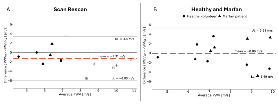
The average PWVQA and global PWVWC for the scan and rescan of each volunteer were determined, and the corresponding Bland–Altman analysis adapted for repeated measures gave a bias ± margin of agreement of −1.31 m/s ± 4.72 m/s and can be found in Figure 6A. Each subject corresponds to a different shape. This plot seems to reveal a trend of increased bias for higher PWV.
Figure 6B combines the first scan of the healthy volunteers with the measurements on the Marfan patients, and Bland–Altman analysis gives a bias ± margin of agreement of −0.09 m/s ± 5.4 m/s.

4. Discussion

In this study, we presented a methodology for the calculation of local pulse wave velocity by the QA method. We found that, despite the good reproducibility for the maximum flow, velocity, and area, the reproducibility for local PWV was low, especially in the aortic root and descending aorta, which seems to indicate that the proposed fitting method is highly sensitive to small errors of velocity and area values. In the descending aorta, minimal area changes and reflective waves may have an effect on the poor reproducibility.
The high cross-correlation coefficient for area confirms the robustness of the automated segmentation pipeline. Repeated velocity measurements reveal that the maximum average velocity can vary between scans, likely due to physiological factors such as heart rate differences. As expected, flow repeatability reflects variations in both area and velocity, as it is a product of the two. However, the PWV measurements derived from the regression of the QA plot upslope show lower correlation coefficients. This suggests that the discrepancies are not due to errors or a lack of reproducibility in the area or flow measurements but rather a loss of quality during the regression step.
Hoskins et al. found typical PWV in the thoracic aorta of about 5 m/s and an increase over the length of the aorta to about 15 m/s in the arteries in the lower leg [28]. Indeed, based on carotid–femoral measures of PWV with tonometry, normal PWV values have been reported as ~6 m/s in young healthy volunteers (<30 years) and up to ~10 m/s in individuals > 70 [6,29]. Other 2D PC-MR-based measures of the aortic arch found a mean value of 3.6 m/s in a cohort of 71 subjects with a mean age of 16.4 ± 7.6 years [30]. PWV measurements for the entire thoracic aorta based on 4D flow MRI have been reported to increase with age from 5.4 m/s in young adults (<45 years) to 7.2 m/s in midlife (45–65 years) and 9.4 in later life (>65 years) [12]. Another study found PWV values of 4.9 m/s in 20–30-year-olds and 8.1 m/s in 70–80-year-olds [11]. In this proof of concept study, the calculated PWVQA plots gave averages within this physiological range, with the local PWV curves in Figure 4 and Figure 5 of three volunteers and two Marfan patients also being largely within these limits of 5–15 m/s.
An analysis of the 2D PWVQA plots revealed particularly high variability in PWV measurements in the aortic root and descending aorta. A possible cause for this increase in variability is the decrease in the amplitude of area change along the descending aorta, which makes the regression of the QA plots potentially more vulnerable to small perturbations. This quality could potentially be improved by further optimizations in the acquisition and postprocessing pipeline that remain to be tested. Although the segmentations and initial centerlines appear identical, an inspection of Supplemental Video S1 reveals small oscillations in the orientation of perpendicular planes, despite the smooth tracking of larger motion. These subtle instabilities may introduce noise, primarily affecting the area measurements. Especially in the regions with small relative area changes, these small changes in orientation can affect the outcome. Moreover, in the root of the ascending aorta, where the shape transitions from the three-cusped annulus to a tubular structure, minor angular deviations could lead to larger area discrepancies, potentially causing the PWVQA method to fail.
Additionally, the high variability in PWVQA measures could perhaps be explained by the relatively small number of timepoints that could be used to fit the systolic upslope of the QA plot. However, exploratory analysis revealed that using 30 cardiac phases did not substantially degrade the quality of the PWV plots compared to the 60 cardiac phases reported here in the healthy volunteers, as shown in Figure A2. In some cases, correlations even showed a slight decrease in variability. This seems to indicate that it is not the number of timepoints but rather data quality which determines fit reliability.
Our strategy of linearly interpolating between locations with a high fit quality of R2 > 0.85 was meant to decrease the impact of failing PWV measures. However, at times, even non-physical, negative, or extremely high pulse wave velocity measures would satisfy this requirement. This causes the occasional extreme peaks visible in Figure 2, Figure 4, and Figure 5 after linear interpolation. Others, like Mura et al., who used cross-correlation between flow curves for the PWV calculation of at most six regions along the thoracic aorta, made an implementation that would simply neglect negative values [13]. While this is a fair assumption, we chose to retain these values to be able to critically evaluate the performance of this method at this moment in time. As shown in Figure 2 and Figure S2, a substantial number of measurements both met and failed to meet the R2 > 0.85 threshold. Possibly, the fit quality might be overestimated using R2 based on a low number of measurements points.

Limitations

A key challenge of the QA method has, in the past, been its long processing time [3,6], primarily due to the need for manual contouring in area determination. Additionally, the manual segmentation of the aortic lumen is often considered subjective and susceptible to inaccuracies [31]. Therefore, one of the great advantages presented in the postprocessing pipeline herein is the automated segmentation of 4D bSSFP scans, which is extremely time-saving while also minimizing interobserver variability. It is important to note that the network was trained on a dataset derived from manual segmentations by two observers, making it inherently subjective and somewhat prone to inaccuracies.
The thresholds of 20% and 80% of the maximum flow were empirically chosen based on Peng et al., who used the linear portion of early systole for regression point determination [32]. While this automated approach ensures consistency, it is also a limitation, as it lacks manual verification or optimization for each QA plot. However, manually selecting regression points for over 200 centerline points per scan is not a practical alternative.
We qualitatively assessed whether bulk motion occurred between 4D bSSFP and 4D flow acquisitions using through-plane velocity images overlaid with segmentation planes. We did not find any motion in this cohort. Future studies in larger cohorts should incorporate the registration of the bSSFP and 4D flow segmentations before the further quantification of PWVQA. Additionally, since the scans were acquired sequentially, heart rate variability could affect temporal resolution, potentially causing a slight misalignment of cardiac bins. Future research could explore reconstructing data with identical temporal resolution rather than an identical number of cardiac bins. This, however, will present its own challenges with larger variability in the undersampling factor per cardiac bin.
Memory limitations influenced the decision to reconstruct 3D bSSFP data into 30 cardiac phases and interpolate it to 60, rather than directly reconstructing all 60 phases. However, since this method primarily relies on early systolic information, restricting reconstruction to systole alone could potentially omit these memory constraints.
Another inherent limitation of the flow–area method is the assumption that measurements are taken during a reflection-free period. Therefore, the QA method should be applied sufficiently high upstream from changes in vascular impedance [7]. The ascending aorta is the most suitable region for applying this method, while the assumption of a reflection-free period may no longer hold by the time the flow wave reaches the descending aorta. The apparent increase in measurement differences observed in Figure 6 for increased mean PWV could potentially be explained by this.
Future work will focus on application in larger cohorts, as the poor reproducibility of local PWV can be reduced by averaging the 3D maps, as has been shown in previous work for wall shear stress [33] such that differences between patient groups and healthy volunteers can be shown at the group level. Also, it would be interesting to evaluate the performance of the local PWV methodology in abdominal aortas, where the effect of cardiac motion will be reduced. However, minimal area change and reflective waves are expected to also have an effect on reproducibility in this region. Both would warrant even higher-resolution 4D bSSFP (spatial resolution) and 4D flow (temporal resolution) MRI to capture these changes. To improve the reproducibility of local PWV in the aortic root, in future work, we aim to segment the aorta with the outflow tract. For the descending aorta, we could experiment with increasing the spatial resolution of the 4D bSSFP to better detect area changes.

5. Conclusions

Combining 4D bSSFP and 4D flow MRI is technically feasible, which was shown in the reproducible slice-wise dynamic aortic area, velocity, and flow maps in six health volunteers and a working pipeline in both healthy volunteers and Marfan patients. However, the derived PWVQA maps show high variability along the aorta, especially in the root and descending aorta, and need further investigation and optimization to become more robust.

Supplementary Materials

The following supporting information can be downloaded at https://www.mdpi.com/article/10.3390/app151810272/s1, Figure S1: Retrospective respiratory gating implementation for the reconstruction of 4D flow images; Video S1: Time-resolved acquisition and postprocessing pipeline; Video S2: Four example planes used for pulse wave velocity calculations.

Author Contributions

Conceptualization, R.M., E.M.S. and P.v.O.; methodology and software: R.M. and E.M.S.; data collection: R.M. and D.B.; data analysis: R.M. and D.B.; interpretation: R.M., E.M.S., G.J.S., A.J.N. and P.v.O.; manuscript preparation: R.M.; manuscript editing and reviewing: R.M., E.M.S., G.J.S., A.J.N. and P.v.O.; supervision: E.M.S., G.J.S., A.J.N. and P.v.O. All authors have read and agreed to the published version of the manuscript.

Funding

This study is part of the research program Applied and Engineering Sciences and the project Comprehensive Assessment of 4D Thoracic Aorta Biomechanics Using Novel Cardiac MRI Technology (number 18402), financed by the Dutch Research Council (NWO).

Institutional Review Board Statement

This study was conducted in accordance with the Declaration of Helsinki and approved by the Institutional Review Board (METC) of Amsterdam UMC (protocol code NL82669.018.22, 5 December 2022). Registered at ClinicalTrials.gov, NCT05944614.

Informed Consent Statement

Informed consent was obtained from all subjects involved in this study.

Data Availability Statement

For this study, we used the Amsterdam UMC ‘PROspective Undersampling in multiple Dimensions’ (PROUD) software patch (https://mriresearch.amsterdam/software/aumcproudpatch/, accessed on 21 July 2025). The individual participant data will not be made publicly available, in accordance with the data sharing plan specified at trial registration on ClinicalTrials.gov. One 4D bSSFP and 4D flow MRI dataset of a healthy volunteer and all code are shared at https://zenodo.org/records/17120266 (accessed on 21 July 2025).

Conflicts of Interest

The authors declare no conflicts of interest. The funders had no role in the design of the study; in the collection, analyses, or interpretation of data; in the writing of the manuscript; or in the decision to publish the results.

Abbreviations

The following abbreviations are used in this manuscript:
bSSFPBalanced steady-state free precession
CMRCardiovascular magnetic resonance
FAFlip angle
FOVField of view
LoALimits of agreement
MRIMagnetic resonance imaging
PCMRAPhase-contrast magnetic resonance angiogram
PC-MRIPhase-contrast magnetic resonance imaging
PROUDProspective undersampling in multiple dimensions
PWVPulse wave velocity
PWVQALocal pulse wave velocity based on flow–area method
PWVWCGlobal pulse wave velocity based on wave cross-spectrum analysis
QAFlow–area
SOFSlice oversampling factor
TEEcho time
TRRepetition time

Appendix A

Figure A1. Pulse wave velocity (PWV) measures starting from the root to the descending aorta for all 6 Marfan patients. Raw PWV (gray), raw PWV with R2 > 0.85 (red), and smoothed, interpolated PWV (black) over the length of the thoracic aorta. The mean PWV based on the red line (raw PWV with R2 > 0.85) is indicated with a red striped horizontal line.
Applsci 15 10272 g0a1
Figure A2. Reproducibility analysis for 30 cardiac timeframes of maximum area, maximum velocity, maximum flow, and pulse wave velocity of all six healthy volunteers.
Applsci 15 10272 g0a2

References

  1. Sonesson, B.; Hansen, F.; Länne, T. Abnormal Mechanical Properties of the Aorta in Marfan’s Syndrome. Eur. J. Vasc. Surg. 1994, 8, 595–601. [Google Scholar] [CrossRef]
  2. Marque, V.; Kieffer, P.; Gayraud, B.; Lartaud-Idjouadiene, I.; Ramirez, F.; Atkinson, J. Aortic Wall Mechanics and Composition in a Transgenic Mouse Model of Marfan Syndrome. Arterioscler. Thromb. Vasc. Biol. 2001, 21, 1184–1189. [Google Scholar] [CrossRef] [PubMed]
  3. Ibrahim, E.S.H.; Shaffer, J.M.; White, R.D. Assessment of pulmonary artery stiffness using velocity-encoding magnetic resonance imaging: Evaluation of techniques. Magn. Reson. Imaging 2011, 29, 966–974. [Google Scholar] [CrossRef] [PubMed]
  4. Vulliémoz, S.; Stergiopulos, N.; Meuli, R. Estimation of local aortic elastic properties with MRI. Magn. Reson. Med. 2002, 47, 649–654. [Google Scholar] [CrossRef]
  5. Metafratzi, Z.M.; Efremidis, S.C.; Skopelitou, A.S.; De Roos, A. The clinical significance of aortic compliance and its assessment with magnetic resonance imaging. J. Cardiovasc. Magn. Reson. 2002, 4, 481–491. [Google Scholar] [CrossRef]
  6. Wentland, A.L.; Grist, T.M.; Wieben, O. Review of MRI-based measurements of pulse wave velocity: A biomarker of arterial stiffness. Cardiovasc. Diagn. Ther. 2014, 4, 193–206. [Google Scholar]
  7. Herold, V.; Parczyk, M.; Mörchel, P.; Ziener, C.H.; Klug, G.; Bauer, W.R.; Rommel, E.; Jakob, P.M. In vivo measurement of local aortic pulse-wave velocity in mice with MR microscopy at 17.6 tesla. Magn. Reson. Med. 2009, 61, 1293–1299. [Google Scholar] [CrossRef]
  8. Shahzad, R.; Shankar, A.; Amier, R.; Nijveldt, R.; Westenberg, J.J.M.; De Roos, A.; Lelieveldt, B.P.F.; Van Der Geest, R.J. Quantification of aortic pulse wave velocity from a population based cohort: A fully automatic method. J. Cardiovasc. Magn. Reson. 2019, 21, 27. [Google Scholar] [CrossRef] [PubMed]
  9. Burris, N.S.; Dyverfeldt, P.; Hope, M.D. Ascending Aortic Stiffness with Bicuspid Aortic Valve is Variable and Not Predicted by Conventional Parameters in Young Patients. J. Heart Valve Dis. 2016, 25, 270–280. [Google Scholar]
  10. Merton, R.; Bosshardt, D.; Strijkers, G.J.; Nederveen, A.J.; Schrauben, E.M.; van Ooij, P. Assessing Aortic Motion with Automated 3D Cine Balanced SSFP MRI Segmentation. J. Cardiovasc. Magn. Reson. 2024, 26, 101089. [Google Scholar] [CrossRef]
  11. Harloff, A.; Mirzaee, H.; Lodemann, T.; Hagenlocher, P.; Wehrum, T.; Stuplich, J.; Hennemuth, A.; Hennig, J.; Grundmann, S.; Vach, W. Determination of aortic stiffness using 4D flow cardiovascular magnetic resonance—A population-based study. J. Cardiovasc. Magn. Reson. 2018, 20, 43. [Google Scholar] [CrossRef]
  12. Jarvis, K.; Scott, M.B.; Soulat, G.; Elbaz, M.S.M.; Barker, A.J.; Carr, J.C.; Markl, M.; Ragin, A. Aortic Pulse Wave Velocity Evaluated by 4D Flow MRI Across the Adult Lifespan. J. Magn. Reson. Imaging 2022, 56, 464–473. [Google Scholar] [CrossRef]
  13. Mura, J.; Sotelo, J.; Mella, H.; Wong, J.; Hussain, T.; Ruijsink, B.; Uribe, S. Non-invasive local pulse wave velocity using 4D-flow MRI. Biomed. Signal Process. Control 2022, 71, 103259. [Google Scholar] [CrossRef]
  14. Rabben, S.I.; Stergiopulos, N.; Hellevik, L.R.; Smiseth, O.A.; Slørdahl, S.; Urheim, S.; Angelsen, B. An ultrasound-based method for determining pulse wave velocity in superficial arteries. J. Biomech. 2004, 37, 1615–1622. [Google Scholar] [CrossRef] [PubMed]
  15. Gottwald, L.M.; Peper, E.S.; Zhang, Q.; Coolen, B.F.; Strijkers, G.J.; Nederveen, A.J.; van Ooij, P. Pseudo-spiral sampling and compressed sensing reconstruction provides flexibility of temporal resolution in accelerated aortic 4D flow MRI: A comparison with k-t principal component analysis. NMR Biomed. 2020, 33, e4255. [Google Scholar] [CrossRef]
  16. Merton, R.; Bosshardt, D.; Strijkers, G.J.; Nederveen, A.J.; Schrauben, E.M.; van Ooij, P. Reproducibility of 3D thoracic aortic displacement from 3D cine balanced SSFP at 3 T without contrast enhancement. Magn. Reson. Med. 2024, 91, 466–480. [Google Scholar] [CrossRef]
  17. Uecker, M.; Ong, F.; Tamir, J.I.; Bahri, D.; Virtue, P.; Cheng, J.Y.; Zhang, T.; Lustig, M. Berkeley Advanced Reconstruction Toolbox. Proc. Intl. Soc. Mag. Reson. Med. 2015, 23, 2486. [Google Scholar]
  18. Uecker, M.; Lai, P.; Murphy, M.J.; Virtue, P.; Elad, M.; Pauly, J.M.; Vasanawala, S.S.; Lustig, M. ESPIRiT—An eigenvalue approach to autocalibrating parallel MRI: Where SENSE meets GRAPPA. Magn. Reson. Med. 2014, 71, 990–1001. [Google Scholar] [CrossRef]
  19. Loecher, M.; Schrauben, E.; Johnson, K.M.; Wieben, O. Phase unwrapping in 4D MR flow with a 4D single-step laplacian algorithm. J. Magn. Reson. Imaging 2016, 43, 833–842. [Google Scholar] [CrossRef] [PubMed]
  20. Fischer, C.; Wetzl, J.; Schaeffter, T.; Giese, D. Fully automated background phase correction using M-estimate SAmple consensus (MSAC)—Application to 2D and 4D flow. Magn. Reson. Med. 2022, 88, 2709–2717. [Google Scholar] [CrossRef]
  21. Isensee, F.; Jaeger, P.F.; Kohl, S.A.A.; Petersen, J.; Maier-Hein, K.H. nnU-Net: A self-configuring method for deep learning-based biomedical image segmentation. Nat. Methods 2021, 18, 203–211. [Google Scholar] [CrossRef]
  22. Audenaert, E.A.; Van Houcke, J.; Almeida, D.F.; Paelinck, L.; Peiffer, M.; Steenackers, G.; Vandermeulen, D. Cascaded statistical shape model based segmentation of the full lower limb in CT. Comput. Methods Biomech. Biomed. Eng. 2019, 22, 644–657. [Google Scholar] [CrossRef] [PubMed]
  23. Carr, J.C.; Beatson, R.K.; Cherrie, J.B.; Mitchell, T.J.; Fright, W.R.; McCallum, B.C.; Evans, T.R. Reconstruction and Representation of 3D Objects with Radial Basis Functions. In Proceedings of the 28th Annual Conference on Computer Graphics and Interactive Techniques, New York, NY, USA, 12–17 August 2001. [Google Scholar]
  24. Bargiotas, I.; Mousseaux, E.; Yu, W.C.; Venkatesh, B.A.; Bollache, E.; De Cesare, A.; Lima, J.A.C.; Redheuil, A.; Kachenoura, N. Estimation of aortic pulse wave transit time in cardiovascular magnetic resonance using complex wavelet cross-spectrum analysis. J. Cardiovasc. Magn. Reson. 2015, 17, 65. [Google Scholar] [CrossRef]
  25. Schrauben, E.; Wahlin, A.; Ambarki, K.; Spaak, E.; Malm, J.; Wieben, O.; Eklund, A. Fast 4D flow MRI intracranial segmentation and quantification in tortuous arteries. J. Magn. Reson. Imaging 2015, 42, 1458–1464. [Google Scholar] [CrossRef]
  26. Bosshardt, D.; van Andel, M.M.; Schrauben, E.M.; van Kimmenade, R.R.J.; Scholte, A.J.; Cox, M.G.J.P.; Robbers-Visser, D.; Zwinderman, A.H.; Mulder, B.J.M.; Nederveen, A.J.; et al. Aortic Function in a Longitudinal 4D Flow MRI Study in Marfan Syndrome Patients Receiving Resveratrol. J. Magn. Reson. Imaging. 2025. [Google Scholar] [CrossRef]
  27. Bland, J.M.; Altman, D.G. Agreement between methods of measurement with multiple observations per individual. J. Biopharm. Stat. 2007, 17, 571–582. [Google Scholar] [CrossRef]
  28. Hoskins, P.R.; Lawford, P.V.; Doyle, B.J. Cardiovascular Biomechanics; Springer International Publishing: Berlin/Heidelberg, Germany, 2017; pp. 1–462. [Google Scholar]
  29. Collaboration, T.R.V.f.A.S. Determinants of pulse wave velocity in healthy people and in the presence of cardiovascular risk factors: ‘establishing normal and reference values’. Eur. Heart J. 2010, 31, 2338–2350. [Google Scholar]
  30. Voges, I.; Jerosch-Herold, M.; Hedderich, J.; Pardun, E.; Hart, C.; Daniel Gabbert, D.; Hinnerk Hansen, J.; Petko, C.; Kramer, H.-H.; Rickers, C. Normal values of aortic dimensions, distensibility, and pulse wave velocity in children and young adults: A cross-sectional study. J. Cardiovasc. Magn. Reson. 2012, 14, 41. [Google Scholar] [CrossRef]
  31. Han, F.; Zhou, Z.; Cao, M.; Yang, Y.; Sheng, K.; Hu, P. Respiratory motion-resolved, self-gated 4D-MRI using rotating cartesian k-space (ROCK). Med. Phys. 2017, 44, 1359–1368. [Google Scholar] [CrossRef] [PubMed]
  32. Peng, H.H.; Chung, H.W.; Yu, H.Y.; Tseng, W.Y.I. Estimation of pulse wave velocity in main pulmonary artery with phase contrast MRI: Preliminary investigation. J. Magn. Reson. Imaging 2006, 24, 1303–1310. [Google Scholar] [CrossRef] [PubMed]
  33. Van Ooij, P.; Powell, A.L.; Potters, W.V.; Carr, J.C.; Markl, M.; Barker, A.J. Reproducibility and interobserver variability of systolic blood flow velocity and 3D wall shear stress derived from 4D flow MRI in the healthy aorta. J. Magn. Reson. Imaging 2016, 43, 236–248. [Google Scholar] [CrossRef] [PubMed]
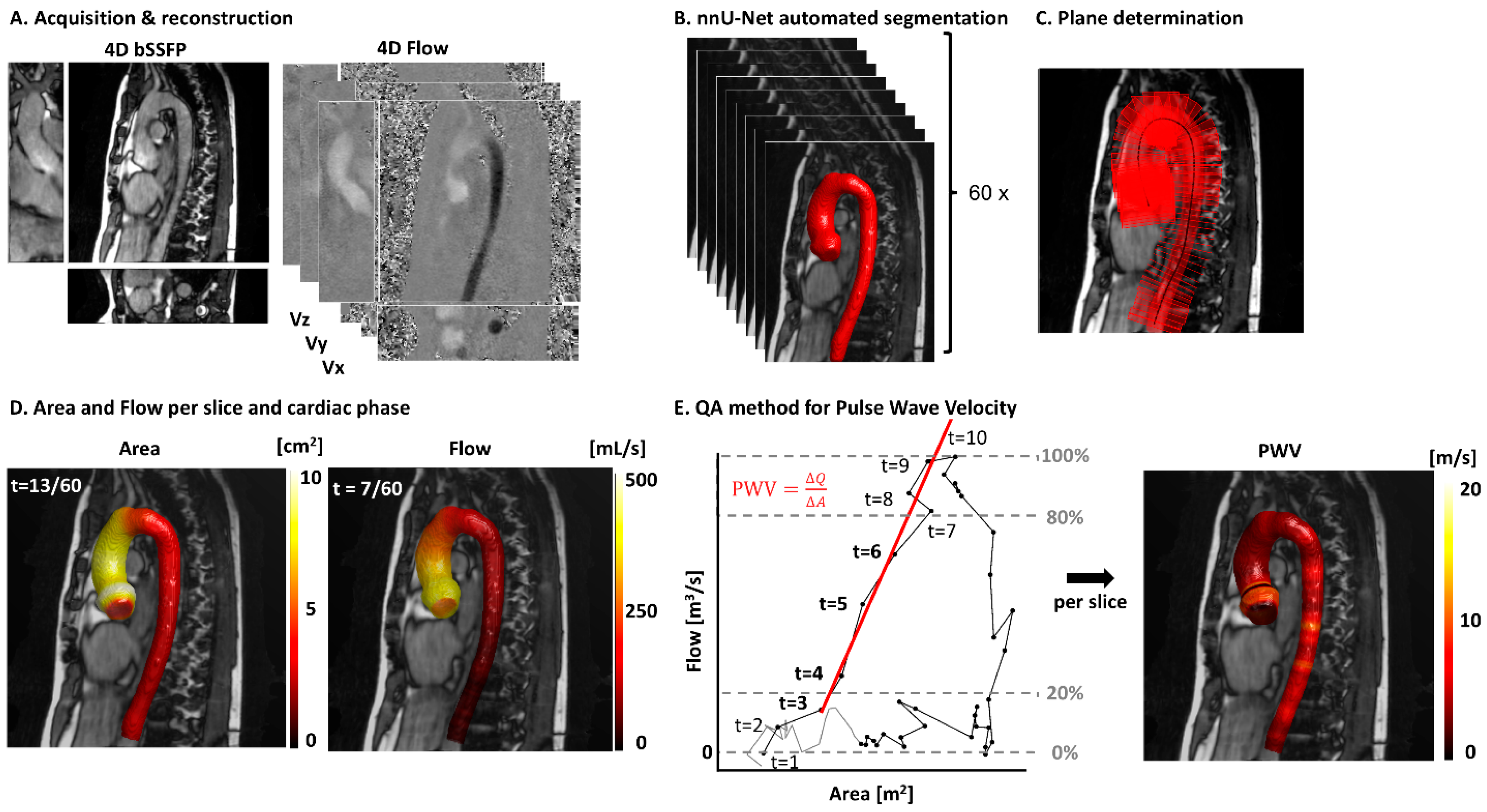
Figure 1. A postprocessing pipeline for local pulse wave velocity (PWV) calculations. (A) A 4D bSSFP and 4D flow of one example volunteer. (B) The automated segmentations of the bSSFP scan acquired after interpolation from 30 to 60 cardiac phases. (C) Segmentation with the centerline. A fifth of the perpendicular planes is shown for clarity. (D) One timeframe of the 4D area and flow values visualized on the aorta segmentation. (E) A representative flow–area (QA) plot for one centerline point and the corresponding plane, with the automated regression point selection method visualized. The bold timeframes (3–6) are used for orthogonal regression. Repeating this for each centerline point results in the PWV map on the right.
Applsci 15 10272 g001
Figure 2. Pulse wave velocity (PWV) measures starting from the root to the descending aorta for all 6 healthy volunteers at scan 1. Raw PWV (gray), raw PWV with R2 > 0.85 (red), and smoothed, interpolated PWV (black) over the length of the thoracic aorta. The mean PWV based on the red line (raw PWV with R2 > 0.85) is indicated with a red striped horizontal line.
Applsci 15 10272 g002
Figure 3. Scan/rescan of healthy volunteer (HV) 1 and scan of Marfan patient 1, from left to right: segmentation with centerline, systolic segmentation with every fifth perpendicular plane (shown on bSSFP), systolic area, systolic flow, and PWV. HV: healthy volunteer.
Applsci 15 10272 g003
Figure 4. A reproducibility analysis of the maximum area, maximum velocity, maximum flow, and pulse wave velocity per centerline location of all six healthy volunteers. The x-axis represents the centerline number, starting from the aortic annulus and progressing towards the distal end of the thoracic aorta.
Applsci 15 10272 g004
Figure 5. Maximum area, maximum velocity, maximum flow, and pulse wave velocity per slice of all six Marfan patients.
Applsci 15 10272 g005
Figure 6. A Bland–Altman graph of PWVWC in comparison with PWVQA. (A) The scan and rescan measurements of the healthy volunteers; each shape corresponds to one subject. (B) Measures for the first scan of the healthy volunteers and those of the Marfan patients, with the shapes indicating to which group a measurement belongs.
Applsci 15 10272 g006
Table 1. Participant characteristics. Numbers are median (Q1–Q3).
Healthy VolunteersMarfan Patients
No. of participants66
Age (y)31 (29–36)30 (28–31)
Female3/6 (50%)3/6 (50%)
Weight (kg)71 (70–74)75 (63–83)
Height (cm)178 (174–183)181 (179–193)
BMI22.7 (21.9–24.2)22.3 (20.4–23.0)
Scan session12
Heart rate (bmp)63 (60–66)59 (53–64)72 (60–79)
Systolic pressure (mmHg)130 (128–132)123 (119–132)132 (130–134)
Diastolic pressure (mmHg)85 (79–88)81 (74–85)81 (78–84)
Disclaimer/Publisher’s Note: The statements, opinions and data contained in all publications are solely those of the individual author(s) and contributor(s) and not of MDPI and/or the editor(s). MDPI and/or the editor(s) disclaim responsibility for any injury to people or property resulting from any ideas, methods, instructions or products referred to in the content.