Just-in-Time Optimal Routing in the Presence of Non-Uniform and Time-Evolving Uncertainty

Abstract

Trajectory planning aims to compute an optimal path and velocity of an agent through the minimization of a cost function. This paper proposes a just-in-time routing method, incorporating the stochastic minimization of a cost function, which ingests the effect of the agent’s environment evolving in space and time. The environment is considered known at present, but the uncertainty increases when advancing in time. To compute the optimal routing in such an uncertain environment, Euler–Lagrange equations will be formulated in a stochastic setting, to obtain a probabilistic optimal planning. With the cost function approximated by using a surrogate modeling based on deep neural networks, a neural formulation of the stochastic Euler–Lagrange equations is proposed and employed.

1. Introduction

Optimal trajectory planning is a topic that arises in many domains of science, engineering, and technology. While reinforcement learning [1,2] is always a valuable route, widely employed in similar settings [3], its two main drawbacks are its high computational cost and the large amount of data required for training purposes.

Previous work [4] proposed an alternative route by employing neural network-based regressions informed by the Euler–Lagrange equation (ELE) for optimal velocity planning along a given path. This procedure was further improved in [5] to compute the optimal trajectory, i.e., both the optimal path and the optimal velocity along it, $\mathbf{x}\left(t\right)$.

In the aforementioned works, the considered cost function includes a term reflecting the effect of the environment (typically wind), which can either assist or resist the agent’s movement. When addressing short paths, it is reasonable to assume that the environment is known and will remain nearly unchanged. Thus, trajectory planning can be elaborated within a deterministic framework, as considered in previous works [4,5].

However, when considering longer trajectories (such as ship routing), currents, sea conditions, and wind, all of which affect the cost function in the optimization problem, are known at the time of planning but are expected to evolve over time, with increasing uncertainty as the time horizon extends. Moreover, ship operations can be scheduled over many months without the possibility of refueling, especially when operating far from homeland.

Similarly, optimal trajectory planning is of utmost importance for airplanes and drones performing missions over extended distances and in foreign territories. In such missions, refueling or recharging is often impossible, while over-fueling can negatively impact the aircraft’s maneuverability. In these situations, especially those occurring far from home bases, environmental conditions such as wind velocity and orientation are only statistically known and are expected to evolve over time, rather than being deterministically available throughout the entire mission duration.

Recently, the hierarchical safe reinforcement learning with prescribed performance control is proposed, where the challenge in unpredictable obstacles is addressed for the leader–follower system. However, these approaches fail to limit travel time for a given path. A solution is proposed in [6], where the authors proposed a finite-time solution, without limiting the path to a fixed interval when possible. Robust optimal tracking is also proposed in [7], using a fixed-time concurrent learning-based actor–critic–identifier.

Other works did attempt the optimal trajectory planing using Gaussian process regressions for small trajectories on robot applications [8,9]. However, the globally optimal solution is often intractable using these techniques, they require trajectory priors, and only a plausible region is identified.

Reinforcement learning is well suited to handle such uncertainty [2,10,11], while traditional ELE formulations are much less so. Nevertheless, the simplicity of applying the ELE, combined with its potential for achieving global optimization, motivates the present research, which proposes extending ELE methods to probabilistic settings, thereby enabling the consideration of evolving uncertainty in optimal trajectory planning [12].

Moreover, many problems in mechanical engineering and manufacturing involve deterministic or stochastic trajectory optimization. For example, motion planning for robotic and mobile systems is investigated in [13]. Other applications involve optimal path identification, such as in 3D printing [14,15,16] and automated tape placement [17,18] using trajectory adjustments along parallel paths. While the authors in [13] use a non-parametric approach for path planning through torque minimization, the other aforementioned methods rely on parametric or spline-based optimization for trajectory planning.

The proposed method has the advantage of being a non-parametric approach guaranteeing a global minimum of the stochastic problem at hand [19,20]. Although it is showcased in this work on routing applications, it can be applied to any path optimization problem, by adapting the functional cost to the selected use case.

Many recent works analyze and propose possible technologies for routing optimization [21,22,23,24]. For example, a hybrid parallel computing scheme combined with an improved inverse distance weight interpolation method was proposed for a search-and-rescue route planning model based on the Lawnmower search method in [21]. The main drawback of that method remains the large span of the domain to be investigated by the optimization algorithm. This drawback is also shared by the authors in [22], who proposed a two-level optimization algorithm for urban routing applied to connected and automated vehicles. Recently, a novel algorithm optimizing routing for multi-modal transport methods in urban settings was proposed, employing a stochastic optimization approach using a generalized interval-valued trapezoidal, in-time, possibility distribution [23]. However, this method does not guarantee on-time arrival or a global optimum, though it can account for disturbances and uncertainties in multi-modal transportation. The method proposed in this work, by contrast, guarantees a global optimum at convergence by minimizing the functional that integrates the cost over the entire travel domain.

This paper begins by exploring the just-in-time routing process, where the objective is to reach the destination within a known time frame. Section 3 then introduces the deterministic neural Euler–Lagrange (ELE) formulation. In Section 4, this deterministic approach is generalized to a stochastic one by combining the neural ELE with a Monte-Carlo sampling strategy and is validated on a use case with a known analytical solution. Section 5 explores several applications and examples, comparing the deterministic and stochastic approaches. Finally, conclusions are presented in Section 6. A list of the used symbols and nomenclature is available in

Table 1. Nomenclature and notations.

Symbol	Name
$\mathbf{x}$	Position vector
x	Position x-coordinate
y	Position y-coordinate
t	Time
$\mathcal{C}$	Instantaneous cost function
$\mathtt{C}$	total cost over a trajectory
ELE	Euler Lagrange Equation
$\mathbf{v}$	Velocity of the object
$v_x$	x-coordinate of $\mathbf{v}$
$v_y$	y-coordinate of $\mathbf{v}$
${\mathbf{v}}_w$	Wind velocity
$v_{wx}$	x-coordinate of ${\mathbf{v}}_w$
$v_{wy}$	y-coordinate of ${\mathbf{v}}_w$
$\dot{o}={\displaystyle \frac{\partial o}{\partial t}}$	Time derivative of o
${\mathcal{NN}}_c$	Neural network approximating $\mathcal{C}$
${\mathcal{NN}}_x$	Neural network identifying $\mathbf{x}$
$\mathit{\mu }$	Vector of mean values
${\mu }^x$	mean value of the x-components
${\mu }^y$	mean value of the y-components
$\Sigma$	Covariance matrix

.

2. Just-in-Time Deterministic Routing

The path is assumed starting at ${\mathbf{X}}_0$ at $t=0$, and should finish at position ${\mathbf{X}}_T$ at time $t=T$. At its turn, the local cost function $\mathcal{C}$ is assumed depending on the difference of velocities between the one of the agent $\dot{\mathbf{x}}$ and the one of the environment ${\mathbf{v}}_w$ at the agent’s position $\mathbf{x}\left(t\right)$.

The total cost $\mathtt{C}$ reads

$$\mathtt{C}={\int }_0^T\mathcal{C}(t,\dot{\mathbf{x}}\left(t\right),{\mathbf{v}}_w\left(\mathbf{x}\left(t\right)\right))dt.$$

(1)

In what follows, for the sake of illustration, we consider three different scenarios.

2.1. Constant Environment Effect

We consider in this case the one-dimensional case $x\left(t\right)$ with $X_0=0$, at $t=1$, and $X_T=1$, with $T=1$, and $\mathcal{C}={(\dot{x}-v_w)}^2$, that is, $\mathcal{C}={\dot{x}}^2+v_w^2-2v_w\dot{x}$.

The selected boundary conditions are chosen without any loss of generality. Now, the ELE,

$${\displaystyle \frac{\partial \mathcal{C}}{\partial x}}-{\displaystyle \frac{d}{dt}}\left({\displaystyle \frac{\partial \mathcal{C}}{\partial \dot{x}}}\right)=0,$$

(2)

leads to $\ddot{x}=0$, which, integrated twice, results in $x\left(t\right)=a+bt$, which, taking into account the initial and final conditions, reduces to $x\left(t\right)=t$, with a constant velocity $\dot{x}=1$, independent of the the value of $v_w$. That is, for any value of $v_w$, the minimum cost enabling the fulfillment of both the initial and final conditions is the constant unit velocity.

2.2. Environment Effect Evolving in Time

Here we consider the same case as before, with the only difference being the environment effect that now grows in time, that is $v_w=t$. Thus, $\mathcal{C}={(\dot{x}-t)}^2={\dot{x}}^2+t^2-2t\dot{x}$, inserted into the ELE, leads to $\ddot{x}=1$, whose solution $x\left(t\right)={\displaystyle \frac{t^2+t}{2}}$ implies the velocity $\dot{x}\left(t\right)=t+{\displaystyle \frac{1}{2}}$, where the agent profits from the environment effect by increasing its velocity in time.

2.3. Environment Effect Evolving in Space

This section consider $v_w=x$, which implies $\mathcal{C}={(\dot{x}-x)}^2$, which, inserted into the ELE, leads to $\ddot{x}=x$, whose solution reads $x\left(t\right)=a{e}^t+b{e}^{-t}$, with the value of constants a and b determined by the initial and final conditions $x\left(0\right)=0$ and $x\left(1\right)=1$.

2.4. Discussion

It is also important to mention that, in the case of the just referred time-dependent environment, changing $v_w=t$ to $v_w=-t$ changes both the $x\left(t\right)$ and the velocity along it. However, in the space-dependent case, when changing $v_w=x$ by $v_w=-x$, nothing changes.

For more complex environments, the resulting ordinary differential equation (ODE) can be solved by discretizing it by using typical discretization techniques, for example, the finite differences. However, sometimes the cost function is unknown analytically, and is approximated using a surrogate model, like a neural network

$$\mathcal{C}={\mathcal{NN}}_c(\dot{x},x,t),$$

(3)

where x or t could be absent in some particular cases. Such a cost function is determined during the agent calibration, in a wind tunnel, for example, in the case of drones, but it could also be obtained from high-fidelity solutions of aerodynamic or/and hydrodynamic software.

3. Neural Euler–Lagrange Formulation

With the cost expressed by the pre-trained neural network (3), we assume that the trajectory results from a trainable neural network

$$x={\mathcal{NN}}_x\left(t\right),$$

(4)

whose time derivative leads to the velocity $\dot{x}$, with x, $\dot{x}$, and the time t being the inputs of the cost neural network (3).

To train the network (4), it suffices to use the ELE residual as the cost function, whose derivatives can be easily computed by automatic differentiation.

4. Addressing Uncertainty

This section considers the time evolution of the environment uncertainty. As soon as its statistical distribution is defined, a sampling consisting on N realizations can be performed. Then, a cost ${\mathcal{C}}_i$ is associated with each realization $i=1,...,N$.

At first view, the stochastic formulation reduces to the solution of N deterministic Euler–Lagrange equations by using the neural formulation introduced in the previous section, to compute the trajectory statistics from all the solutions.

Another possibility, specially adapted to the use of neural architectures, consists of training the network ${\mathcal{NN}}_x$ with a loss function that considers the N ELE residuals.

By defining the residual ${\mathcal{R}}_i$ for realization i using

$${\mathcal{R}}_i\equiv {\displaystyle \frac{\partial {\mathcal{C}}_i}{\partial x}}-{\displaystyle \frac{d}{dt}}\left({\displaystyle \frac{\partial {\mathcal{C}}_i}{\partial \dot{x}}}\right),$$

(5)

the global loss $\mathcal{L}$ considered in the training reads

$$\mathcal{L}=\sum _{i=1}^N{\parallel {\mathcal{R}}_i\parallel }^2.$$

(6)

Numerical Validation in the Deterministic Case

First we consider the deterministic 2D case with $\mathbf{x}={(x,y)}^T$ and ${\mathbf{v}}_w=\mathbf{x}$. The initial and final conditions are given by ${\mathbf{X}}_0=\mathbf{0}$ and ${\mathbf{X}}_T={(1,1)}^T$, at time $t=T=1$. The cost is assumed to be the one introduced in Section 2.3, and given by

$$\mathcal{C}=\parallel \dot{\mathbf{x}}{-\mathbf{x}\parallel }^2.$$

(7)

This cost function $\mathcal{C}$ is used to generate data, and to train a neural network surrogate approximating the cost:

$${\mathcal{NN}}_c(\dot{\mathbf{x}},\mathbf{x})\approx \mathcal{C},$$

(8)

which should replicate that cost function after the appropriate training.

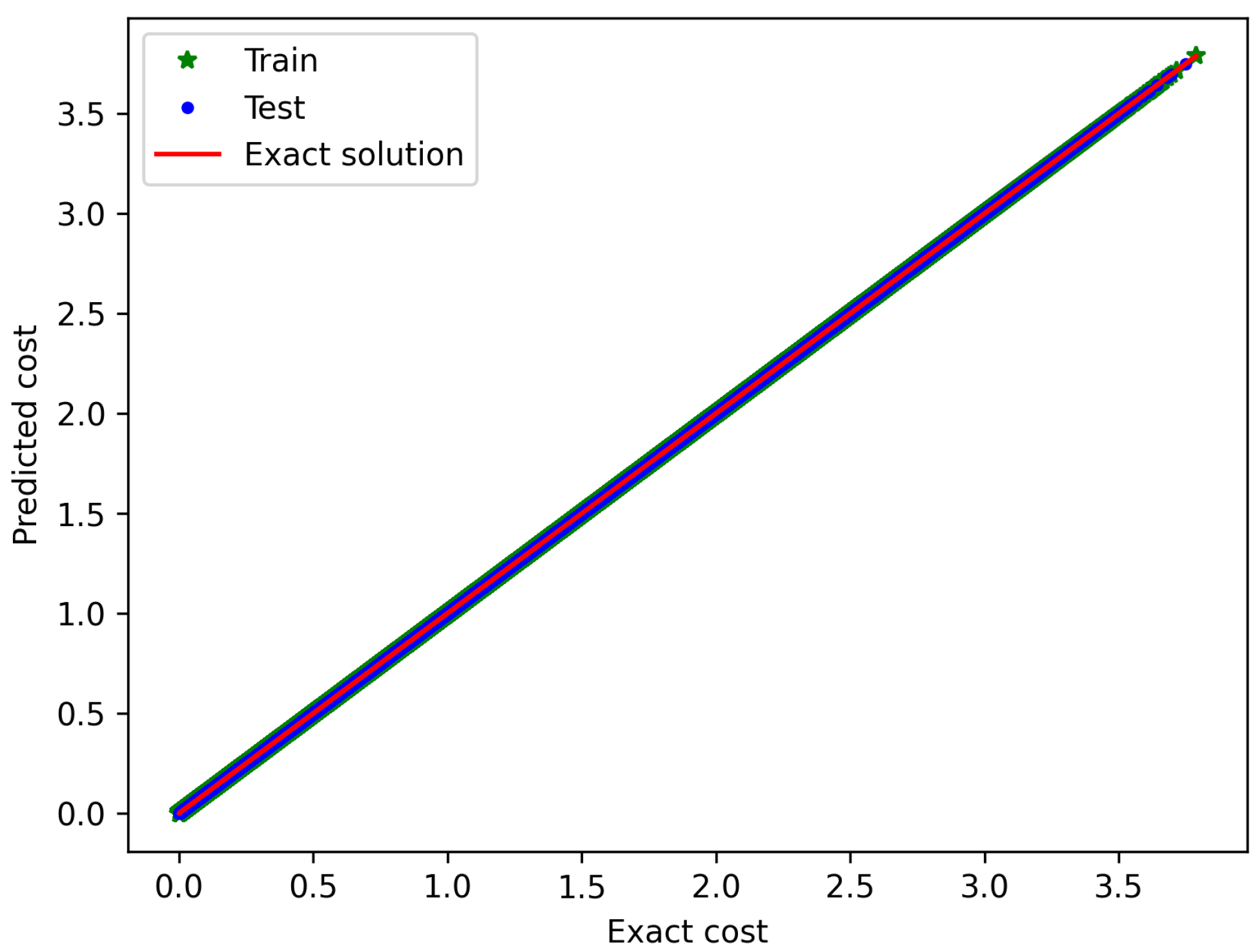
First, 50 million combinations $(\dot{\mathbf{x}},\mathbf{x})$ were considered for training the cost network $\mathcal{C}={\mathcal{NN}}_c(\dot{\mathbf{x}},\mathbf{x})$, $80\%$ of which were used in the training. The remaining $20\%$ were used to test the trained model.

Figure 1 depicts the prediction (8) versus the reference value (7) of the cost function, from which an almost perfect training can be concluded (the $R^2$ metrics is higher than 0.99 for both the training and the test datasets, with an absolute percentage error lower than ${10}^{-7}$ on both datasets).

Once the cost network ${\mathcal{NN}}_c$ is trained, the network ${\mathcal{NN}}_x$ providing the optimal trajectory can be trained with the loss associated with the ELE residual as previously discussed. The used network for ${\mathcal{NN}}_c$ is a three-layer dense network with size (200, 60, 60, 60, 1) and activations (tanh,relu,relu,rely,linear), respectively. 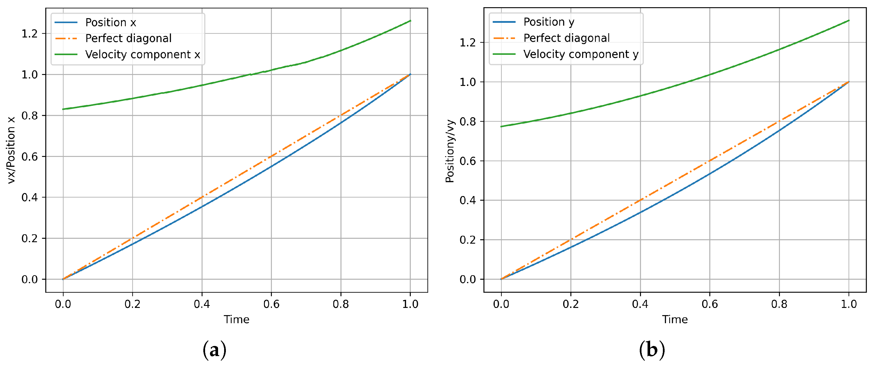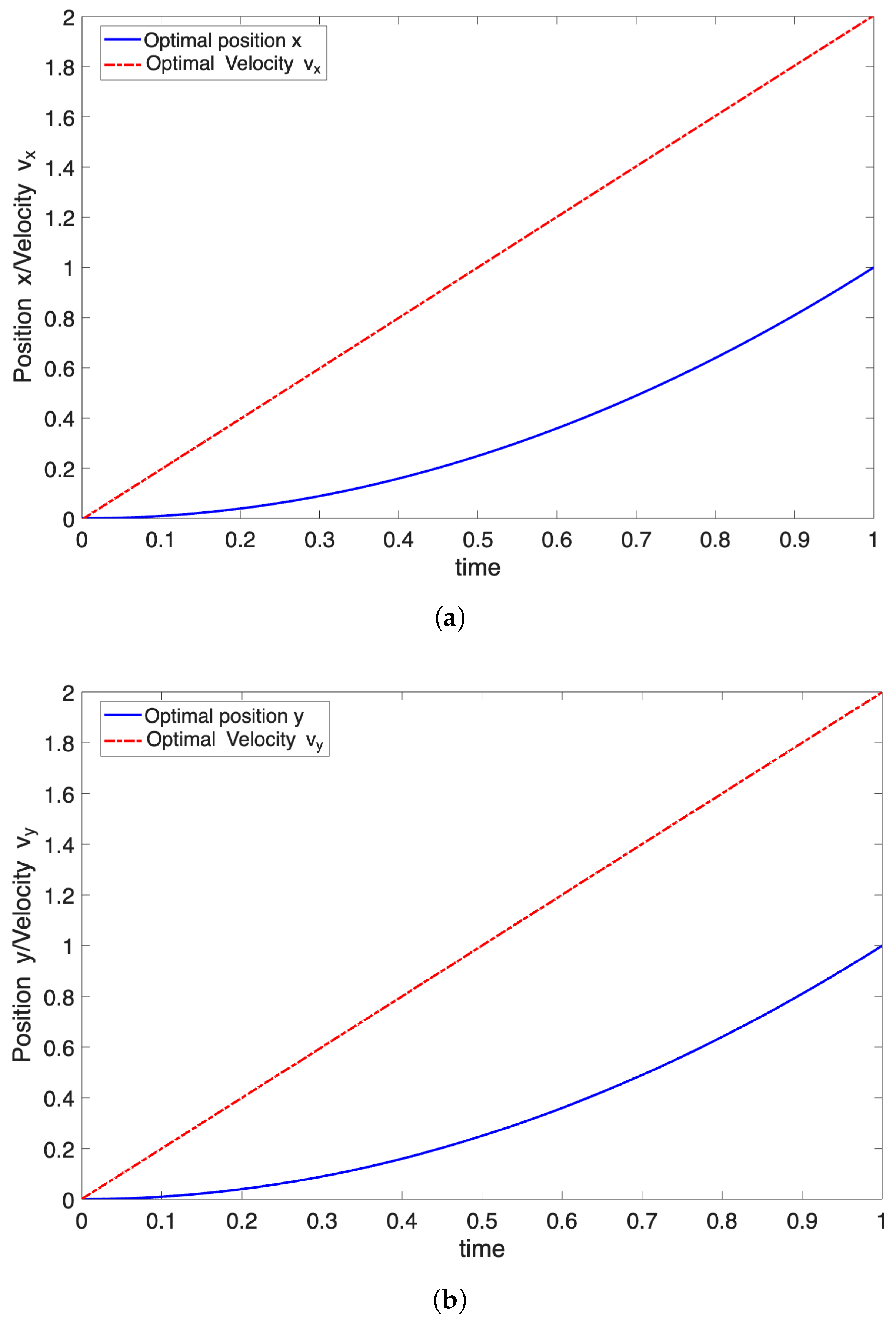Two different networks of identical structure are used to predict the x and y coordinates of the path. The resulting optimal trajectory is depicted in Figure 2 for both the x and the y coordinate. Figure 2 also depicts the resulting optimal velocity.

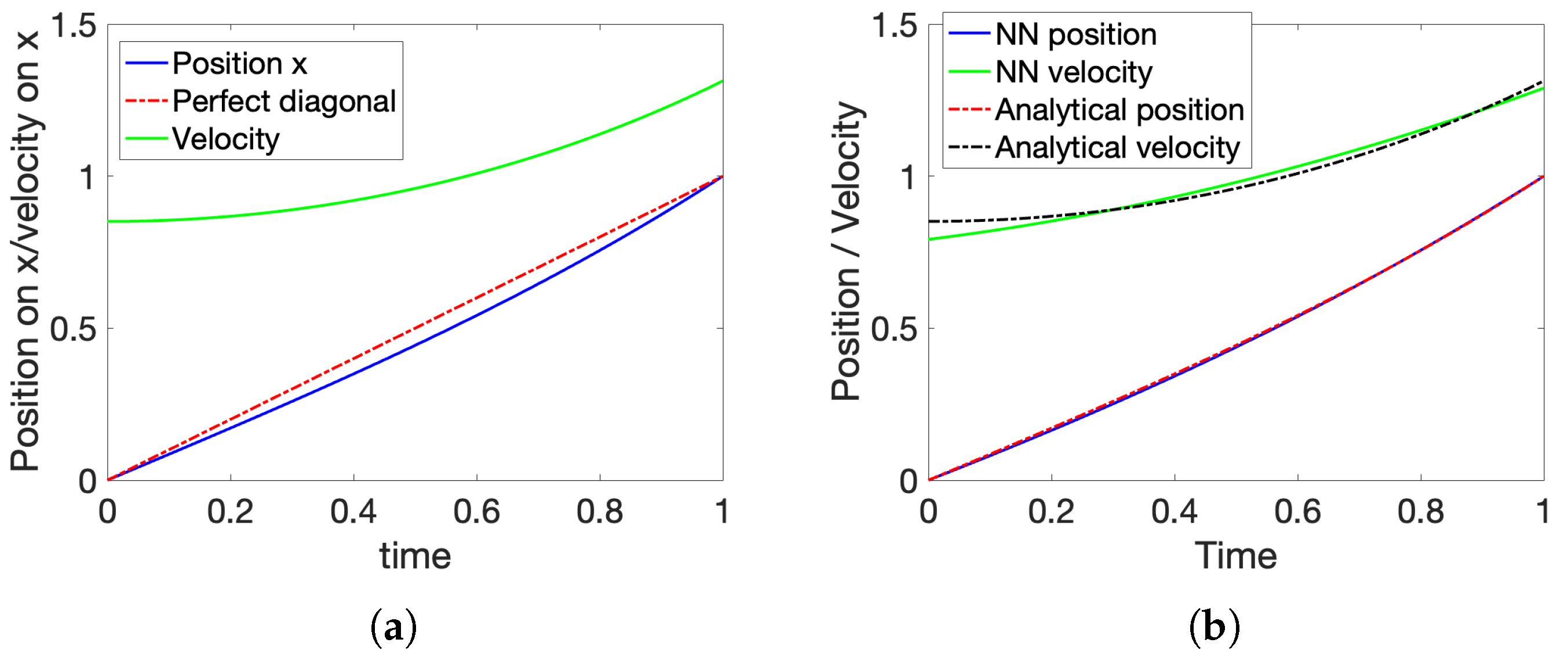
In the present case, the problem admits an analytical solution that serves as a reference solution to validate the approach. Another possibility to validate the results in the present case, in which the cost function has an explicit expression, consists of solving the ELE by employing any discretization technique, like the finite differences methods.

The problem’s analytical solution is shown in Figure 3 along with a comparison to the one identified by the trained network. The relative and absolute errors between the analytical solutions and the one provided by the neural approach are shown in Figure 4. Figure 4 demonstrates the high accuracy of the proposed planning procedure.

5. Numerical Results in a Stochastic Setting

In the following examples, we consider the cost function defined by

$$\mathcal{C}={∥\dot{\mathbf{x}}-{\mathbf{v}}_w∥}^2.$$

(9)

However, now the wind velocity ${\mathbf{v}}_w$ becomes stochastic, having different expressions depending on the considered use case. In all the illustrated examples in this section, Tensorflow is used in the implementation [25]. The training of the neural network ${\mathcal{NN}}_x$ minimizing the stochastic ELE cost function is performed using an ADAM stochastic gradient descent algorithm [26], with a custom decreasing learning rate from ${10}^{-3}$ to ${10}^{-6}$ over the course of 1000 epochs. The learning starts with batches of 50 points over the trajectory and increases over the epochs to end with a learning over the full trajectory. The trajectory’s boundary conditions are imposed by construction using a change of variables. The same neural network architecture is also used for ${\mathcal{NN}}_x$. In this section, we also refer to the agent’s velocity $\dot{\mathbf{x}}$ by $\mathbf{v}$, of components $(v_x,v_y)$.

In the rest of this section, the potential wind trajectories are sampled a priori. Later on, each sampled potential wind history is treated as a deterministic sample.

5.1. A First Example with a Sampled Multi-Normal Wind Velocity Distribution

This section assumes a uniform environment, whose uncertainty evolves in time. Thus, the environment statistics is assumed to follow a multi-normal distribution, with the dimensionality given by a partition of the time interval. If we consider a partition defined by M nodes uniformly distributed on the time interval $[0,T]$, with the partition length $h=T/(M-1)$, the nodal times become

$$t_i=(i-1)·h,i=1,...,M.$$

(10)

The multi-normal statistic becomes fully determined using the $M\times M$ cross-correlation matrix $\Sigma$, and the $M\times 1$ mean-vector $\mathit{\mu }$.

Here, without loss of generality, we consider a linear evolution of the components of vector $\mathit{\mu }$:

$${\mu }_i=a+b{t}_i,$$

(11)

with the diagonal components of $\Sigma$ (variances) also following a linear evolution in time, according to

$${\Sigma }_{i,i}=c+d{t}_i,$$

(12)

with the covariance scaling (inversely) with the distance in time according to

$${\Sigma }_{ij}=e^{{\displaystyle \frac{-{(t_i-t_j)}^2}{2{\beta }^2}}}.$$

(13)

In the cases addressed below, the values $c=1$, $d=0.5$, and $\beta =10$ are considered. Now, by sampling the multi-normal distribution defined above, different trajectories of the stochastic process at the time nodes are obtained. From them, a spline can be used for determining the value in between the nodes.

In this example, the x- and y-components of vector $\mathit{\mu }$ are given by

$$\left\{\begin{array}{c}{\mu }_j^x=20t_j\hfill \\ {\mu }_j^y=20t_j\hfill \end{array}\right.,i=1,\dots ,M.$$

(14)

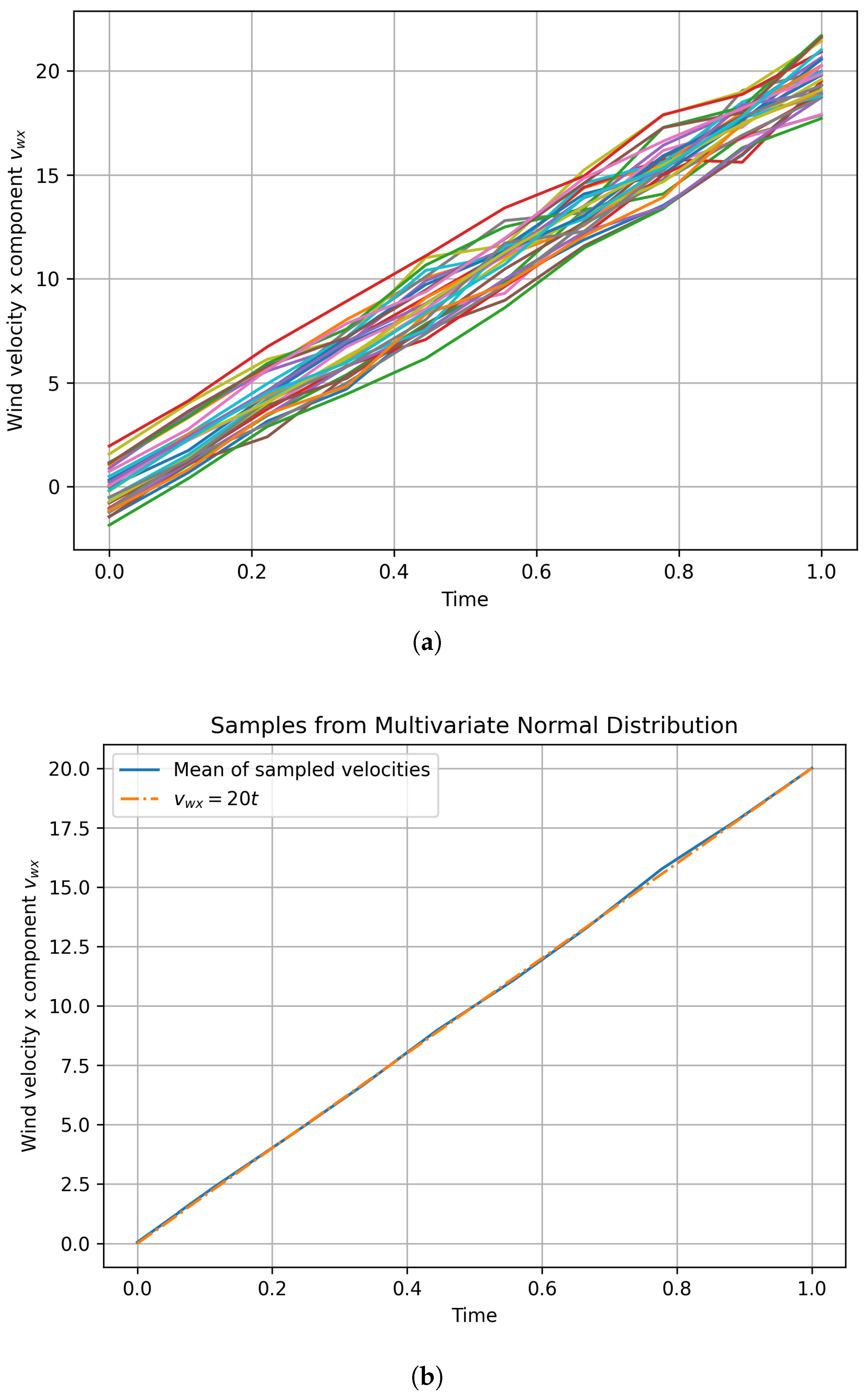
We considered 30 realizations of the multi-normal distribution illustrated (without considering a spline-based smoothing) in Figure 5. The computed results following the rationale described in Section 4, to address uncertainty quantification, are illustrated in Figure 6.

5.2. A Second Case-Study Considering a Markov Chain Monte-Carlo Sampling

In this second example, the change in time of the wind velocity is sampled by using the Metropolis–Hastings algorithm, a powerful Markov chain method to simulate multivariate distributions [27].

This section considers two cases: (i) a symmetrical probability distribution of the wind velocity in terms of amplitude and orientation, and (ii) another case where the probability distribution is slightly asymmetrical, while conserving the same mean and standard deviation.

In both sampling efforts, the sampled probability is normal of the mean $\left(20\sqrt{2}\right)t$ for the wind velocity magnitude $\parallel {\mathbf{v}}_w\parallel$ and a standard deviation of $0.2$. Regarding the orientation $\theta$, the sampled probability is normal with a mean of ${45}^{°}$ and a standard deviation of $0.2$. However, for both the velocity magnitude and orientation, the acceptance probability is normal of the mean $|q_{sampled}-q_{current}|$ and a standard deviation of $0.2$ in the symmetric case, while in the asymmetrical one, the acceptance probability is a lognormal distribution of the same mean and standard deviation, the quantity q being either the wind velocity amplitude $\parallel {\mathbf{v}}_w\parallel$ or the wind orientation $\theta$. Both sampling of the wind velocity magnitude and its orientation are performed independently, and the wind vector components are computed using

$$\left\{\begin{array}{c}{v}_{wx}=\parallel {\mathbf{v}}_w\parallel cos\left(\theta \right)\hfill \\ v_{wy}=\parallel {\mathbf{v}}_w\parallel sin\left(\theta \right)\hfill \end{array}\right.$$

(15)

Using the symmetrical and asymmetrical probability density functions, we construct 30 wind velocity samples in each use case. The sampled wind velocities along x and y are illustrated in Figure 7 along with their mean distribution.

The agent’s trajectory (path and velocity) are optimized using the cost function defined in Equation (9). The solutions obtained using the Euler–Lagrange-based stochastic procedure are illustrated in Figure 8 for the symmetric and asymmetric cases.

5.3. Discussion on the Stochastic Approaches

The present section compares the stochastic approaches using the different sampling techniques, along with a deterministic approach. The selected deterministic solution is the one minimizing the cost for the mean value of the distribution using the deterministic $ELE$ framework. For instance, in this example, the deterministic solution is the optimal path for a deterministic environment where the wind velocity is defined by

$$\left\{\begin{array}{c}{v}_{wx}=20t\hfill \\ v_{wy}=20t,\hfill \end{array}\right.$$

(16)

which consists of the theoretical mean distribution of the wind considered in Section 5.1 and Section 5.2.

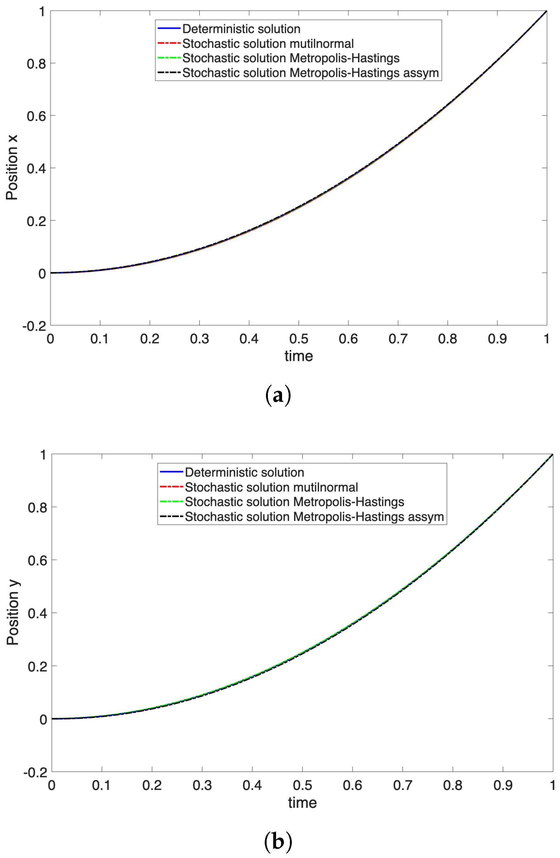
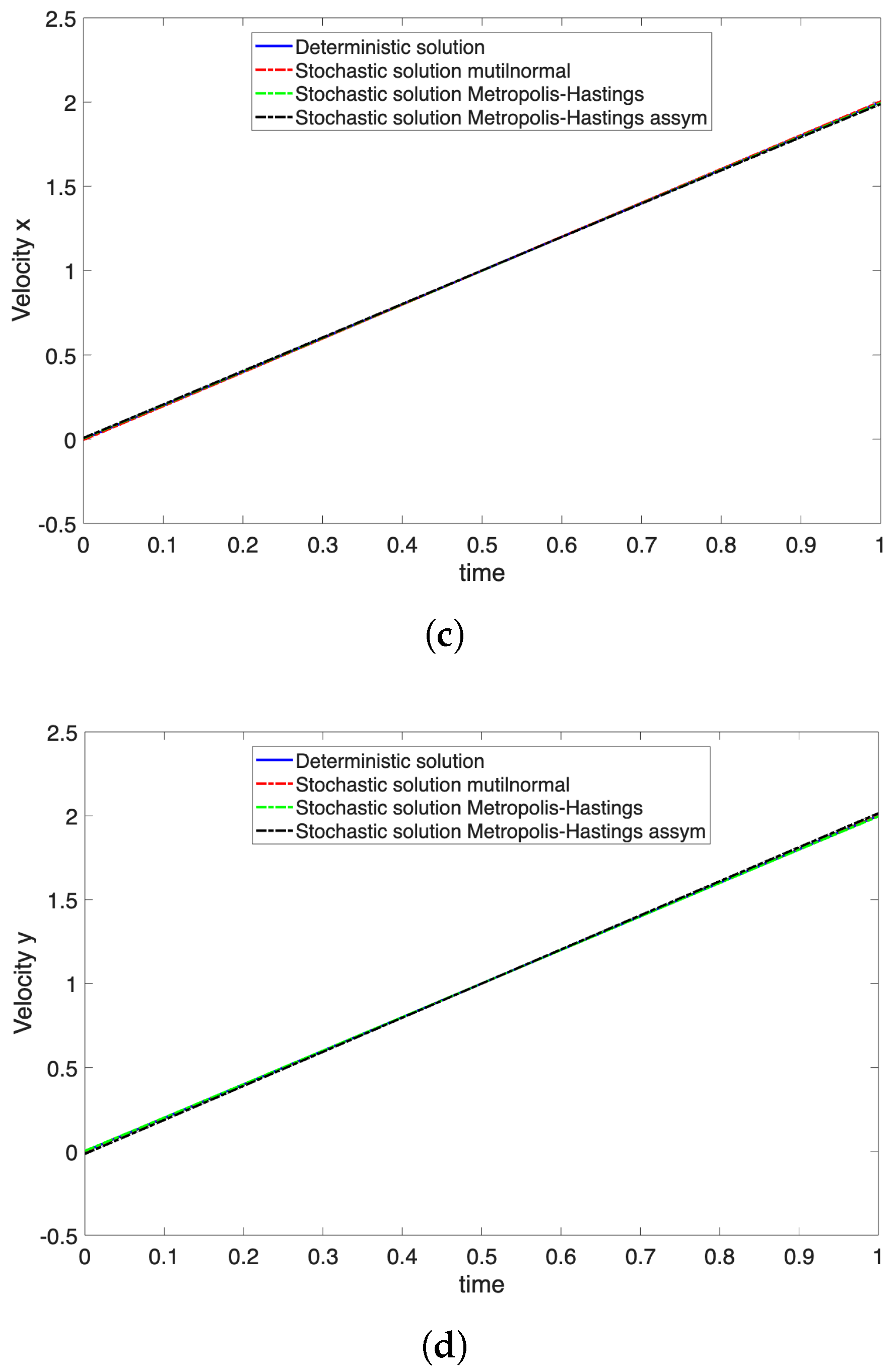
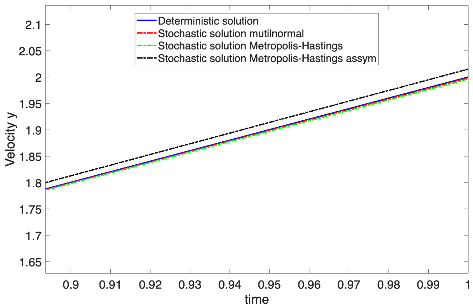
Figure 9 compares the optimal path in terms of x and y coordinates, as well as $v_x$ and $v_y$, for different distributions. Figure 10 shows a zoom on the identified paths. From it, we can conclude that the deterministic solution using the wind average is comparable to the probabilistic solutions, with the difference becoming more noticeable for the asymmetrical probability density functions, the nonlinearities involved in the procedure being more significant. In general, minimizing the cost for the mean value of the wind velocity in the treated examples is not optimal with respect to the cost that each wind velocity sample entails.

5.4. Considering Available Wind Velocity Statistics

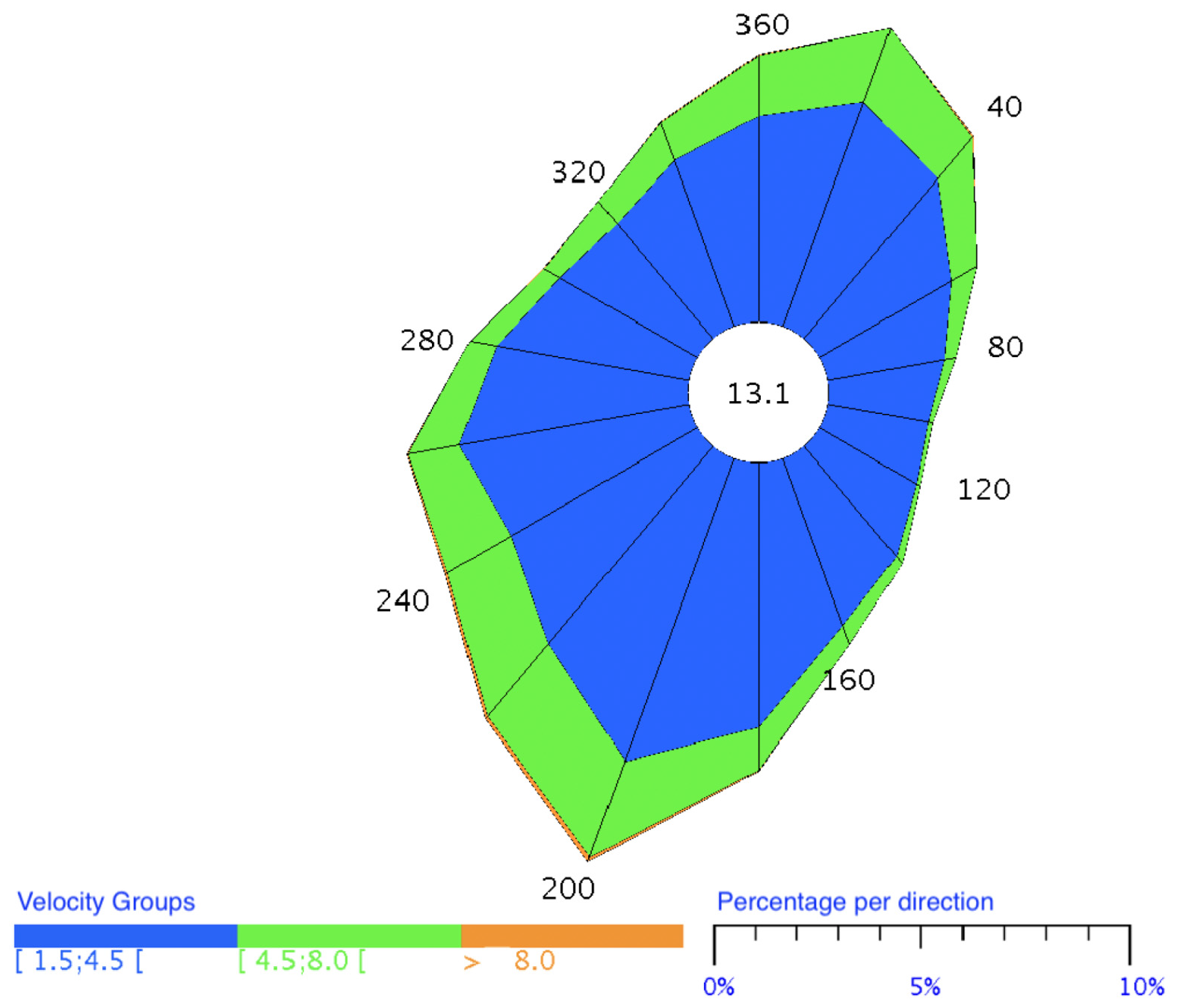
This section considers the wind probability distribution in the city of Paris [28] shown in Figure 11.

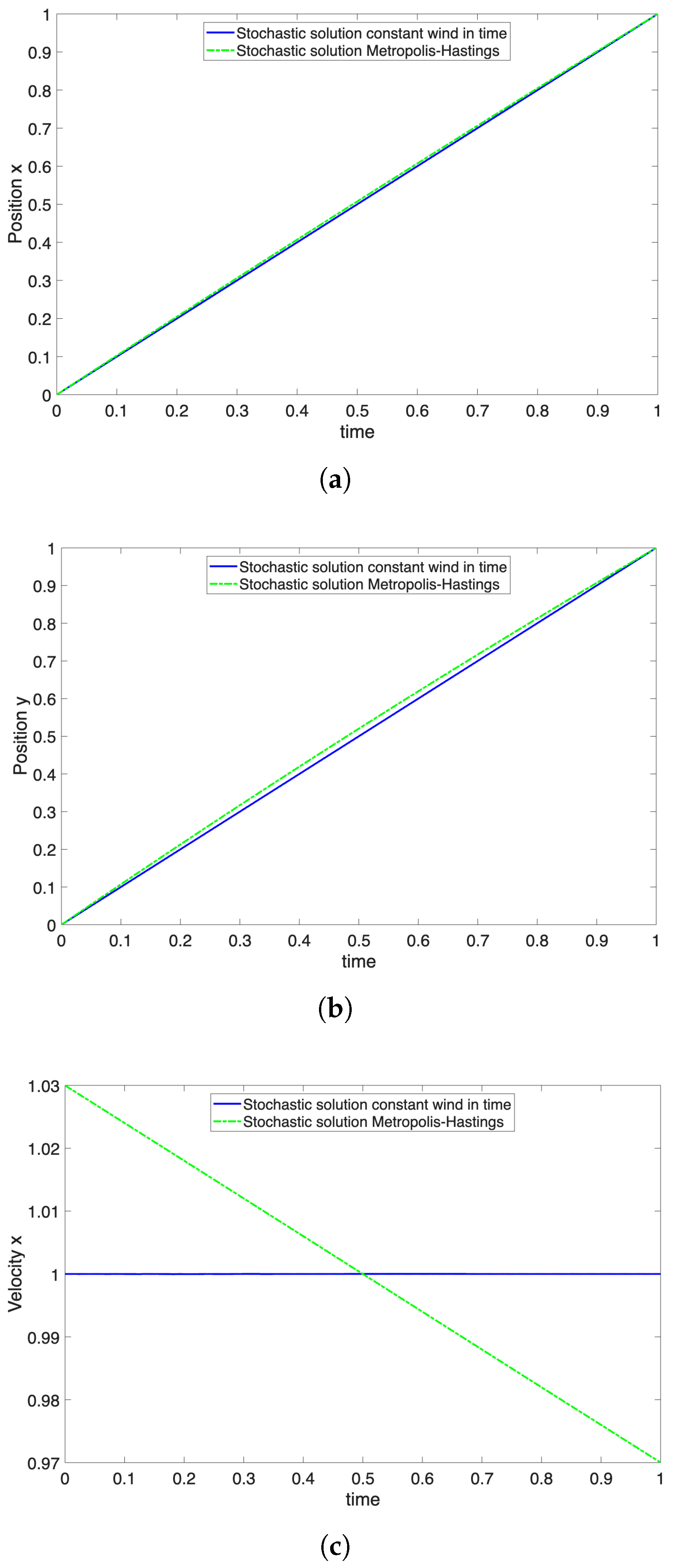
The wind distribution is sampled for two cases. First set of 30 samples uses constant values along the selected time frame of one hour, picked using the probability distribution illustrated in Figure 11. The second set of 30 samples is obtained using the Metropolis–Hastings sampling algorithm, with a sampling evolution every minute. The optimal trajectory results are illustrated in Figure 12 for both cases.

We can note a slight difference between the different sampling procedures. A deterministic solution considering the average values of the wind velocity remains very close to the sampling of constant velocities in time shown in Figure 12.

6. Conclusions

This work extends former proposals of computing optimal trajectories from a neural network approximation trained to minimize the Euler–Lagrange equation residual as a loss function. This extension into the stochastic setting in which the environment varies in space and its uncertainty evolves in time allowed addressing stochastic environmental evolution during routing operations using the proposed ELE framework.

The proposed strategy consists of the statistical modeling of the uncertainty, which is then sampled using a Monte-Carlo procedure. Later, the network provides the optimal trajectory trained from a loss that considers the Euler–Lagrange equation residual associated with the different stochastic process realizations.

The numerical examples enabled the procedure validation as well as comforting on the procedure simplicity. The results showcase a difference between deterministic approaches considering only the mean values of the stochastic realizations, and the EL stochastic approach using Monte-Carlo minimization of the stochastic ELE form, even if for the simplistic cases addressed, the difference is not significant. In the case where the cost function $\mathcal{C}$ is linear, there is no difference between the deterministic solution considering the average of the environmental effect, and the proposed work where we consider the stochastic minimization of the cost function. On the contrary, when $\mathcal{C}$ is highly non-linear, the effect becomes more pronounced.

It is important to emphasize the zero-data framework used in this routing process. No experimental nor simulated data is needed for the network training, as the network learns the optimal solution from the Euler–Lagrange residual minimization, in contrast with the vast majority of the available techniques in the literature.

The proposed work can be extended to add the availability of obstacles and dynamically evolving obstacles. Moreover, the assessment of the Monte-Carlo sampling size and the convergence analysis of the proposed Euler–Lagrange framework will be analyzed.