Synergistic Remote Sensing and In Situ Observations for Rapid Ocean Temperature Profile Forecasting on Edge Devices

Abstract

Regional rapid forecasting of vertical ocean temperature profiles is increasingly important for marine aquaculture, as these profiles directly affect habitat management and the physiological responses of farmed species. However, observational temperature profile data with sufficient temporal resolution are often unavailable, limiting their use in regional rapid forecasting. In addition, traditional numerical ocean models suffer from intensive computational demands and limited operational flexibility, making them unsuitable for regional rapid forecasting applications. To address this gap, we propose PICA-Net (Physics-Inspired CNN–Attention–BiLSTM Network), a hybrid deep learning model that coordinates large-scale satellite observations with local-scale, continuous in situ data to enhance predictive fidelity. The model also incorporates weak physical constraints during training that enforce temporal–spatial diffusion consistency, mixed-layer homogeneity, and surface heat flux consistency, enhancing physical consistency and interpretability. The model uses hourly historical inputs to predict temperature profiles at 6 h intervals over a period of 24 h, incorporating features such as sea surface temperature, sea surface height anomalies, wind fields, salinity, ocean currents, and net heat flux. Experimental results demonstrate that PICA-Net outperforms baseline models in terms of accuracy and generalization. Additionally, its lightweight design enables real-time deployment on edge devices, offering a viable solution for localized, on-site forecasting in smart aquaculture.

1. Introduction

Ocean temperature profiles describe the vertical thermal structure of ocean waters and provide detailed information on variations across the mixed layer, thermocline, and bottom waters [1,2,3]. These profiles are crucial in fisheries and aquaculture because they directly influence subsurface habitat conditions, prey availability, and water column stability, all of which affect the growth and health of farmed species [4,5,6]. Regional rapid forecasting of temperature profiles is therefore increasingly important for adaptive aquaculture management [7,8]. Regions such as the Yellow Sea Cold Water Mass, characterized by persistent bottom–surface thermal differences, are sensitive habitats for species such as scallops and sea cucumbers, whose physiological stress correlates with bottom temperature fluctuations [9,10].

Therefore, regional rapid forecasting of vertical temperature evolution helps aquaculture practitioners adjust cage depths, optimize feeding, and mitigate risks from extreme events [11,12]. High-resolution, physically consistent, and timely models are increasingly important for smart aquaculture and ecological risk management.

However, ocean temperature profiles evolve under complex physical processes [13,14], influenced by surface factors like wind and heat flux as well as multi-scale interactions involving salinity, turbulence, and deep circulation [15]. In regions with intricate thermal structures, such as the Yellow Sea, nonlinear dynamics lead to abrupt structural shifts [16], further complicated by weather variability, small-scale turbulence, and ecological events [17]. Accurately capturing these rapidly varying, nonlinear vertical dynamics, especially at hourly scales, remains a key scientific and technical challenge.

While numerical models remain foundational in ocean prediction, they face limitations in real-time applications. High computational costs, sensitivity to initial conditions, and difficulty in deployment of edge devices limit their responsiveness in localized applications that require frequent updates. They have limited capacity to learn from real-world data, particularly under sparse observations.

Recent advances in satellite remote sensing, reanalysis products, and deep learning provide promising alternatives. Satellite data offer key physical variables such as SST, wind fields, and sea surface height anomalies, while deep learning excels at spatiotemporal modeling and is well-suited for edge deployment [18]. Several studies have applied data-driven methods. LSTM has been used to predict mixed-layer temperatures from meteorological inputs [19]; the effectiveness of LSTM in SST forecasting was demonstrated in [20]; a multi-layer ConvLSTM was proposed for 3D ocean temperature modeling [21]; a 4D CNN (SST-4D-CNN) was developed for thermocline prediction [22]; SST, ZOS, and wind fields have been fused to enhance subsurface forecasts [23]; and CNN–LSTM–attention architectures integrating temperature, salinity, ocean currents, and MLD have demonstrated the value of embedding physical drivers [24].

Despite these advances, several challenges persist in current ocean temperature modeling approaches. Traditional numerical models, while physically grounded, often require high computational resources and are difficult to adapt for localized applications requiring frequent updates. Many models use input data updated only daily or less frequently, hindering regional rapid forecasting. Most models do not explicitly incorporate physical constraints, which reduces their interpretability. Most existing studies also focus on 2D SST prediction without full-profile modeling, which limits practical applicability.

To overcome these challenges, this study leverages the synergy between large-scale satellite data and fine-scale, continuous in situ observations. We propose a deep learning model, namely PICA-Net, which combines 1D-CNN for vertical structure extraction, BiLSTM for temporal dynamics, and attention mechanisms for adaptive feature weighting [25,26]. Using hourly historical data, it predicts temperature profiles at 6 h intervals over the next 24 h. Inputs include satellite-derived variables and physical drivers.

To improve physical coherence, the model incorporates additional physical constraint terms—including temporal–spatial diffusion consistency, mixed-layer homogeneity constraint, and surface heat flux consistency constraint—into its loss function [27]. Trained on reanalysis data, the model shows strong accuracy and generalization, and incorporating physical constraints further improves shallow-layer coherence and physical realism. Together, they demonstrate the complementary strengths of data-driven and physics-informed approaches.

The reanalysis data we used (e.g., CMEMS, ERA5) assimilate multiple in situ sources such as Argo float profiles, ship-based measurements, and other observational platforms, after rigorous quality control. Reanalysis products are adopted as ground truth for their temporal–spatial continuity and alignment with known ocean dynamics, serving as reliable substitutes for in situ data [28]. This lays the foundation for future integration of real-time observations, advancing responsive and accurate temperature forecasting systems.

Ultimately, PICA-Net supports edge deployment, enabling real-time, site-specific forecasting to guide smart aquaculture decisions. It offers robust support for scheduling, environmental alerts, and precision operations. The remainder of this paper is structured as follows: Section 2 presents the data sources and preprocessing; Section 3 details the PICA-Net architecture and physical constraints; Section 4 describes the experimental setup and results, including ablation studies and edge deployment; and Section 5 concludes with future directions for real-time integration and model generalization.

2. Materials and Methods

2.1. Data

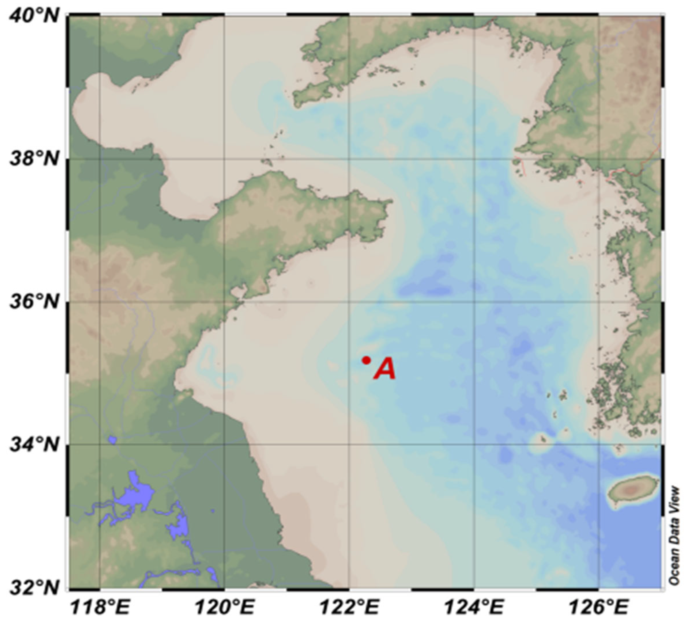
This study focuses on a representative aquaculture region in the Yellow Sea, China, located at 122.26° E, 35.16° N. The area is influenced by the Yellow Sea Cold Water Mass, monsoonal wind fields, and air–sea heat exchange, resulting in pronounced vertical thermal stratification and seasonal thermocline variations. As a typical zone of dynamic marine thermal evolution, it holds both scientific importance and practical relevance for temperature profile prediction. The study area is shown in Figure 1 below:

2.1.1. Data Sources and Variable Descriptions

We constructed a high-resolution dataset by integrating satellite remote sensing and reanalysis products from CMEMS and ERA5, which assimilate diverse satellite and buoy observations to ensure physical consistency and temporal continuity. These reanalysis datasets currently serve as reliable substitutes for in situ measurements in model training and evaluation. Their proven accuracy and coherence make them suitable for building generalizable models, while also laying a foundation for future integration of real-time site-specific sensor data (

Table 1. Physical variables input into the model and their sources.

Variable Name	Description	Data Source	Data Type	Temporal Resolution	Unit
${\theta }_o$	Temperature profile	CMEMS	Reanalysis (remote-sensing blended)	6 h	°C
$S_o$	Salinity profile	CMEMS	Reanalysis	6 h	PSU
$u_o$$,v_o$	Ocean current velocity (u, v)	CMEMS	Reanalysis	6 h	m/s
$\eta$	Sea surface height anomaly	CMEMS	Reanalysis (satellite altimetry)	1 h	m
$h_{mld}$	Mixed-layer depth	CMEMS	Reanalysis (model-derived)	1 d	m
$u_{10},v_{10}$	10 m wind components (u, v)	CMEMS	Reanalysis (satellite + in situ)	1 h	m/s
${\tau }_x,{\tau }_y$	Wind stress components	CMEMS	Reanalysis	1 h	N/m2
$R_{ld}$	Downward longwave radiation	ERA5	Reanalysis	1 h	W/m2
$R_{sd}$	Downward shortwave radiation	ERA5	Reanalysis	1 h	W/m2
$Q_s$	Sensible heat flux	ERA5	Reanalysis	1 h	W/m2
$Q_l$	Latent heat flux	ERA5	Reanalysis	1 h	W/m2
$T_{\mathrm{S}\mathrm{S}\mathrm{T}}$	Sea surface temperature	ERA5	Reanalysis (satellite-dominated)	1 h	°C

).

2.1.2. Dataset Composition and Preprocessing Workflow

The dataset used in this study spans from 1 May 2023 to 20 May 2025, comprising a total of 18,001 hourly records. Based on a fixed temporal split, the data is divided into a training set and a validation set. The training set covers the period from 1 May 2023 to 20 December 2024, totaling 14,400 h, while the validation set spans from 21 December 2024 to 20 May 2025, comprising 3601 h. No separate test set was used in this study. All experimental results were reported on the validation set, which was held out entirely during training. This setup ensures that model performance is evaluated on unseen data, thereby preserving the integrity of the evaluation. All data are temporally aligned to UTC with a uniform 1 h resolution. The preprocessing workflow includes four main steps. First, single-point extraction is performed by retrieving all variables from the 3D grids of CMEMS and ERA5 at the target coordinates (122.26° E, 35.16° N) across 16 vertical depth levels. Second, temporal interpolation or expansion is applied to variables originally available at coarser temporal resolutions to ensure a consistent hourly timescale; all time series are aligned to full-hour timestamps. Third, each variable is standardized using the mean and standard deviation of the training set to ensure consistent feature scaling and to prevent gradient vanishing or explosion during model training. Finally, all processed variables are concatenated along the feature dimension, resulting in a final input tensor of shape [Time step × Depth × 14 channels].

2.2. Methods

2.2.1. Model Architecture

The PICA-Net model consists of a 1D convolutional encoder, a bidirectional LSTM, and an attention mechanism (Figure 2). The encoder includes two convolutional layers with kernel size 3, ReLU activations, and max-pooling operations to extract spatial patterns. The encoded profile is passed through a Bi-LSTM with 64 hidden units in each direction to capture temporal dependencies. A self-attention module then computes adaptive temporal weights to aggregate the sequence outputs into a context vector. Finally, a fully connected layer maps the 128-dimensional context vector to predicted temperature profiles across all depths and time steps. No dropout is used. All layers are implemented in PyTorch (version 2.4.1).

2.2.2. Weak Physical Constraint Design

To improve the physical interpretability and vertical coherence of predictions, PICA-Net incorporates three weak physical constraints as optional loss terms during training. These constraints guide the model toward physically consistent outputs without altering the core architecture or reducing inference efficiency:

(1)

Temporal–Spatial Diffusion Consistency

Based on the one-dimensional heat diffusion equation, this constraint penalizes discrepancies between the time variation in predicted temperature and vertical diffusion trends:

$${\mathcal{L}}_{\mathrm{d}\mathrm{i}\mathrm{f}\mathrm{f}}={\displaystyle \frac{1}{N}}{\sum _{b,t,z}\left[\left({\displaystyle \frac{\partial \theta }{\partial t}}\right)-\left({\displaystyle \frac{{\partial }^2\theta }{\partial z^2}}\right)\right]}^2$$

(1)

where $\mathsf{\theta }$ represents temperature, $\mathrm{t}$ represents time, and $\mathrm{z}$ represents depth.

(2)

Mixed-Layer Homogeneity Constraint

To reflect the typically uniform temperature structure within the mixed-layer (MLD), this term penalizes deviations across vertical layers within the MLD:

$${\mathcal{L}}_{\mathrm{M}\mathrm{L}\mathrm{D}}={\displaystyle \frac{1}{N}}{\sum _t\sum _{z\le \mathrm{M}\mathrm{L}\mathrm{D}}\left({\theta }_{z,t}-{\overline{\theta }}_{\mathrm{M}\mathrm{L}\mathrm{D},t}\right)}^2$$

(2)

where ${\overline{\mathsf{\theta }}}_{\mathrm{M}\mathrm{L}\mathrm{D},\mathrm{t}}$ represents the average temperature within the mixed layer.

(3)

Surface Heat Flux Consistency Constraint

Derived from the first law of thermodynamics, this constraint ensures consistency between surface temperature change and net heat flux:

$${\mathcal{L}}_{\mathrm{f}\mathrm{l}\mathrm{u}\mathrm{x}}={\left({\displaystyle \frac{{\theta }_{t+6h}^{surf}-{\theta }_t^{surf}}{\Delta t}}-{\displaystyle \frac{Q_{net}}{\rho c_p\Delta z}}\right)}^2$$

(3)

where $\mathsf{\rho }$ is the seawater density, ${\mathrm{c}}_{\mathrm{p}}$ is the specific heat capacity, and $\mathsf{\Delta }\mathrm{z}$ is the thickness of the surface water layer.

(4)

Total Physical Constraint Loss Function

The final loss combines standard prediction loss (e.g., MSE) with weighted physical constraint terms:

$${\mathcal{L}}_{\mathrm{t}\mathrm{o}\mathrm{t}\mathrm{a}\mathrm{l}}={\mathcal{L}}_{\mathrm{p}\mathrm{r}\mathrm{e}\mathrm{d}}+{\lambda }_1{\mathcal{L}}_{\mathrm{d}\mathrm{i}\mathrm{f}\mathrm{f}}+{\lambda }_2{\mathcal{L}}_{\mathrm{M}\mathrm{L}\mathrm{D}}+{\lambda }_3{\mathcal{L}}_{\mathrm{f}\mathrm{l}\mathrm{u}\mathrm{x}}$$

(4)

where ${\mathcal{L}}_{\mathrm{p}\mathrm{r}\mathrm{e}\mathrm{d}}$ is the base prediction loss (e.g., MSE), and ${\mathsf{\lambda }}_1$, ${\mathsf{\lambda }}_2$, ${\mathsf{\lambda }}_3$ are the weight coefficients for each physical constraint term, respectively.

The weight coefficients of the three physical constraints in Equation (4) were empirically set based on preliminary experiments. Specifically, the temporal–spatial diffusion consistency term (${\mathsf{\lambda }}_1$) and the surface heat flux consistency term (${\mathsf{\lambda }}_3$) were both assigned a weight of 0.05, while the mixed-layer homogeneity constraint (${\mathsf{\lambda }}_2$) was given a smaller weight of 5 × 10⁻⁵ due to its localized influence. These values reflect a balance between enforcing physical consistency and maintaining numerical stability, and were fixed throughout training without further optimization.

These terms act as soft regularizers, improving physical realism and vertical smoothness without compromising training stability or deployment speed.

The temporal–spatial diffusion consistency constraint (${\mathcal{L}}_{\mathrm{d}\mathrm{i}\mathrm{f}\mathrm{f}}$) is derived from the one-dimensional heat conduction equation and enforces alignment between the predicted temperature evolution and the expected vertical diffusion behavior. It is particularly important for capturing smooth transitions in thermocline regions and mitigating unphysical vertical jumps in profile predictions.

The mixed-layer homogeneity constraint (${\mathcal{L}}_{\mathrm{M}\mathrm{L}\mathrm{D}}$) encourages uniform temperature distribution within the dynamically determined mixed-layer depth (MLD). This reflects the physical reality that, under strong mixing, the upper ocean tends to maintain a nearly constant temperature. This constraint improves stability in shallow layers and better captures mixed-layer thermal structures.

The surface heat flux consistency constraint (${\mathcal{L}}_{\mathrm{f}\mathrm{l}\mathrm{u}\mathrm{x}}$) is based on the First Law of Thermodynamics. It links the change in surface temperature over time to net surface heat flux, accounting for seawater density and specific heat. This constraint helps bridge the surface forcing (e.g., radiation, latent/sensible heat flux) and actual thermal response in the surface layer, improving physical interpretability of predictions under atmospheric variability.

3. Experiments and Results

3.1. Experimental Setup and Forecasting Strategy

We adopt a sliding window approach based on reanalysis data to generate training samples, using the past 24 h of multi-source inputs (14 features across 16 depth layers) with an input shape of [14,16,24], and predicting temperature profiles at four 6 h intervals. All features are standardized using training set statistics. The model is trained with Adam (initial learning rate 1 × 10⁻³), using MSE as the primary loss and optional physical regularization terms (heat diffusion, MLD uniformity, and heat flux balance) to enhance physical consistency. Training runs up to 200 epochs with a batch size of 64 and early stopping enabled.

3.2. Evaluation Metrics and Comparison Schemes

To evaluate the performance of PICA-Net in hourly temperature profile prediction, we use two standard metrics, namely mean absolute error (MAE) and root mean square error (RMSE), calculated over the full test set, individual forecast lead times (+6 h to +24 h), and depth layers (16 levels).

The specific formulas for MAE and RMSE are defined as follows:

$$\mathrm{M}\mathrm{A}\mathrm{E}={\displaystyle \frac{1}{N}}\sum _{i=1}^N|{\widehat{y}}_i-y_i|$$

(5)

$$\mathrm{R}\mathrm{M}\mathrm{S}\mathrm{E}=\sqrt{{\displaystyle \frac{1}{N}}\sum _{i=1}^N({\widehat{y}}_i-y_i{)}^2}$$

(6)

Among them, ${\widehat{\mathrm{y}}}_{\mathrm{i}}$ represents the model prediction value, ${\mathrm{y}}_{\mathrm{i}}$ represents the actual observation value, and $\mathrm{N}$ is the total number of samples.

Additionally, we conduct three comparative experiments: feature ablation to assess key remote sensing inputs, module ablation to evaluate the contribution of each network component, and model comparison against LSTM, TCN, Transformer, and Random Forest to verify accuracy and physical consistency.

3.3. Feature Ablation Study

To evaluate the contribution of satellite remote sensing features to PICA-Net’s performance, we conducted feature ablation experiments focused on key surface forcings such as SST, heat flux, and wind. Using the full-feature model (14 variables) as the baseline (MAE: 0.2876 °C, RMSE: 0.4073 °C), we systematically removed groups of inputs—SST and Q_net, ZOS, wind speed (u10, v10), wind stress (τx, τy), and all remote sensing features—and retrained the model. Performance changes on the validation set were analyzed to quantify the importance of each input group in predicting vertical temperature structures.

To assess the contribution of each input feature, we conducted feature ablation experiments by systematically removing individual or grouped variables, retraining the model, and evaluating the resulting RMSE on the validation set, as shown in

Table 2. Comparison of feature ablation experiment results.

Configuration	Removed Features	Overall MAE	Overall RMSE	RMSE Increase
Baseline	None	0.2876 °C	0.4073 °C	None
Experiment A	Wind Stress	0.3350 °C	0.4640 °C	+13.92%
Experiment B	All Remote Sensing	0.3312 °C	0.4603 °C	+13.01%
Experiment C	Wind Speed	0.3270 °C	0.4553 °C	+11.78%
Experiment D	ZOS (Sea Level Anomaly)	0.3173 °C	0.4468 °C	+9.70%
Experiment E	SST and Q_net	0.3139 °C	0.4359 °C	+7.02%

.

The experimental results are summarized in detail in Table 2. A clear conclusion can be drawn from the table: all tested remote sensing features have a significant positive contribution to the prediction accuracy of the model, because removing any set of features will cause a significant increase in model prediction errors (MAE and RMSE).

3.4. Module Ablation Experiment

To assess the effectiveness of PICA-Net’s hybrid architecture and the role of its core components—1D-CNN, Bi-LSTM, and Attention—we performed a module ablation study. Using the full model as baseline, we tested three variants by removing each module individually: (1) No-CNN (Bi-LSTM + Attention), evaluating CNN’s role in capturing vertical spatial features; (2) No-BiLSTM (1D-CNN + Attention), testing temporal modeling capacity; and (3) No-Attention (1D-CNN + Bi-LSTM), assessing the impact of attention. All models were trained under the same conditions, and changes in MAE and RMSE were used to quantify each module’s contribution to predictive accuracy and interpretability.

To evaluate the contribution of each architectural module in PICA-Net, we conducted a set of ablation experiments by selectively disabling the CNN, Bi-LSTM, or attention components. The models were retrained under the same settings, and performance was assessed on the validation set, as summarized in

Table 3. Comparison of ablation experiment results for the model’s core modules.

Configuration	Removed Module	Overall MAE	Overall RMSE	RMSE Increase
Baseline	None	0.2876 °C	0.4073 °C	None
Experiment F	1D-CNN	0.3895 °C	0.5242 °C	+28.70%
Experiment G	Bi-LSTM	0.3298 °C	0.4622 °C	+13.48%
Experiment H	Attention Mechanism	0.3038 °C	0.4269 °C	+4.81%

.

The results in Table 3 clearly show that the complete hybrid model architecture performs best, and the absence of any core module will significantly reduce the model’s predictive ability. This proves the rationality and efficiency of our architectural design.

3.5. Comparison with Other Advanced Models

To evaluate the performance of PICA-Net, we compared it against four representative baseline models: Random Forest (traditional machine learning), LSTM (classic RNN), and two advanced deep learning architectures—Temporal Convolutional Network (TCN) and Transformer. All models were trained with identical datasets and input features for fair comparison. Evaluation was based on MAE and RMSE to assess both average accuracy and error sensitivity.

As shown in

Table 4. Performance comparison of different prediction models.

Model	Overall MAE	Overall RMSE	RMSE Increase
PICA-Net	0.2876 °C	0.4073 °C	None
TCN	0.2842 °C	0.4187 °C	+2.80%
LSTM	0.3242 °C	0.4330 °C	+6.31%
Transformer	0.3194 °C	0.4411 °C	+8.30%
Random Forest	0.4549 °C	0.7681 °C	+88.58%

, the proposed PICA-Net model achieved the lowest root mean square error (RMSE) among all comparison models, demonstrating its optimal comprehensive performance in marine temperature profile prediction tasks.

3.6. Physical Constraints

To improve the physical plausibility of ocean temperature profile predictions without sacrificing accuracy, PICA-Net incorporates three weak physical constraints—based on key oceanographic principles—as training regularization terms. These guide the model toward more physically consistent outputs. Their quantitative impact on prediction performance is summarized in

Table 5. The impact of physical constraints on model prediction errors.

Configuration	Overall MAE	Overall RMSE	RMSE Increase
Baseline	0.2876 °C	0.4073 °C	None
Physical loss	0.2902 °C	0.4125 °C	+1.28%

below:

Although adding physical regularization slightly increases the overall RMSE from 0.4073 °C to 0.4125 °C, this minor rise suggests that such constraints do not significantly affect global accuracy.

The term “non-significant” is used in a descriptive sense, referring to the small difference of 0.0052 °C, which falls within expected fluctuations between validation batches and does not imply a formal statistical test.

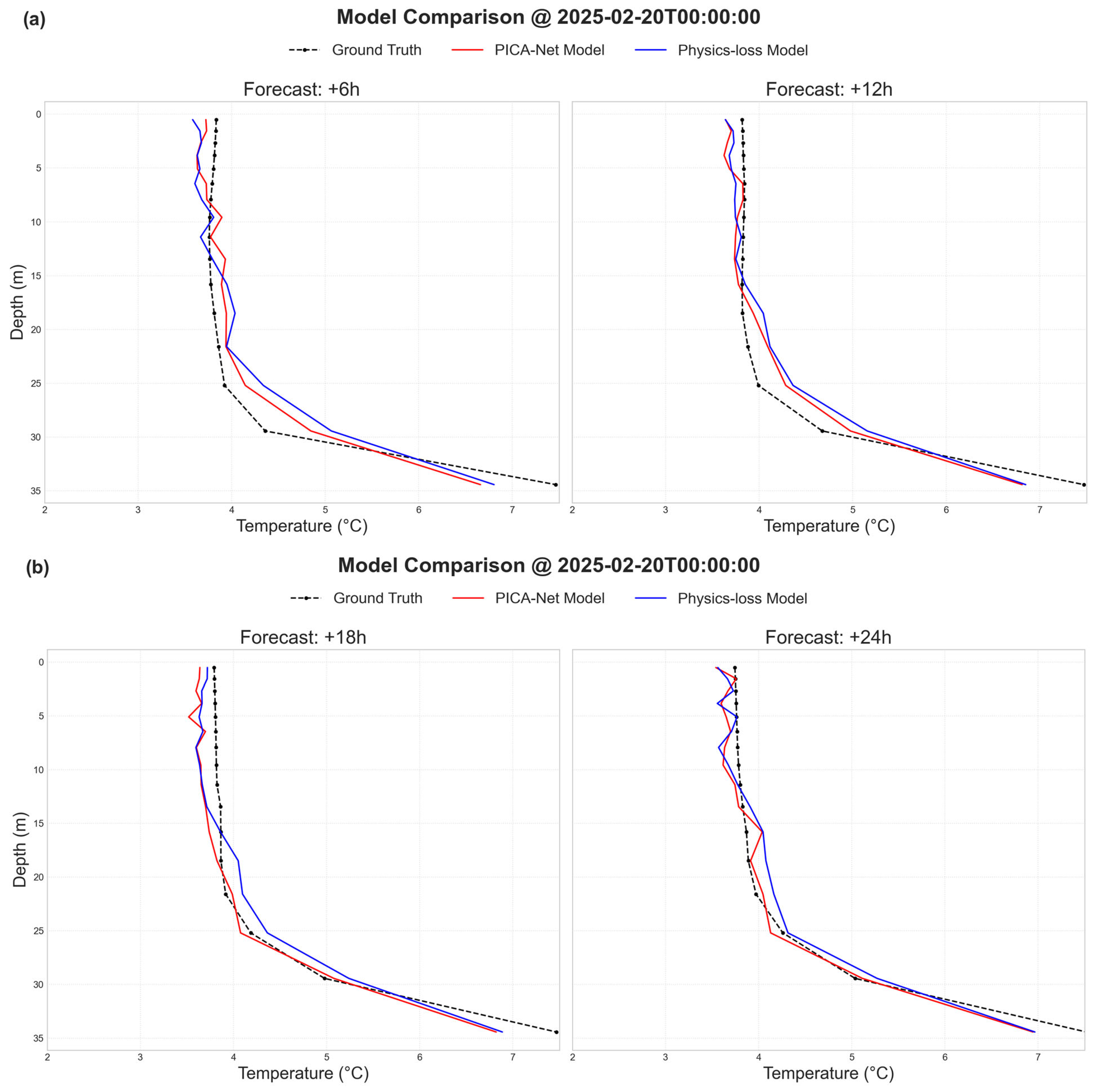
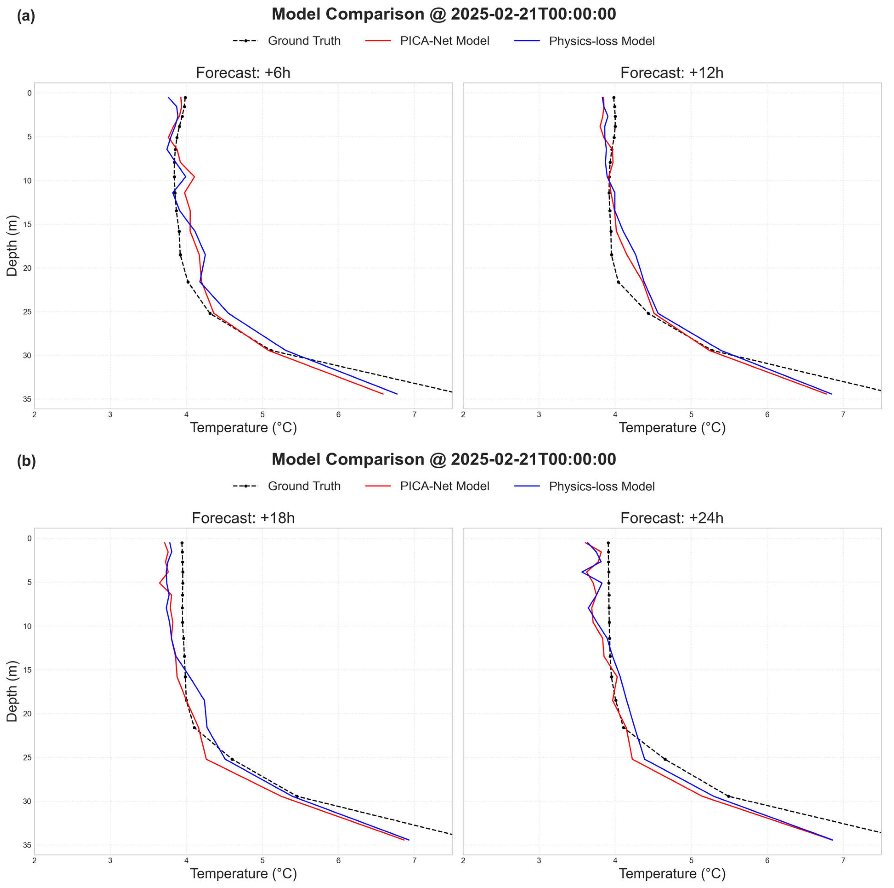
However, scalar metrics like RMSE may overlook structural improvements. To further evaluate model behavior, we performed case-by-case profile visualizations to examine whether physical constraints enhance the consistency and interpretability of predicted thermal structures under complex oceanic conditions.

In Figure 3 and Figure 4, we present the model’s prediction results over two consecutive days, 20–21 February 2025:

The black dashed line denotes the observed temperature profile (ground truth). The red solid line represents the prediction of the baseline PICA-Net model without physical constraints. The blue solid line shows the prediction from PICA-Net trained with physical constraints.

3.7. Edge Deployment Experiment

To evaluate the real-world deployment potential of the proposed temperature profile prediction model, a series of edge computing experiments were conducted, including model optimization, accuracy verification, and performance benchmarking. We tested on two platforms: a mainstream PC (Intel i7-10750H, RTX 1650Ti, Intel, Santa Clara, CA, USA) as baseline, and the NVIDIA Jetson TX2 as the target edge device (Nvidia, Santa Clara, CA, USA). The full hardware and software configurations are listed in

Table 6. Experimental platform hardware and software configuration table.

Platform	Components	Specifications/Versions
PC Platform	CPU	Intel(R) Core(TM) i7-10750H CPU @ 2.60 GHz 2.59 GHz
	GPU	NVIDIA GeForce RTX 1650ti
	RAM	16 GB
	Software Environment	Windows 11, Python 3.8, Pytorch 2.4.1, CUDA 11.8
Edge Computing Platform	CPU	NVIDIA Jetson TX2 (integrated quad-core ARM A57 and dual-core NVIDIA Denver 2)
	GPU	256-core NVIDIA Pascal™ architecture GPU
	RAM	8 GB LPDDR4
	Software Environment	NVIDIA JetPack 4.6.6, TensorRT 8.2.1.9, CUDA 10.2

.

The trained PyTorch model was first converted to ONNX format and then optimized using TensorRT to generate three inference engines: FP32 (baseline), FP16 (reduced precision for speed), and INT8 (quantized for maximum efficiency). To evaluate deployment effectiveness, we measured inference time, RMSE accuracy, power consumption, and model size across configurations. Results are summarized in

Table 7. Performance comparison of models on different platforms and optimization levels.

Model/Platform	Test Scope	Inference Time (ms)	RMSE (°C)	Power Consumption (mW)	Size (MB)
PC (CPU)	Full validation set	1.2467	~0.4	-	0.88
PC (GPU)	Full validation set	0.8876	~0.4	-	0.88
PC (GPU)	100 sample subsets	0.8876	0.250139	-	0.88
Jetson TX2 (FP32)	100 sample subsets	3.7240	0.250139	~3830	4.2
Jetson TX2 (FP16)	100 sample subsets	2.9758	0.250408	~4353	3.9
Jetson TX2 (INT8)	100 sample subsets	3.1735	0.250139	~4072	4.2

.

4. Discussion

This chapter analyzes the experimental results in depth, going beyond metric comparisons to explore physical mechanisms, model behavior, and scientific significance. It provides a comprehensive evaluation of PICA-Net, emphasizing its accuracy, physical consistency, generalization, and applicability to real-time ocean temperature profile forecasting.

4.1. Discussion on the Importance of Remote Sensing Features

Feature ablation experiments (Table 2) confirm that all evaluated satellite remote sensing variables significantly enhance PICA-Net’s prediction accuracy. Wind stress and wind speed had the greatest impact—removing them increased RMSE by 13.92% and 11.78%, respectively—highlighting the dominant role of wind-driven mixing in shaping short-term temperature structure. Similar conclusions on the influence of wind-stress on surface temperature and mixing have been reached in studies leveraging satellite wind products and flux retrievals [29]. Sea surface height anomaly (ZOS), when removed, led to a 9.70% RMSE rise, underscoring its value in capturing subsurface dynamics like eddies and fronts. SST and net heat flux (Q_net) contribute to surface thermal processes; removing them caused a 7.02% performance drop [30,31]. When all remote sensing features were excluded, RMSE rose by 13.01%, showing that PICA-Net benefits from the synergy of diverse physical variables. Overall, the results validate the model’s multi-source input design and emphasize the importance of integrating dynamic and thermodynamic satellite data for accurate regional rapid forecasting of ocean temperature profiles.

4.2. Analysis of Synergistic Effects in Model Architecture

Module ablation experiments (Table 3) reveal that PICA-Net’s high accuracy stems from the collaborative function of its three core components—1D-CNN, Bi-LSTM, and attention—rather than reliance on any single module. Removing the 1D-CNN led to the largest performance degradation, with RMSE increasing by 28.70%, confirming its role in extracting spatial patterns like thermoclines and mixed layers. Eliminating Bi-LSTM resulted in a 13.48% increase in RMSE, highlighting its importance for modeling temporal dependencies in dynamic ocean processes. Although removing the attention mechanism caused the smallest impact (RMSE increased by 4.81%), it significantly improves the model’s adaptability by dynamically reweighting features under varying conditions such as storms or calm periods. These findings confirm the architectural synergy of PICA-Net, where each module contributes uniquely to building a compact, accurate, and physically consistent prediction system [32].

4.3. Performance Comparison of PICA-Net with Other Models

To validate the performance of PICA-Net, we compared it with several representative baseline models. Among deep learning approaches, the Temporal Convolutional Network (TCN) achieved the lowest MAE (0.2842 °C), slightly outperforming PICA-Net (0.2876 °C). However, PICA-Net demonstrated superior RMSE (0.4073 °C vs. 0.4187 °C), indicating better robustness against large deviations—crucial for real-world applications [33]. LSTM and Transformer models performed worse, with RMSEs 6.31% and 8.30% higher than PICA-Net, respectively, underscoring the importance of combining temporal and spatial feature extraction [34]. In contrast, the Random Forest model exhibited the poorest performance (RMSE 0.7681 °C), revealing its limitations in modeling complex spatiotemporal ocean dynamics. These results collectively confirm that PICA-Net achieves state-of-the-art accuracy, physical reliability, and generalization capacity for temperature profile prediction.

4.4. Analysis of Model Prediction Error

4.4.1. Error Analysis for Different Forecast Lead Times

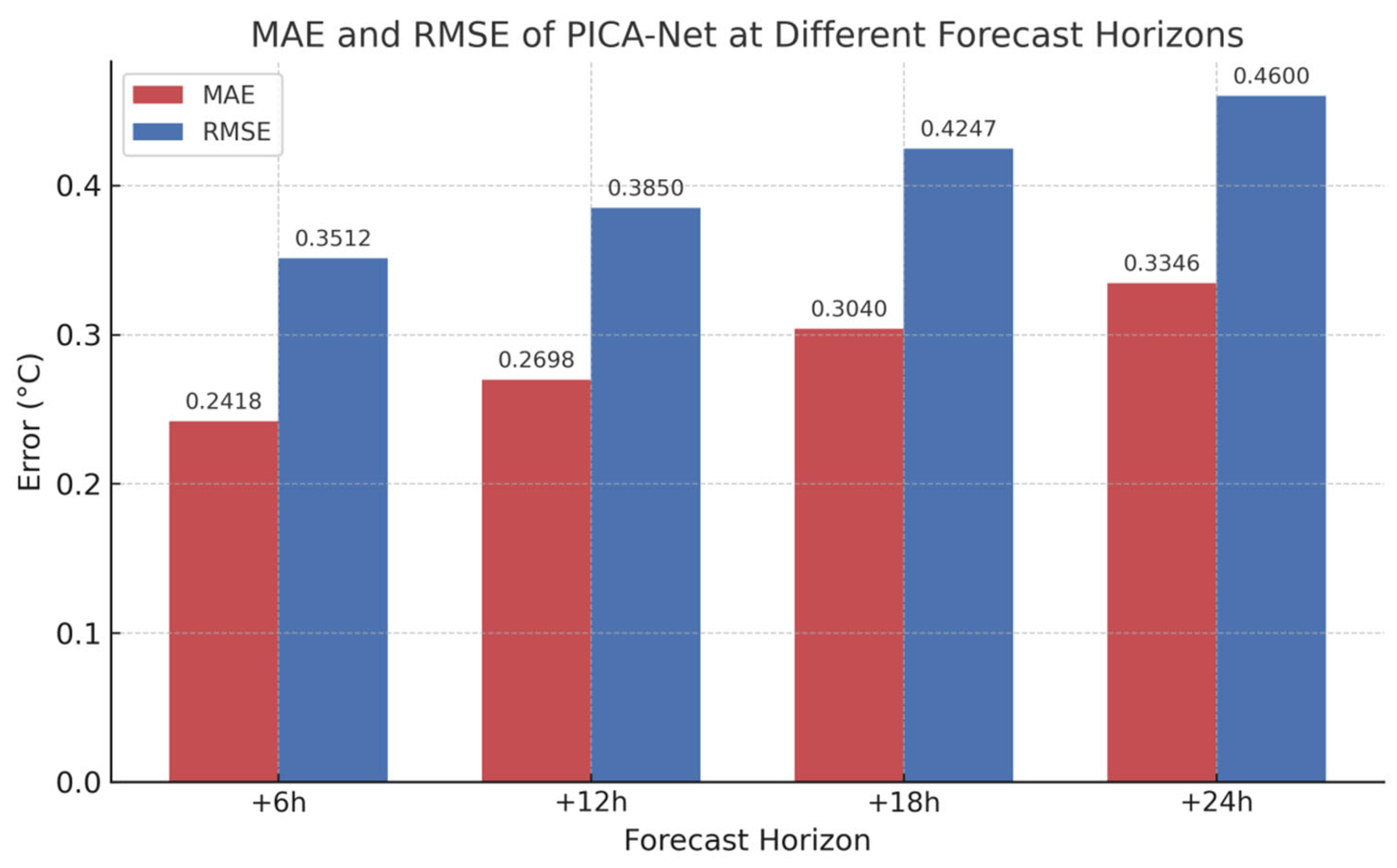
To assess short-term forecast stability, we evaluated PICA-Net’s performance at 6, 12, 18, and 24 h lead times. The experimental results are shown in Figure 5, clearly revealing the pattern of how the model’s error increases with the forecast lead time.

As shown in Figure 5, both MAE and RMSE increase steadily with longer horizons—RMSE rising from 0.3512 °C at +6 h to 0.4600 °C at +24 h, a 30% increase. This reflects typical prediction error accumulation and reduced ocean predictability at longer scales due to random, high-frequency dynamics. Nevertheless, PICA-Net consistently maintained high accuracy (overall RMSE = 0.4073 °C), demonstrating robust short-term forecasting capability.

4.4.2. Vertical Distribution Characteristics of Prediction Errors

To further investigate the ability of the PICA-Net model to reproduce the vertical structure of the ocean, we calculated the average prediction error (MAE and RMSE) of the model across the entire validation set and at each standard depth layer. The results are shown in Figure 6, where the red solid line represents MAE and the blue solid line represents RMSE.

Results show low errors in the upper ocean (0–18 m), where the model benefits from surface remote sensing inputs like SST, Q_net, and wind fields. However, errors increase sharply below the thermocline (~18 m), peaking at 34.4 m (MAE ≈ 0.5 °C, RMSE ≈ 0.7 °C). This trend reflects the model’s limited ability to infer deep-layer dynamics using only surface data. The continued error growth at depth highlights the challenge of predicting subsurface thermal structures without direct physical constraints, especially as internal oceanic processes dominate. Future improvements may require incorporating indirect subsurface indicators or assimilating sparse in situ profile data.

4.5. Further Discussion on the Regularization Effect of Physical Constraints

Although the introduction of physical constraints slightly increased RMSE, qualitative results (Figure 3 and Figure 4) show that these terms effectively regularize the model by suppressing nonphysical spikes and high-frequency jitters. While baseline predictions may align numerically with ground truth, they often violate fluid thermodynamic principles. Predictions from PICA-Net trained with physical constraints yield smoother, physically plausible profiles, improving interpretability and stability. This highlights the importance of integrating physical priors into neural networks, demonstrating the synergy between data-driven learning and physical laws in enhancing ocean prediction quality [35].

4.6. Discussion of Edge Deployment Experiments

4.6.1. Accuracy Validation Analysis

As shown in Table 7, the proposed model achieved a baseline RMSE of ~0.4 °C on the full validation set. To assess the impact of deployment and quantization, 100 samples were tested across platforms. On PC (GPU), the model yielded an RMSE of 0.250139 °C; the same value was obtained on Jetson TX2 using the FP32 engine, confirming that the PyTorch → ONNX → TensorRT pipeline is accurate and lossless. Quantized versions showed minimal to zero precision loss: the FP16 engine had only a 0.1% increase in RMSE, and the INT8 version maintained identical accuracy. These results validate the model’s suitability for efficient edge deployment without sacrificing prediction accuracy.

4.6.2. Real-Time Performance and Resource Consumption Analysis

Real-time inference is essential for operational forecasting. On Jetson TX2, the model achieves an inference time of 3.72 ms with FP32, which is further reduced to 2.98 ms after FP16 quantization—improving speed by 25% without loss of accuracy. Although the TensorRT engine file (~4 MB) is larger than the original PyTorch weights (~0.88 MB), this increase is justified by the engine’s precompiled optimizations and remains negligible relative to edge device storage capacity. Slightly higher instantaneous power consumption in FP16 and INT8 modes results from denser computations per unit time, but shorter inference durations keep total energy use low. Overall, the FP16-optimized model offers a balanced solution, combining fast inference, high accuracy, and efficient resource usage, making it well-suited for edge-based, regional rapid forecasting of ocean temperature profiles.

4.7. Limitations

While PICA-Net demonstrates promising performance in short-term temperature profile forecasting, several limitations remain. First, the current model is trained entirely on reanalysis products, which, while already assimilating a wide range of in situ and satellite observations, still represent a single class of processed data. This limits the diversity of input data sources, and future work will explore the integration of additional real-time observations to further enhance model robustness. Second, although physically inspired loss terms are incorporated, they are relatively simple and do not fully represent three-dimensional dynamics, internal waves, or nonlinear oceanic processes. Third, the model’s predictive skill decreases with depth, reflecting the challenge of inferring deep-layer thermal structures primarily from surface and near-surface inputs. Lastly, this study focuses solely on temperature prediction; extending the framework to salinity, currents, or biogeochemical variables remains unexplored. These limitations will be addressed in future iterations of the system.

5. Conclusions

This paper presents and systematically validates a lightweight deep learning framework, PICA-Net, designed to provide hourly resolution temperature profile forecasts with edge deployment capabilities for practical applications such as smart fisheries, marine environmental monitoring and regional rapid forecasting. By integrating multi-source physical driving features—particularly key satellite remote sensing variables—the model effectively captures the dominant dynamic mechanisms governing vertical thermal evolution in the ocean.

Architecturally, PICA-Net aims to jointly model local vertical structures, temporal evolution, and feature importance. Experimental results demonstrate that, across a 24 h prediction horizon with 6 h intervals, PICA-Net consistently outperforms representative baseline models in terms of accuracy, physical consistency, and deployment efficiency, highlighting its potential for real-world operational use.

Furthermore, this study incorporates additional physical constraints into the model’s loss function, including thermal diffusion smoothing, mixed-layer depth (MLD) consistency, and net heat flux consistency. Although adding these physical constraints slightly increases the overall RMSE, they significantly improve the stability of predicted thermocline structures and suppress nonphysical anomalies in the temperature field. This demonstrates the feasibility and value of using weak physical regularization to improve the physical plausibility of data-driven predictions.

Despite strong performance in the upper and mid-depth layers, depth-wise error analysis indicates that PICA-Net’s performance in deeper layers still has room for improvement. Future work will explore the inclusion of richer sub-surface features to enhance the model’s ability to capture deep ocean thermal dynamics. In addition, we plan to integrate real-time observational data from in situ dissolved oxygen chain sensors and develop corresponding data assimilation mechanisms to improve the model’s real-time adaptability and robustness. This transition from reanalysis-based training to real-time in situ data integration will also enable the model to evolve into a truly field-operational forecasting system. Ultimately, we aim to build a high-resolution, physically consistent, and flexible temperature profile prediction system, enabling regional rapid forecasting and offering reliable technical support for smart fisheries, coastal ecological monitoring, and marine hazard early warning applications.

References

1. Carvalho, K.; Wang, S. Sea Surface Temperature Variability in the Arctic Ocean and Its Marginal Seas in a Changing Climate: Patterns and Mechanisms. Glob. Planet. Change 2020, 193, 103265. [Google Scholar] [CrossRef]
2. Merchant, C.J.; Harris, A.R. Thermal Remote Sensing of Sea Surface Temperature. In Thermal Infrared Remote Sensing: Sensors, Methods, Applications; Kuenzer, C., Dech, S., Eds.; Remote Sensing and Digital Image Processing; Springer: Dordrecht, The Netherlands, 2013; Volume 17, pp. 287–313. [Google Scholar] [CrossRef]
3. Stansfield, A.M.; Reed, K.A. Global Tropical Cyclone Precipitation Scaling with Sea Surface Temperature. NPJ Clim. Atmos. Sci. 2023, 6, 60. [Google Scholar] [CrossRef]
4. Cronin, M.F.; Toole, J.M.; Firing, E.; Keffer, B.; Chiu, T.; Gundersen, K.S. Upper-Ocean Vertical Structure and Mixing Processes. NOAA/Pacific Marine Environmental Laboratory Technical Memorandum OAR-PMEL-187 2000. Available online: https://www.pmel.noaa.gov/people/cronin/encycl/ms0149.pdf (accessed on 15 July 2025).
5. León-Mimila, P.; Masouleh, F.K.; Takan, Z.; Junta, M. A Review of Ocean/Sea Subsurface Water Temperature Studies and Their Implications for Fisheries Management. Water 2017, 9, 936. [Google Scholar] [CrossRef]
6. FAO. Impacts of Climate Change on Fisheries and Aquaculture; Food and Agriculture Organization of the United Nations: Rome, Italy, 2018. [Google Scholar]
7. Park, Y.; Jeon, C.; Song, H.; Choi, Y.; Chae, J.-Y.; Lee, E.-J.; Kim, J.S.; Park, J.-H. Novel Method for the Estimation of Vertical Temperature Profiles Using a Coastal Acoustic Tomography System. Front. Mar. Sci. 2021, 8, 675456. [Google Scholar] [CrossRef]
8. Kerry, C.; Roughan, M.; de Souza, J.M.A. Assessing the Impact of Subsurface Temperature Observations from Fishing Vessels on Temperature and Heat Content Estimates in Shelf Seas: A New Zealand Case Study Using Observing System Simulation Experiments. Front. Mar. Sci. 2024, 11, 1358193. [Google Scholar] [CrossRef]
9. Xia, C.; Guo, J.; Nie, L.Y.; Li, J.C.; Wu, H.; Zhang, W.C.; Tian, Y.J.; Liu, Y.; Sun, P.; Ye, Z.J.; et al. The Influence of Ocean Processes on Fine-Scale Changes in the Yellow Sea Cold Water Mass Boundary Area Structure Based on Acoustic Observations. Remote Sens. 2023, 15, 4272. [Google Scholar] [CrossRef]
10. Hu, Y.; Yu, F.; Si, G.; Sun, F.; Liu, X.; Diao, X.; Chen, Z.; Nan, F.; Ren, Q. The Seasonal Evolution of the Yellow Sea Cold Water Mass Circulation: Roles of Fronts, Thermoclines, and Tidal Rectification. Ocean Model. 2024, 190, 102375. [Google Scholar] [CrossRef]
11. Pereiro, D.; Belyaev, O.; Dunbar, M.B.; Conway, A.; Dabrowski, T.; Graves, I.; Navarro, G.; Nolan, G.; Pearlman, J.; Simpson, P.; et al. An observational and warning system for the aquaculture sector. Front. Mar. Sci. 2023, 10, 1288610. [Google Scholar] [CrossRef]
12. Chatziantoniou, A.; Papandroulakis, N.; Stavrakidis-Zachou, O.; Spondylidis, S.; Taskaris, S.; Topouzelis, K. Aquasafe: A remote sensing, web-based platform for the support of aquaculture monitoring and decision-making. Appl. Sci. 2023, 13, 6122. [Google Scholar] [CrossRef]
13. Reichl, B.G.; Adcroft, A.; Griffies, S.M.; Hallberg, R. A Potential Energy Analysis of Ocean Surface Mixed Layers. J. Geophys. Res. Oceans 2021, 126, e2021JC018140. [Google Scholar] [CrossRef]
14. Yu, X.; Li Yi, D.; Wang, P. Enhancing Ocean Temperature and Salinity Reconstruction with Deep Learning: The Role of Surface Waves. J. Mar. Sci. Eng. 2025, 13, 910. [Google Scholar] [CrossRef]
15. Adams, K.; MacKinnon, J.; Lucas, A.J.; Nash, J.; Shroyer, E.; Farrar, J.T. Multi-platform observations of small-scale lateral mixed layer variability in the northern Bay of Bengal. Deep Sea Res. Part II Top. Stud. Oceanogr. 2019, 168, 104629. [Google Scholar] [CrossRef]
16. Li, S.; Wang, J.; Liu, K.; Guo, W.; Da, L.; Liu, J.; Hu, H.; Cui, B. Improving the Thermal Structure Predictions in the Yellow Sea by Field-Targeted Observations. Sci. Rep. 2021, 11, 19518. [Google Scholar] [CrossRef]
17. Chih, C.-H.; Wu, C.-C. Exploratory Analysis of Upper-Ocean Heat Content and Sea Surface Temperature Underlying Tropical Cyclone Rapid Intensification in the Western North Pacific. J. Clim. 2019, 33, 1031–1050. [Google Scholar] [CrossRef]
18. Zhao, X.Y.; Qi, J.P.; Yu, Y.W.; Zhou, L. Deep Learning for Ocean Temperature Forecasting: A Survey. Intell. Mar. Technol. Syst. 2024, 2, 28. [Google Scholar] [CrossRef]
19. Ko, K.-S.; Kim, Y.-W.; Byeon, S.-H.; Lee, S.-J. LSTM-Based Prediction of Ocean Mixed-Layer Temperature Using Meteorological Data. Korean J. Remote Sens. 2021, 37, 603–614. [Google Scholar] [CrossRef]
20. Zhang, Q.; Wang, H.; Dong, J.; Zhong, G.; Sun, X. Prediction of Sea Surface Temperature using Long Short-Term Memory. IEEE Geosci. Remote Sens. Lett. 2017, 14, 757–761. [Google Scholar] [CrossRef]
21. Zhang, K.; Geng, X.; Yan, X.-H. Prediction of 3-D Ocean Temperature by Multilayer Convolutional LSTM. IEEE Geosci. Remote Sens. Lett. 2020, 17, 1303–1307. [Google Scholar] [CrossRef]
22. Zuo, X.; Zhou, X.; Guo, D.; Li, S.; Liu, S.; Xu, C. Ocean Temperature Prediction Based on Stereo Spatial-and-Temporal 4-D Convolution Model. IEEE Geosci. Remote Sens. Lett. 2021, 19, 1003405. [Google Scholar] [CrossRef]
23. Su, H.; Zhang, T.; Lin, M.; Lu, W.; Yan, X.-H. Predicting Subsurface Thermohaline Structure from Remote Sensing Data Based on Long Short-Term Memory Neural Networks. Remote Sens. Environ. 2021, 260, 112465. [Google Scholar] [CrossRef]
24. Yang, Y.; Lam, K.-M.; Dong, J.; Ju, Y. Multi-Factor Deep Learning Model for Sea Surface Temperature Forecasting. Remote Sens. 2025, 17, 752. [Google Scholar] [CrossRef]
25. Wang, J.; Li, J.; Wang, X.; Wang, T.; Sun, Q. An Air Quality Prediction Model Based on CNN-BiNLSTM-Attention. Environ. Dev. Sustain. 2022, 24, 8674–8689. [Google Scholar] [CrossRef]
26. Tekin, S.F.; Fazla, A.; Kozat, S.S. Numerical Weather Forecasting using Convolutional-LSTM with Attention and Context Matcher Mechanisms. arXiv 2021, arXiv:2102.00696. [Google Scholar]
27. Ouala, S.; Brunton, S.L.; Pascual, A.; Chapron, B.; Collard, F.; Gaultier, L.; Fablet, R. Bounded Nonlinear Forecasts of Partially Observed Geophysical Systems with Physics-Constrained Deep Learning. Phys. D Nonlinear Phenom. 2023, 446, 133630. [Google Scholar] [CrossRef]
28. Hersbach, H.; Bell, B.; Berrisford, P.; Hirahara, S.; Horányi, A.; Muñoz-Sabater, J.; Nicolas, J.; Peubey, C.; Radu, R.; Schepers, D.; et al. The ERA5 Global Reanalysis. Q. J. R. Meteorol. Soc. 2020, 146, 1999–2049. [Google Scholar] [CrossRef]
29. Bourassa, M.A.; Meissner, T.; Cerovecki, I.; Chang, P.S.; Dong, X.; De Chiara, G.; Donlon, C.; Dukhovskoy, D.S.; Elya, J.; Fore, A.; et al. Remotely Sensed Winds and Wind Stresses for Marine Forecasting and Ocean Modeling. Front. Mar. Sci. 2019, 6, 443. [Google Scholar] [CrossRef]
30. Li, J.-L.F.; Tsai, Y.-C.; Xu, K.-M.; Lee, W.-L.; Jiang, J.H.; Yu, J.-Y.; Fetzer, E.J.; Stephens, G. Inferring the linkage of sea surface height anomalies, surface wind stress and sea surface temperature with the falling ice radiative effects using satellite data and global climate models. Environ. Res. Commun. 2022, 4, 125004. [Google Scholar] [CrossRef]
31. Maloney, E.D.; Chelton, D.B. An Assessment of the Sea Surface Temperature Influence on Surface Wind Stress in Numerical Weather Prediction and Climate Models. J. Clim. 2006, 19, 2743–2762. [Google Scholar] [CrossRef]
32. Shi, B.; Ge, C.; Lin, H.; Xu, Y.; Tan, Q.; Peng, Y.; He, H. Sea Surface Temperature Prediction Using ConvLSTM-Based Model with Deformable Attention. Remote Sens. 2024, 16, 4126. [Google Scholar] [CrossRef]
33. Yan, J.; Mu, L.; Wang, L.; Ranjan, R.; Zomaya, A.Y. Temporal Convolutional Networks for the Advance Prediction of ENSO. Sci. Rep. 2020, 10, 8055. [Google Scholar] [CrossRef] [PubMed]
34. Zhang, T.; Lin, P.; Liu, H.; Wang, P.; Wang, Y.; Zheng, W.; Yu, Z.; Jiang, J.; Li, Y.; He, H. A New Transformer Network for Short-Term Global Sea Surface Temperature Forecasting: Importance of Eddies. Remote Sens. 2025, 17, 1507. [Google Scholar] [CrossRef]
35. Zhang, L.; Duan, W.; Cui, X.; Liu, Y.; Huang, L. Surface Current Prediction Based on a Physics-Informed Deep Learning Model. Appl. Ocean Res. 2024, 148, 104005. [Google Scholar] [CrossRef]
Figure 1. Study area. Red point “A” is our study area.
Applsci 15 09204 g001
Figure 2. PICA-Net architecture.
Applsci 15 09204 g002
Figure 3. Comparison of predicted temperature profiles from the PICA-Net model and the Physics-loss model against the ground truth on 20 February 2025. The ground truth (black dashed line) is plotted alongside predictions from PICA-Net (red line) and the Physics-loss model (blue line). The sub-figures show the predicted profiles for different forecast horizons: (a) +6 h and +12 h, and (b) +18 h and +24 h.
Applsci 15 09204 g003
Figure 4. Comparison of predicted temperature profiles from the PICA-Net model and the Physics-loss model against the ground truth on 21 February 2025. The ground truth (black dashed line) is plotted alongside predictions from PICA-Net (red line) and the Physics-loss model (blue line). The sub-figures show the predicted profiles for different forecast horizons: (a) +6 h and +12 h, and (b) +18 h and +24 h.
Applsci 15 09204 g004
Figure 5. MAE and RMSE of PICA-Net at different forecast horizons.
Applsci 15 09204 g005
Figure 6. MAE and RMSE of PICA-Net at different ocean depths.
Applsci 15 09204 g006