Article

Model Comparison and Parameter Estimation for Gompertz Distributions Under Constant Stress Accelerated Lifetime Tests

School of Mathematics and Statistics, Beijing Jiaotong University, Beijing 100044, China
*
Author to whom correspondence should be addressed.
Appl. Sci. 2025, 15(16), 9199; https://doi.org/10.3390/app15169199
Submission received: 21 July 2025 / Revised: 16 August 2025 / Accepted: 19 August 2025 / Published: 21 August 2025

Abstract

The accelerated lifetime test is a widely used and effective approach in reliability analysis because of its shorter testing duration. In this study, product lifetimes are assumed to follow the Gompertz distribution. This article primarily focuses on performance comparisons between the linear model and the inverse power-law model, both of which are utilized to characterize the relationship between the shape parameter and stress levels. To test model robustness, we also generate data from the Sine-Modified Power Gompertz distribution, a more flexible alternative. We conduct Monte Carlo simulations using four estimation methods: the maximum likelihood method, the least squares method, the maximum product of spacing method, and the Cramér-von Mises method, for small, medium, and large sample sizes. The comparison of mean squared error serves as a critical indicator for evaluating the performance of different methods and models. Additionally, the shape parameter and reliability function are obtained based on the estimation results. Finally, a real dataset is analyzed to demonstrate the most suitable accelerated life model, and the Akaike Information Criterion is used to further assess model fit. Furthermore, we employ leave-one-out cross-validation (LOOCV) to prove this model’s generalizability.

1. Introduction

Reliability studies have gained paramount importance in diverse industrial sectors, including electronics, automotive systems, and automation technologies. Despite its significance, traditional reliability testing often incurs prohibitive costs due to the lengthy durations required to observe failure times under normal operating conditions. For high-reliability products, such as aerospace components or medical devices, failure events may manifest only after years or decades of service, which makes the traditional testing method unfeasible. To address this problem, the accelerated lifetime test (ALT) was introduced by Nelson [1], revolutionizing reliability experimentation. By subjecting test units to elevated stress levels—such as increased temperature, voltage, or mechanical load—the ALT accelerates failure mechanisms while maintaining failure mode consistency with normal conditions. This approach enables the extrapolation of lifetime characteristics through mathematical modeling of stress-life relationships, significantly reducing both testing time and cost. Accelerated lifetime modeling has been systematically advanced by Meeker [2] (statistical frameworks for ALT data), Limon [3] (adaptive stress test design), and Bagdonavicius [4] (parametric models for degradation processes). In this approach, we establish the test conditions at elevated levels, such as increased current, voltage, temperature, or humidity, to accelerate the lifetime testing of units. There are various methods for designing stress in accelerated lifetime test, including constant stress, step stress [5], ramp stress [6], and others. Furthermore, a combination of these methods can be utilized in experiments. However, the constant stress accelerated lifetime test (CSALT) is the most commonly used approach in studies, as it allows for the collection of more accurate and reliable data through a simpler testing process. We can learn more about the optimal constant-stress accelerated life test framework from Ling [7]. Furthermore, many researchers have explored the CSALT using various distributions. For instance, Mazen Nassar [8] investigated the exponentiated Rayleigh distribution under the CSALT, while Devendra Kumar [9] studied the CSALT based on the generalized inverse Lindley distribution.
In this article, we study the Gompertz distribution, first proposed by Gompertz [10]. It is widely used in survival analysis, actuarial science, and demography to model processes where failure rates increase with time. Many researchers have explored the properties of the Gompertz distribution, including Winsor [11] and Pollard [12].
This distribution is notable for its ability to model the increase in human mortality with age, as well as the aging-related failures of equipment or systems over time. These characteristics underpin its broad applicability in reliability studies. The Gompertz distribution has long been a cornerstone in reliability and survival analysis, prized for its ability to model failure rates that increase exponentially over time. However, real-world engineering systems and life data often exhibit more complex failure behaviors that cannot be adequately captured by the monotonic hazard rate of the classical Gompertz model. Recent statistical literature has focused on developing new families of distributions through generator functions. These generators transform a baseline distribution to create richer, more flexible models, often by introducing additional shape parameters. In this study, we adopt the recently proposed Sine-Modified Power-Generated family [13] to extend the Gompertz distribution. This approach combines the desirable properties of trigonometric functions with a power modification, aiming to create a highly adaptable model for accelerated life testing scenarios. This extension allows for a more rigorous evaluation of our proposed models, effectively testing their robustness and generalization capability against a significantly more flexible distributional framework. The standard Gompertz distribution is inherently constrained by its monotonically increasing hazard rate function, rendering it inadequate for capturing complex failure phenomena such as the bathtub-shaped or unimodal hazard rates characteristic of certain real-world engineering systems. Through the inclusion of an additional parameter, the SMPoG distribution achieves superior flexibility. This enables it to accommodate a wider spectrum of hazard rate patterns—encompassing increasing, decreasing, bathtub, and unimodal trends—making it a more powerful and applicable tool for modeling complex data from accelerated life tests.
This article focuses on statistical inference and establishes several objectives. Firstly, we aim to select an appropriate relationship between stress levels and the shape parameter in the Gompertz distribution. To accomplish this, we employ four estimation methods: maximum likelihood estimation (MLE), least squares estimation (LSE), maximum product spacing estimation (MPSE), and Cramér-von-Mises estimation (CVM). The performance of two models under these estimation methods is compared using their mean squared errors (MSEs), as discussed by Allen [14]. The foundations and methodologies of MLE, LSE, MPSE, and CVM have been explored extensively in works by Zhang and Wang [15], Fan and Yu [16], Abdel Ghaly [17], and Dey and Nassar [18,19], among others. Additionally, we conduct Monte Carlo simulations across different sample sizes—small, medium, and large—to assess the models’ performance under varying conditions. At the same time, quantitative comparison of parameter estimation methods can be studied from the results of Monte Carlo simulations. Insights into Monte Carlo simulation methodology can be found in Harrison [20]. Secondly, based on the estimations obtained in the first objective, we calculate the shape parameter and reliability function for the two models. This allows us to further evaluate the performance of the models and assess the accuracy of applying high-level estimators to standard conditions. Lastly, we use a real dataset to illustrate the advantages of the better-fitting Gompertz distribution model, highlighting its practical application and reliability in real scenarios.
The structure of this article is organized as follows. In Section 2, we discuss the fundamental properties of the Gompertz distribution and propose assumptions regarding the relationship between its shape parameter and stress levels. Section 3 focuses on deriving the objective functions for the four estimation methods—maximum likelihood estimation (MLE), least squares estimation (LSE), maximum product spacing estimation (MPSE), and Cramér-von-Mises estimation (CVM)—and we deduce the formulas for the shape parameter and the reliability function. Furthermore, we conduct three simulations focused on testing models’ robustness, by generating data from the Sine-Modified Power Gompertz (SMPoG) distribution. Section 4 presents the simulation study for two models under varying sample sizes. Additionally, we evaluate the performance of the shape parameter and reliability function under different scenarios. In Section 5, a real dataset is analyzed, where we calculate the Kolmogorov–Smirnov (K–S) distance and corresponding p-values, and additionally employ the Akaike Information Criterion (AIC) to evaluate the model’s performance on this dataset. Leave-one-out cross-validation (LOOCV) is further employed to rigorously evaluate the robustness and generalizability of the models. By iteratively holding out each sample as a validation set and training the model on the remaining data, this approach effectively leverages the limited dataset to assess how well the models perform on unseen data. To quantify predictive performance and intuitively distinguish the differences among estimation methods, we adopt three key metrics: mean absolute error (MAE) to measure average prediction bias, root mean squared error (RMSE) to emphasize larger deviations, and coefficient of variation (CV) to evaluate the stability of prediction errors. These metrics collectively provide a comprehensive view of both the accuracy and consistency of each method, reinforcing the reliability of our findings regarding model generalizability. Finally, in the concluding Section 6, we summarize our findings and discuss model selection based on the Gompertz distribution.

2. Model and Assumptions

2.1. The Basic Gompertz Distribution

The random variable T, assumed to represent the lifetime with value t, follows a Gompertz distribution. Its probability density function (pdf) is given as
f ( t ; η , b ) = η exp b t η b e b t 1 ; t > 0 , η , b > 0
The cumulative distribution function is
F ( t ; η , b ) = 1 exp η b e b t 1
The reliability function is
R ( t ; η , b ) = exp η b e b t 1
The hazard rate function is
h ( t ; η , b ) = η e b t
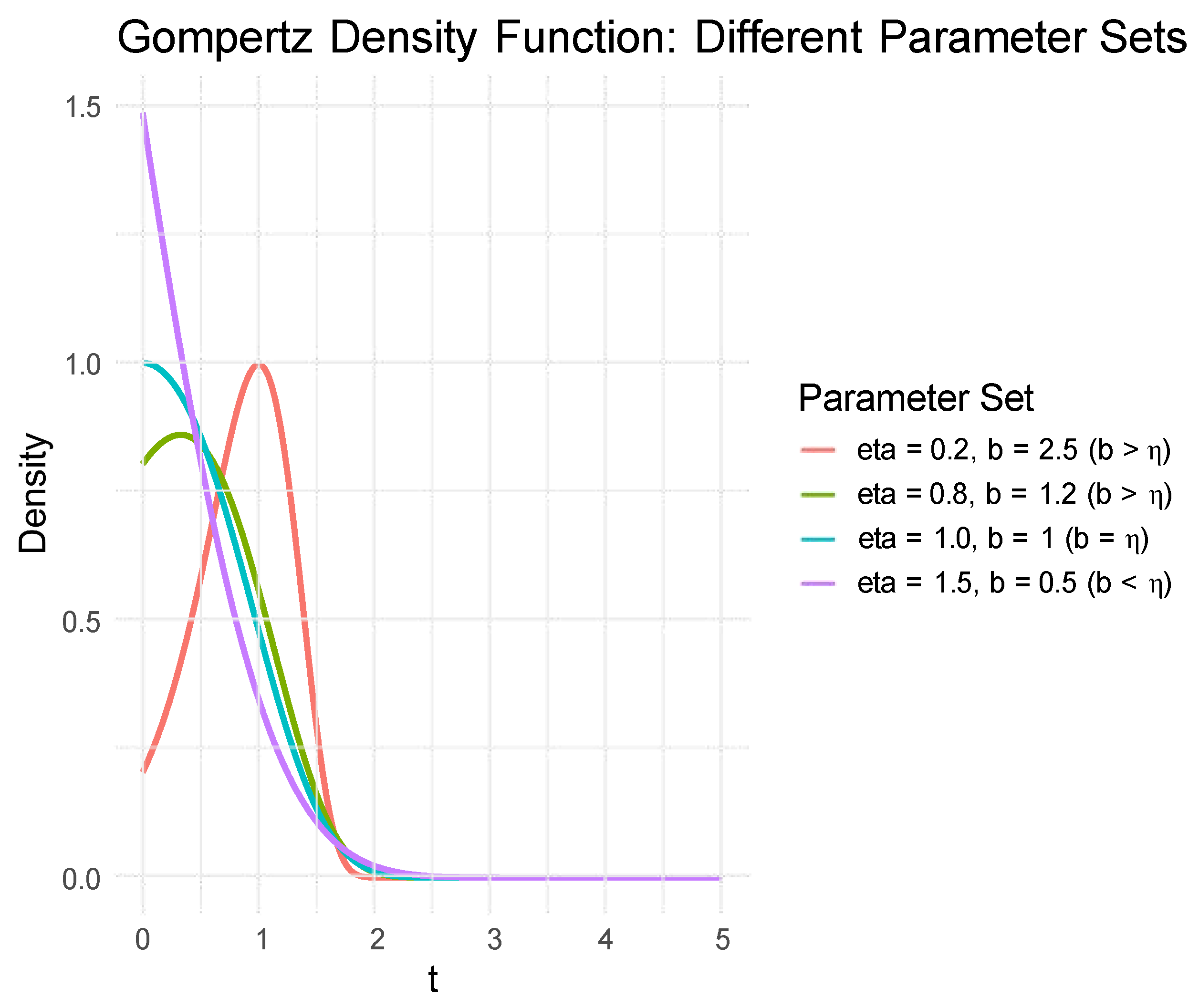
The shape of the Gompertz density function is jointly determined by the parameters η (the initial risk intensity) and b (the risk growth rate), and it exhibits two typical patterns, which can be seen in Figure 1. When b > η , the graph of the density function shows a unimodal and right-skewed distribution. It reaches its peak at the mode position t mode = 1 b ln b η and then decays at an exponential rate. When b < η , the density function displays a monotonically decreasing trend, reaching its maximum value at t = 0 , with f ( 0 ) = η . The density function continues to decrease as t increases, without exhibiting any local extrema.

2.2. The Sine-Modified Power Gompertz (SMPoG) Distribution

To enhance the flexibility of the classical Gompertz distribution, we introduce a more versatile framework by employing the Sine-Modified Power-Generated (SMPo-G) family, as proposed by Chesneau et al. (2023) [13]. This approach embeds the Gompertz distribution as the baseline, resulting in a new, more adaptable lifetime model, which we term the Sine-Modified Power Gompertz (SMPoG) distribution.
Let g ( t ; η , b ) and G ( t ; η , b ) be the probability density function (pdf) and cumulative distribution function (CDF) of the baseline Gompertz distribution, as given in Equations (1) and (2), respectively. The CDF of the general SMPo-G family is defined as:
F ( t ; α , η , b ) = sin π 2 G ( t ; η , b ) α G ( t ; η , b ) 1
where α > e 1 is an additional shape parameter that controls the degree of modification. The corresponding pdf is given by
f ( t ; α , η , b ) = π 2 g ( t ; η , b ) α G ( t ; η , b ) 1 1 + ln ( α ) G ( t ; η , b ) × cos π 2 G ( t ; η , b ) α G ( t ; η , b ) 1
By substituting the Gompertz CDF from (2) into (5), we obtain the explicit CDF of the new three-parameter SMPoG distribution:
F SMPoG ( t ; α , η , b ) = sin π 2 1 e η b ( e b t 1 ) α 1 e η b ( e b t 1 ) 1
The pdf, f SMPoG ( t ; α , η , b ) , is derived by substituting both the Gompertz CDF and pdf into (6). The resulting distribution is considerably more flexible than the standard Gompertz model.
The primary reliability functions for the SMPoG distribution can be derived as follows. The reliability (or survival) function, R ( t ) , is defined as R ( t ) = 1 F ( t ) . For the SMPoG distribution, it is:
R SMPoG ( t ; α , η , b ) = 1 F SMPoG ( t ; α , η , b )
where F SMPoG ( t ) is given by (7).
The hazard rate function (HRF), h ( t ) , which describes the instantaneous failure rate, is given by the ratio of the pdf to the reliability function:
h SMPoG ( t ; α , η , b ) = f SMPoG ( t ; α , η , b ) R SMPoG ( t ; α , η , b )
The inclusion of the parameter α allows the HRF to exhibit various shapes, including increasing, decreasing, and bathtub curves, which is a significant improvement over the monotonically increasing HRF of the standard Gompertz distribution.
The quantile function (QF), Q ( u ) = F 1 ( u ) for u ( 0 , 1 ) , is essential to generate random variates in Monte Carlo simulations. For the SMPoG family, the QF has a tractable form involving the Lambert W function. By inverting (5), we first solve for the baseline CDF value, G ( Q ( u ) ) :
G ( Q ( u ) ) = 1 ln ( α ) W 0 2 α ln ( α ) π arcsin ( u )
where W 0 ( · ) is the principal branch of the Lambert W function.
The quantile function of the baseline Gompertz distribution, G 1 ( u ; η , b ) , is found by inverting (2):
G 1 ( u ; η , b ) = 1 b ln 1 b η ln ( 1 u )
Finally, the quantile function of the SMPoG distribution is obtained by applying the Gompertz QF to the result from (10):
Q SMPoG ( u ; α , η , b ) = G 1 1 ln ( α ) W 0 2 α ln ( α ) π arcsin ( u ) ; η , b = 1 b ln 1 b η ln 1 1 ln ( α ) W 0 2 α ln ( α ) π arcsin ( u )

2.3. Constant Stress Accelerated Life Testing

The following assumptions are made for parameter estimation in constant stress accelerated life testing (CSALT) based on the Gompertz distribution:
  • There are totally N identical units, which are separated into K groups with sizes, n 1 , n 2 , …, n K , and j = 1 K n j = N .
  • There are K levels of accelerated stress, denoted as S j for j = 1 , 2 , , K , which are each applied to n j independent test units, where j = 1 , 2 , , K . Here, S 0 represents the normal stress condition, and the stress levels follow an increasing relationship:
    S 0 < S 1 < S 2 < < S K
  • There are two assumptions regarding the relationship between the scale parameter η and the constant stress S j :
    Assumption 1: Simple linear model (Model 1):
    η j = a + c S j
    Assumption 2: Inverse power-law model (Model 2):
    η j = a S j c
    where a and c are unknown parameters.
  • t i j represents the lifetime of the i-th unit under the j-th stress level.
  • The shape parameter η has direct relationship with stress level S j :
    In Model 1:
    η j = a + c S j
    In Model 2:
    η j = a S j c

3. Different Methods for Estimating Parameters in Two Models

In this section, four methods, including (1) the method of maximum likelihood, (2) the method of least squares, (3) the method of maximum product of spacing, and (4) the method of Cramér-von-Mises, are employed in parameter estimation under two different models. Sanku Dey’s study [21] provides a comprehensive investigation of estimation methodologies for the Gompertz distribution, offering valuable insight into parameter estimation method.

3.1. Maximum Likelihood Method

Maximum likelihood method is widely used in parameters’ estimation. Based on (1), we derive the joint maximum likelihood function as
M o d e l 1 : L 1 ( a , b , c d ) = j = 1 K i = 1 n j ( a + c S j ) · e b t i j · exp a + c S j b e b t i j 1
M o d e l 2 : L 2 ( a , b , c d ) = j = 1 K i = 1 n j a S j c · e b t i j · exp a S j c b e b t i j 1
where d represents { t i j } = { t i j j = 1 , 2 , , K ; i = 1 , 2 , , n j }
The log-likelihood function, denoted by ( a , b , c ) , is the natural logarithm of the likelihood function L ( a , b , c d ) :
( a , b , c ) = ln L ( a , b , c d ) .
M o d e l 1 : l 1 ( a , b , c ) = j = 1 K n j ln ( a + c S j ) + b j = 1 K i = 1 n j t i j 1 b j = 1 K ( a + c S j ) i = 1 n j e b t i j 1
M o d e l 2 : l 2 ( a , b , c ) = N ln a + c j = 1 K n j ln S j + b j = 1 K i = 1 n j t i j 1 b j = 1 K a S j c i = 1 n j e b t i j 1
We can obtain the MLEs (results estimated by maximum likelihood method) of a, b, c in Model 1 by solving the following equations.
l 1 a = N b + j = 1 K n j a + b S j j = 1 K i = 1 n j e b t i j b = 0 , l 1 b = a N b 2 j = 1 K n j c S j b 2 + j = 1 K n j S j a + b S j + j = 1 K i = 1 n j t i j e b t i j · t i j ( a + c S j ) b + e b t i j · a + c S j b 2 = 0 , l 1 c = j = 1 K n j S j b j = 1 K i = 1 n j e b t i j S j b = 0 .
MLEs of a, b, c in Model 2 can be obtained by solving the following equations.
l 2 a = N a + j = 1 K n j S j c b j = 1 K i = 1 n j e b t i j S j c b = 0 , l 2 b = j = 1 K n j a S j c b 2 + j = 1 K i = 1 n j t i j e b t i j t i j a S j c b + e b t i j a S j c b 2 = 0 , l 2 c = j = 1 K n j ln S j + j = 1 K n j a S j c ln S j b j = 1 K i = 1 n j e b t i j a S j c ln S j b = 0 .
However, since the above equations do not have closed-form solutions, numerical techniques are required to address these problems.

3.2. Method of Least Squares

The goal of the least squares method is to minimize the sum of the squared differences between the model’s predicted values and the actual observed data points. Within the framework of accelerated life tests under the Gompertz distribution, the empirical distribution function is approximated using the estimator i n j + 1 , which represents the cumulative proportion of failures observed at the i-th ordered failure time under the j-th stress level. This approximation is widely adopted in statistical inference for right-censored lifetime data analysis, providing a consistent and asymptotically efficient estimator of the underlying distribution function. The estimations can be obtained by minimizing the following formulas:
M o d e l 1 : S 1 ( a , b , c | d ) = j = 1 K i = 1 n j exp a + c S j b e b t i j 1 1 i n j + 1 2
M o d e l 2 : S 2 ( a , b , c | d ) = j = 1 K i = 1 n j exp a S j c b e b t i j 1 1 i n j + 1 2
The LSEs (results estimated by method of least squares) under Model 1 can be obtained by solving the following three nonlinear equations:
S 1 ( a , b , c ) a = j = 1 k i = 1 n j exp a + c S j b ( e b t i j 1 ) 1 i n j + 1 ψ 1 ( i j ) = 0 ,
S 1 ( a , b , c ) b = j = 1 k i = 1 n j exp a + c S j b ( e b t i j 1 ) 1 i n j + 1 ψ 2 ( i j ) = 0 ,
S 1 ( a , b , c ) c = j = 1 k i = 1 n j exp a + c S j b ( e b t i j 1 ) 1 i n j + 1 ψ 3 ( i j ) = 0 ,
where
ψ 1 ( i j ) = 1 b ( e b t i j 1 ) exp a + c S j b ( e b t i j 1 )
ψ 2 ( i j ) = exp a + c S j b ( e b t i j 1 ) · ( a + c S j ) ( e b t i j 1 ) b 2 t i j ( a + c S j ) e b t i j
ψ 3 ( i j ) = S j b ( e b t i j 1 ) exp a + c S j b ( e b t i j 1 )
The LSEs under Model 2 can be obtained by solving the following three nonlinear equations:
S 2 ( a , b , c , t ) a = 2 j = 1 K i = 1 n j exp a S j c b e b t i j 1 1 i n j + 1 · ξ 1 ( i j ) = 0 ,
S 2 ( a , b , c , t ) b = 2 j = 1 K i = 1 n j exp a S j c b e b t i j 1 1 i n j + 1 · ξ 2 ( i j ) = 0 ,
S 2 ( a , b , c , t ) c = 2 j = 1 K i = 1 n j exp a S j c b e b t i j 1 1 i n j + 1 · ξ 3 ( i j ) = 0 ,
where
ξ 1 ( i j ) = S j c b e b t i j 1 exp a S j c b e b t i j 1
ξ 2 ( i j ) = exp a S j c b e b t i j 1 · a S j c e b t i j 1 b 2 t i j a S j c e b t i j
ξ 3 ( i j ) = a S j c ln ( S j ) b e b t i j 1 exp a S j c b e b t i j 1
All of the above equations do not have closed-form solutions. We need to learn a numerical technique from Gill [22], who studied algorithms for solving linear least-squares problems.

3.3. Method of Maximum Product of Spacings

The maximum product of spacings estimates parameters by maximizing the geometric mean of uniform spacings, defined as the differences between consecutive cumulative distribution function (CDF) values of ordered data. For a random sample t 1 , t 2 , , t n , let t ( 1 ) t ( 2 ) t ( n ) denote the order statistics. The spacings are computed as
D i = F ( t ( i ) ) F ( t ( i 1 ) ) , i = 1 , 2 , , n + 1 ,
where F ( · ) is the theoretical CDF, t ( 0 ) = 0 , and t ( n + 1 ) = . In the end, we need to maximize i = 1 n + 1 D i . For the j-th stress group ( j = 1 , 2 , , K ), let t ( 1 ) j t ( 2 ) j t ( n j ) j denote the order statistics of the observed lifetimes { t 1 j , t 2 j , , t n j j } . These ordered data facilitate the computation of spacings.
D i j = F ( t ( i ) j ) F ( t ( i 1 ) j ) , i = 1 , 2 , , n j + 1 ,
which is used in the method of maximum product of spacings to estimate parameters across stress levels.
The cumulative function for two models are as follows:
M o d e l 1 : F 1 t i j ; η , b = 1 exp a + c S j b e b t i j 1
M o d e l 2 : F 2 t i j ; η , b = 1 exp a S j c b e b t i j 1
Furthermore, we derive D 1 i j ( D i j calculated in Model 1) and D 2 i j ( D i j calculated in Model 2):
D 1 , i j ( t i j a , b , c ) = F 1 ( t i j a , b , c ) F 1 ( t ( i 1 ) , j a , b , c )
D 2 , i j ( t i j a , b , c ) = F 2 ( t i j a , b , c ) F 2 ( t ( i 1 ) , j a , b , c )
The final objective formulas, which are expressed as M 1 ( a , b , c ) and M 2 ( a , b , c ) , are derived as follows:
M 1 ( a , b , c ) = j = 1 K i = 1 n j + 1 1 n j + 1 ln D 1 , i , j ( t i , j a , b , c )
M 2 ( a , b , c ) = j = 1 K i = 1 n j + 1 1 n j + 1 ln D 2 , i , j ( t i , j a , b , c )
The MPSEs (results estimated by method of maximum product of spacings) under Model 1 can be obtained by solving the following equations:
M 1 ( a , b , c ) a = j = 1 k i = 1 n j + 1 1 ( n j + 1 ) D i j ( a , b , c ) × ψ 1 ( i j ) ψ 1 ( i 1 ) j = 0 ,
M 1 ( a , b , c ) b = j = 1 k i = 1 n j + 1 1 ( n j + 1 ) D i j ( a , b , c ) × ψ 2 ( i j ) ψ 2 ( i 1 ) j = 0 ,
M 1 ( a , b , c ) c = j = 1 k i = 1 n j + 1 1 ( n j + 1 ) D i j ( a , b , c ) × ψ 3 ( i j ) ψ 3 ( i 1 ) j = 0 ,
The MPSEs under Model 2 can be obtained by solving the following equations:
M 2 ( a , b , c ) a = j = 1 k i = 1 n j + 1 1 ( n j + 1 ) D i j ( a , b , c ) × ξ 1 ( i j ) ξ 1 ( i 1 ) j = 0 ,
M 2 ( a , b , c ) b = j = 1 k i = 1 n j + 1 1 ( n j + 1 ) D i j ( a , b , c ) × ξ 2 ( i j ) ξ 2 ( i 1 ) j = 0 ,
M 2 ( a , b , c ) c = j = 1 k i = 1 n j + 1 1 ( n j + 1 ) D i j ( a , b , c ) × ξ 3 ( i j ) ξ 3 ( i 1 ) j = 0 ,
where ψ 1 ( i j ) , ψ 2 ( i j ) , ψ 3 ( i j ) , ξ 1 ( i j ) , ξ 2 ( i j ) , ξ 3 ( i j ) have been defined as (23)–(28).

3.4. Method of Cramér-Von Mises

The Cramér–von Mises criterion is a minimum-distance estimation approach, which minimizes the difference between the observed empirical distribution and the theoretical distribution. The feasibility of this method has been demonstrated by Macdonald [23]. The Cramér–von Mises estimators (CVMs) are obtained by minimizing the following objective function:
W 2 = [ F n ( x ) F ( x ; θ ) ] 2 d F ( x ; θ ) ,
where F n ( x ) is the empirical distribution function and F ( x ; θ ) is the theoretical cumulative distribution function parameterized by θ .
Based on the aforementioned theories, the objective function to be minimized can be expressed as follows:
M o d e l 1 : C 1 ( a , b , c | d ) = 1 12 N j = 1 K i = 1 n j ( ( F 1 ( t i j ) 2 i 1 2 n j ) ) 2
M o d e l 2 : C 2 ( a , b , c | d ) = 1 12 N j = 1 K i = 1 n j ( ( F 2 ( t i j ) 2 i 1 2 n j ) ) 2
CVMs (results estimated by method of Cramér-Von Mises) under Model 1 can be obtained by solving the following equations:
C 1 ( a , b , c | d ) a = 1 12 N j = 1 K i = 1 n j 2 1 exp a + c S j b ( e b t i j 1 ) 2 i 1 2 n j · ψ 1 ( i j ) = 0
C 1 ( a , b , c | d ) b = 1 12 N j = 1 K i = 1 n j 2 1 exp a + c S j b ( e b t i j 1 ) 2 i 1 2 n j · ψ 2 ( i j ) = 0
C 1 ( a , b , c | d ) c = 1 12 N j = 1 K i = 1 n j 2 1 exp a + c S j b ( e b t i j 1 ) 2 i 1 2 n j · ψ 3 ( i j ) = 0
CVMs under Model 2 can be obtained by solving the following equations:
C 2 ( a , b , c | d ) a = 1 12 N j = 1 K i = 1 n j 2 1 exp a S j c b ( e b t i j 1 ) 2 i 1 2 n j · ξ 1 ( i j ) = 0
C 2 ( a , b , c | d ) b = 1 12 N j = 1 K i = 1 n j 2 1 exp a S j c b ( e b t i j 1 ) 2 i 1 2 n j · ξ 2 ( i j ) = 0
C 2 ( a , b , c | d ) c = 1 12 N j = 1 K i = 1 n j 2 1 exp a S j c b ( e b t i j 1 ) 2 i 1 2 n j · ξ 3 ( i j ) = 0
where ψ 1 ( i j ) , ψ 2 ( i j ) , ψ 3 ( i j ) , ξ 1 ( i j ) , ξ 2 ( i j ) , ξ 3 ( i j ) have been defined as (23)–(28).

3.5. Inference on Shape Parameter and Reliability Prediction

Finally, the estimators of η j for the two models are derived from the MLEs, LSEs, MPSEs, and CVMs of parameters a and c, where η j follows the stress-lifetime relationship in Gompertz:
M o d e l 1 : η ^ j = a ^ + c ^ S j
M o d e l 2 : η ^ j = a ^ S j c ^
where a ^ and c ^ represent the estimates of the parameters a and b, obtained through the various estimation methods discussed earlier.
Under normal stress level S u , we can obtain the shape parameter from the following formulas:
M o d e l 1 : η ^ u = a ^ + c ^ S u
M o d e l 2 : η ^ u = a ^ S u c ^
Furthermore, the reliability under usual condition S u at the lifetime t 0 can be predicted by
R ^ u ( t 0 ) = exp η ^ u b ^ e b ^ t 0 1

3.6. Estimation for SMPoG Distribution via Grid Search

To enhance modeling flexibility, we now consider the case where the lifetime data follow the proposed SMPoG distribution. The full parameter vector is now θ = ( α , a , c , b ) . From the above theories of four estimation methods, we can conclude the objective functions as follows.
The total likelihood function is the product of the individual SMPoG pdfs:
L SMPoG ( θ ) = j = 1 K i = 1 n j f SMPoG ( t i j ; α , η j , b )
where η j is determined by the respective stress model. The corresponding log-likelihood function is:
SMPoG ( θ ) = j = 1 K i = 1 n j ln f SMPoG ( t i j ; α , η j , b )
The expression for ln f SMPoG ( · ) is highly non-linear, as defined in (6). We now specify the log-likelihood for our two stress-life models.
For Model 1, the log-likelihood function Linear ( θ ) is:
Linear ( α , a , c , b ) = j = 1 K i = 1 n j ln f SMPoG ( t i j ; α , a + c S j , b )
For Model 2, the log-likelihood function Power ( θ ) is
Power ( α , a , c , b ) = j = 1 K i = 1 n j ln f SMPoG ( t i j ; α , a S j c , b )
The LSEs are obtained by minimizing the sum of squared differences between the SMPoG theoretical CDF, F SMPoG , and the empirical CDF. For the Model 1, the objective function of the least squares method is
S Linear ( α , a , c , b ) = j = 1 K i = 1 n j F SMPoG ( t ( i ) j ; α , a + c S j , b ) i n j + 1 2
For Model 2, the LS objective function is
S Power ( α , a , c , b ) = j = 1 K i = 1 n j F SMPoG ( t ( i ) j ; α , a S j c , b ) i n j + 1 2
The objective function M ( θ ) of MPSE must be maximized numerically. For Model 1, the objective function to be maximized is
M Linear ( α , a , c , b ) = j = 1 K i = 1 n j + 1 ln F SMPoG ( t ( i ) j ; α , a + c S j , b ) F SMPoG ( t ( i 1 ) j ; α , a + c S j , b ) .
For Model 2, the objective function is
M Power ( α , a , c , b ) = j = 1 K i = 1 n j + 1 ln F SMPoG ( t ( i ) j ; α , a S j c , b ) F SMPoG ( t ( i 1 ) j ; α , a S j c , b ) .
In both cases, F SMPoG ( · ) is the CDF of the SMPo-Gompertz distribution as defined (5), with the convention that F SMPoG ( t ( 0 ) j ) 0 and F SMPoG ( t ( n j + 1 ) j ) 1 . Due to the complexity of the CDF, these objective functions can only be maximized using numerical algorithms.
Lastly, the CVM objective function is adapted by replacing the baseline Gompertz CDF with the SMPoG CDF, F SMPoG . The objective function for the Model 1 is
C Linear ( α , a , c , b ) = 1 12 N j = 1 K i = 1 n j F SMPoG ( t i j ; α , a + c S j , b ) 2 i 1 2 n j 2
The objective function for the Model 2 is
C Power ( α , a , c , b ) = 1 12 N j = 1 K i = 1 n j F SMPoG ( t i j ; α , a S j c , b ) 2 i 1 2 n j 2
The CVMs are the parameter values that minimize these C functions. As with the other methods, finding these estimates requires numerical optimization.
As established in the preceding sections, the objective functions for all four estimation methods (MLE, LS, MPS, and CVM) are highly non-linear with respect to the full parameter vector θ = ( α , a , c , b ) . Direct multi-dimensional optimization of these functions can be computationally challenging and prone to convergence issues, particularly due to the complex, non-linear influence of the parameter α . The likelihood surface may exhibit multiple local optima or large, flat regions, making it difficult for standard optimization algorithms to locate the global optimum reliably.
To address this challenge and enhance the stability of our estimation procedure, we employ a ‘hybrid approach combining grid search with numerical optimization’ [16]. This strategy decouples the estimation of the most challenging parameter, α , from the others. The procedure is implemented as follows Algorithm 1:
Algorithm 1 Grid search for parameter estimation
1:
Define a Grid for α : Establish a discrete grid of plausible candidate values for α as A = { α 1 , α 2 , , α M } , where each α k > e 1 .
2:
Conditional Optimization: For each α k A :
  • Treat α as a fixed constant, reducing the problem to optimizing θ = ( a , c , b ) .
  • Solve for the conditionally optimal parameters:
    ( a ^ k , c ^ k , b ^ k ) = arg min θ L ( θ ; α = α k , data )
    where L ( · ) is the objective function (e.g., negative log-likelihood for MLE), and minimization is performed via numerical algorithms (e.g., Nelder-Mead).
3:
Select the Global Optimum:
  • Collect all candidate solutions { ( α k , a ^ k , c ^ k , b ^ k ) } and their corresponding minimized objective values L k .
  • Determine the final estimate as the parameter set with the smallest L k :
    θ ^ Grid = arg min ( α k , a ^ k , c ^ k , b ^ k ) { L 1 , L 2 , , L M }
This grid search approach systematically explores the parameter space for α , significantly increasing the probability of finding the global optimum and improving the robustness and convergence of the overall estimation process. The results presented in our simulation study are all obtained using this technique.

4. Simulation Study

The entirety of the simulation study and associated computations were executed using the R (R version 4.3.2) statistical programming language. The primary method for parameter estimation is numerical optimization via the Nelder–Mead algorithm, as implemented in the optim function.
We carry out a simulation study to compare the fit of two models applied to the Gompertz distribution. Additionally, we evaluate the performance of four different parameter estimation including MLEs, LSEs, MPSEs, CVMs by analyzing the estimated values and their corresponding MSEs. For the study, we consider three levels of stress ( S 1 = 0.5 , S 2 = 0.75 , S 3 = 1 ) and vary the initial values of parameters a, c, while initial value of b is 0.5.
The simulations are conducted by selecting sample sizes N = 30 , N = 60 , and N = 90 , with N being equally allocated across each stress level. Each simulation is replicated 1000 times to compute the average estimation results and the MSEs for each estimator. The detailed simulation process is carried out in the following steps:
  • Set the initial values of a, b, c, stress level S j , simulation scale N, and the two different forms of η , which can be seen from (39), (40).
  • Generate N random samples from the Gompertz distribution under the CSALT, and assign N equally to each stress level.
  • Obtain the MLEs, LSEs, MPSEs, and CVMs under the two models.
  • Replicate steps 1 to 3 a total of 1000 times, and then calculate the mean squared errors for the MLEs, LSEs, MPSEs, and CVMs.
We obtain the results presented in Table 1, Table 2, Table 3, Table 4, Table 5, Table 6 by using R. Based on the analysis of these results, the following conclusions can be summarized:
  • Under Model 1, MLE performances best with lowest MSEs regardless of sample size. At the same time, the four methods demonstrate comparable performance under Model 2.
  • Under Model 1, estimations of b perform better with lower MSEs, and the MSEs of η are all low. In Model 2, MSEs of c are higher than MSEs of other parameters.
  • Comparing MSEs in two models, we find that MSEs of Model 2 are significantly smaller than Model 1, which can prove that Model 2 fits the Gompertz distribution better under the CSALT.
  • From Table 1, Table 2, Table 3, Table 4, Table 5, Table 6, we can find that η ^ j increases with increasing stress levels, from which we can explain the increasing product failure rate with rising stress levels.
  • The MSEs decrease as N increases from 30 to 90 across all estimation methods, accurately highlighting the improved accuracy and stability achieved with larger sample sizes.
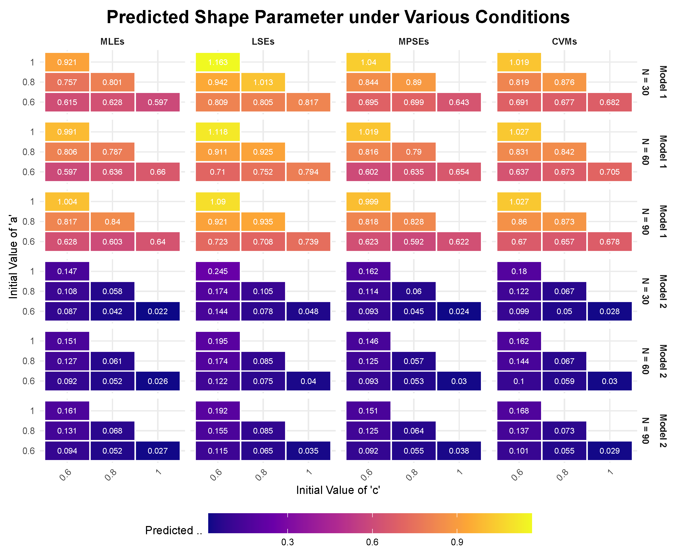
For a normal stress level of S u = 0.05 , we conduct six sets of simulations using different initial values for parameters a and c. From the results presented in Figure 2 (results of Model 1), it is observed that, for the same value of c, the predicted value of η decreases as a decreases. Similarly, for the same value of a, the predicted value of η also decreases with decreasing c.
In Figure 2 (results of Model 2), it is evident that, for the same value of c, the predicted value of η increases with increasing a. In contrast, for the same value of a, the predicted value of η decreases with increasing c due to S u < 1 . Comparing the results from the two models, it is clear that Model 2 provides more stable results and reflects the variations in η u with changes in a and c more accurately. From this perspective, we can conclude that Model 2 is a better fit for the Gompertz distribution under accelerated life testing (ALT).
Based on the estimators obtained for N = 90 , we further calculate the reliability at t 0 = 0.1 , 0.25 , 0.5 , 2 , which can be seen in Table 7, and we find that reliability decreases significantly with increasing t 0 . However, under Model 2, reliability exhibits greater stability during longer test durations. This suggests that Model 2 enables more effective reliability analysis over extended time periods. Thus, further reliability analyses based on Model 2 could provide more information over a longer testing period.
To further test the robustness and generalization capability of our proposed stress-life models, we conducted an additional set of simulations where the lifetime data were generated from the SMPoG distribution. The SMPoG distribution includes an additional shape parameter, α , which allows for more complex hazard rate shapes beyond the standard Gompertz model. This part of the study aims to see how well the simple linear model (Model 1) and the inverse power-law model (Model 2) can approximate the underlying stress-life relationship when the true data generating process is more complex.
We designed three distinct scenarios, each considering three stress levels ( S 1 = 0.5 , S 2 = 0.75 , S 3 = 1 ) with 50 samples allocated to each stress level, to evaluate the models under varying conditions. The performance was assessed based on the mean squared error (MSE) of the parameter estimates, with lower MSEs indicating higher accuracy. The simulation results, presented in Table 8, Table 9, Table 10 deliver a clear and consistent message. Across all three scenarios—spanning moderate complexity, higher baseline complexity, and high stress-acceleration effects—the inverse power-law model (Model 2) consistently and decisively outperformed the simple linear model (Model 1). In every case, the MSEs for the key parameters (a, b, c).
And the derived shape parameters η under the inverse power-law model were significantly lower than those of the linear model. The performance gap was particularly stark in Table 10, where the linear model’s rigid structure failed to capture the strong non-linear stress effect, resulting in extremely high estimation errors. In contrast, the inverse power-law model remained robust and accurate throughout.
This systematic outperformance strongly suggests that the Power Law relationship is a more generalizable and reliable choice for modeling the connection between stress and lifetime parameters. Its inherent flexibility allows it to better approximate complex, real-world failure mechanisms, making it the recommended model for practical applications where the underlying stress-life relationship is unknown.
The effect of sample size on parameter estimation was examined from two perspectives: the shape of the sampling distribution and the normality of model residuals.
  • Impact on Sampling Distribution Skewness:
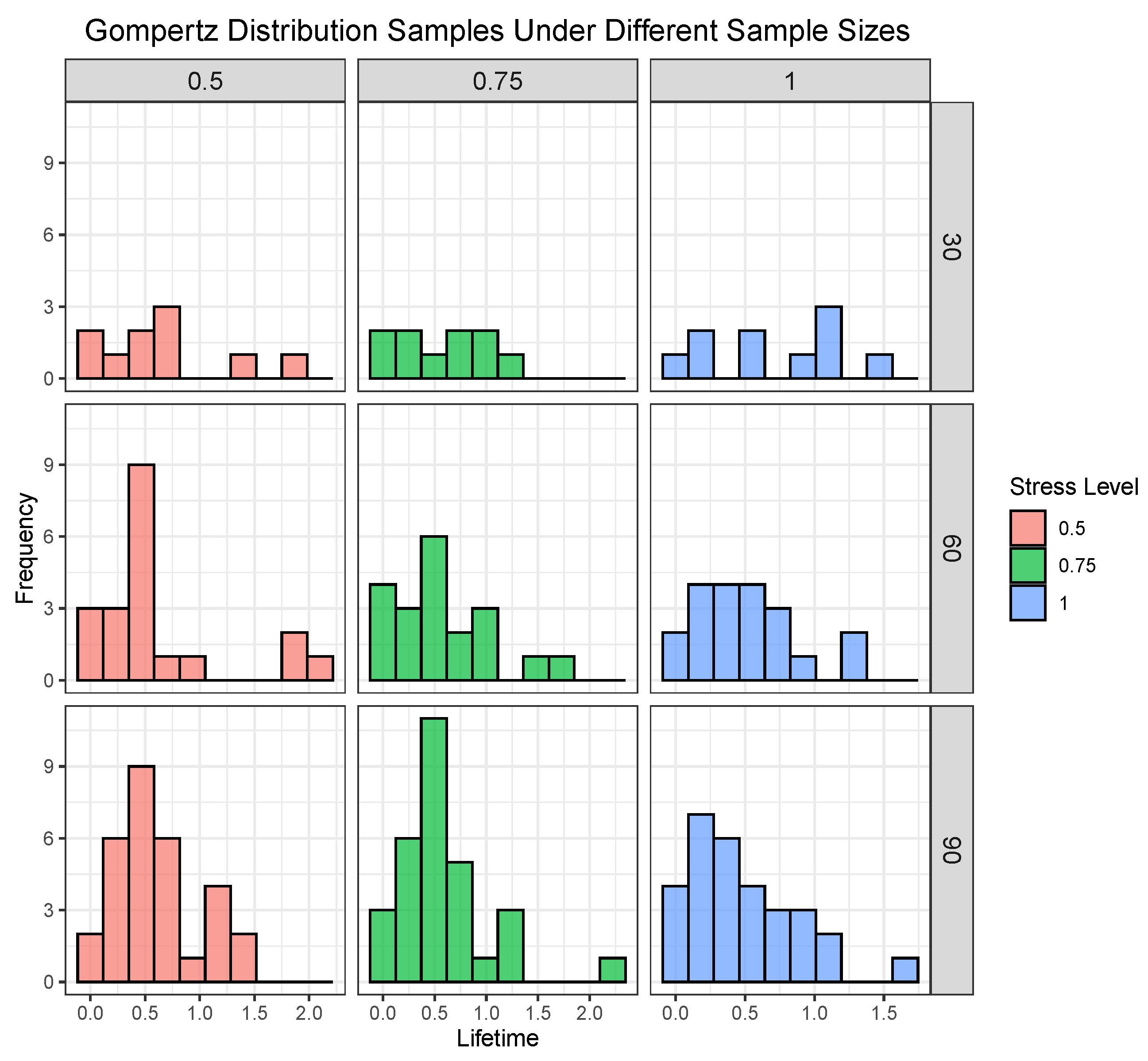
    At low sample sizes ( N = 30 ), the sampling distributions exhibit considerable skewness across multiple stress levels. A notable example is the long tail observed in the S = 0.5 panel, which implies that estimation errors may be partly attributable to the non-symmetric nature of the sampling distribution itself. This issue is substantially alleviated as the sample size grew to 60 and 90, with the distributions becoming increasingly symmetric. Figure 3 and Figure 4 can present these phenomena very clearly. This transition allows for a more direct assessment of the estimator’s capacity, distinct from the artifacts of small-sample distributions.
  • Impact on LSE Residual Normality and Estimator Stability:
    A parallel analysis of the LSE residuals underscore the criticality of sample size. For sparse datasets ( N = 30 and N = 60 ), the residuals are fundamentally non-normal. Formal statistical tests confirmed this observation, yielding values (e.g., for N = 30 , Shapiro–Wilk’s W = 0.004 ) that indicate a complete failure of the normality assumption. This suggests that the estimator is unstable and the residuals are dominated by systematic model misspecification. A watershed moment is observed at N = 90 , where the Shapiro-Wilk statistic jumped to 0.979, signaling that the residual distribution had become highly consistent with normality, which is shown in Figure 5. This convergence highlights that an adequate sample size is a prerequisite for the LSE estimator to achieve stability and robustness.

5. Real Data Analysis

We obtained a real dataset from the Reliasoft website (http://www.reliasoft.com/newsletter/lq2002/qalt.htm, (accessed on 6 January 2025)), which has been previously analyzed in studies conducted by Abdel Ghaly [17] and Mazen Nassar [19]. This dataset records complete failure times, and therefore no censoring is present. We use liquid density as the stress levels (1 g/mL and 1.4 g/mL) and record the failure times (in years) of a pump’s motor. The collected data are presented in Table 11. We analyze the data by calculating the Kolmogorov–Smirnov (K–S) distances and corresponding p-values for each stress level. Table 12 demonstrates the strong overall performance of the model at two stress levels, 1 g/mL and 1.4 g/mL. For 1 g/mL, the K–S distance is 0.3113, accompanied by a p-value of 0.2868, indicating a good fit between the distributions. At 1.4 g/mL, the model shows even greater fitness, with a smaller K–S distance of 0.1928 and a significantly higher p-value of 0.7854, reflecting a closer match. While both stress levels exhibit satisfactory results, 1.4 g/mL exhibits a superior fit. In this study, we only use Model 2 to estimate the parameters.
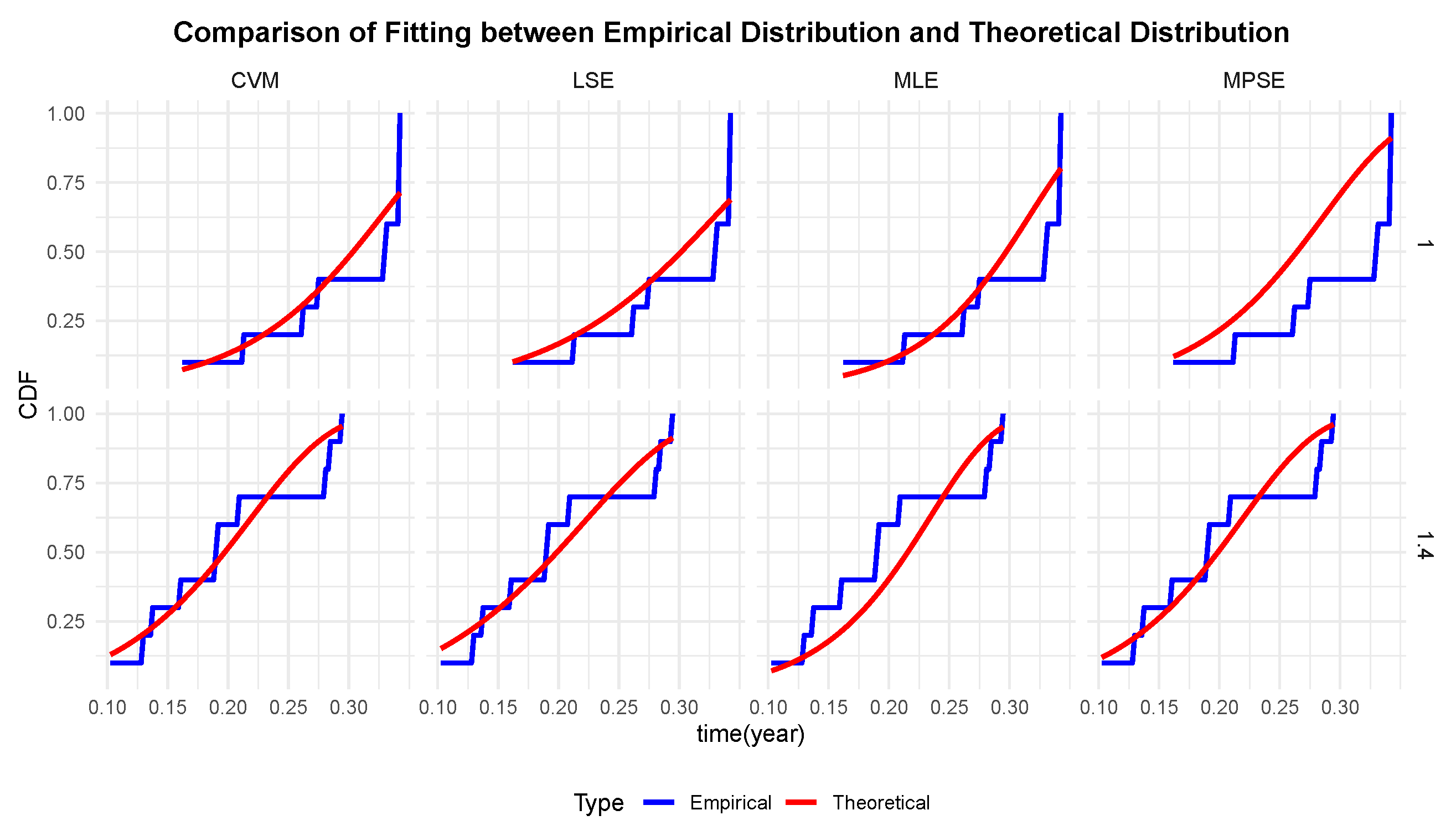
We use the four previously mentioned methods to estimate the parameters a, b, c, η 1 , and η 2 of the Gompertz distribution under Model 2. A summary of these estimation results is provided in Table 13. The comparison between the theoretical cumulative distribution curves and empirical data points under varying stress conditions is visually apparent in Figure 6, which directly demonstrates the fitness of the Gompertz model. To further assess the performance of different estimation methods for Model 2, we conducted AIC (Akaike Information Criterion) [24] comparisons. As shown in Table 14, the MLE method yields the highest Log−Likelihood value (27.44) and the smallest AIC value (−48.89) among the four methods, indicating a relatively better fit in terms of this criterion. Specifically, the AIC values for LSE, MPSE, and CVM are −45.12, −45.78, and −47.25, respectively, which are larger (less negative) than that of MLE. This AIC comparison provides additional evidence for evaluating the suitability of each estimation method when applied to Model 2.
To assess the generalization performance of models and the performance of different parameter estimation methods, we conducted leave- one-out cross-validation and analyzed metrics like MAE, MSE, RMSE, and CV, which can be learned from Table 15. Regarding method performance, MLE excels in accuracy, boasting the lowest MSE (0.00500) and RMSE (0.0707), which means it minimizes both average and extreme prediction errors. MPSE shows the best stability with the smallest CV (0.770), yet it lags in accuracy as indicated by higher MAE, MSE, and RMSE. LSE has a slightly lower MAE (0.0609) than MLE but is less effective in reducing overall error as seen from MSE and RMSE. CVM falls behind MLE in both accuracy and stability. Overall, MLE achieves a favorable balance between accuracy and stability, making it the most suitable method for this context while the model itself proves to have good generalization capability.
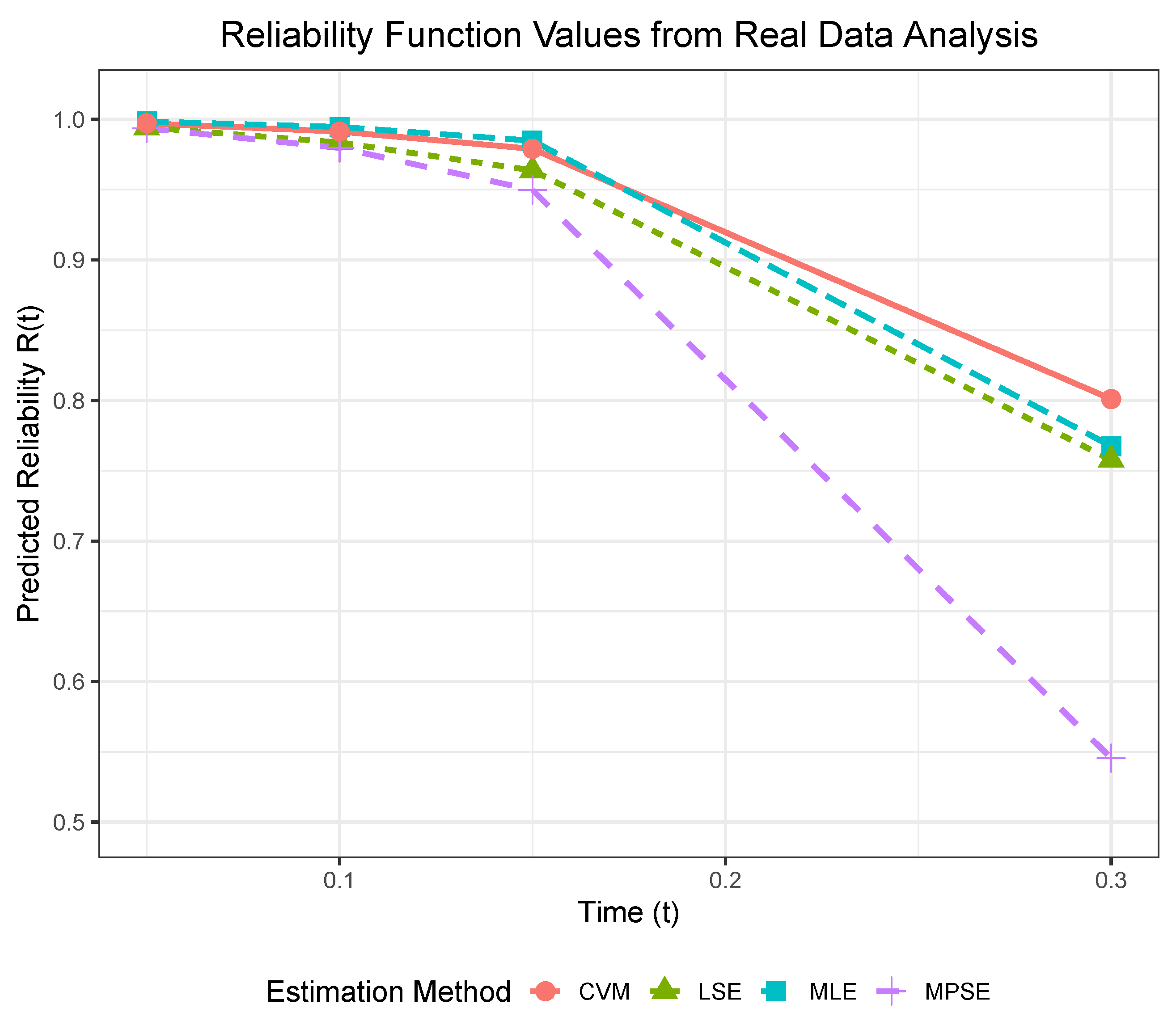
Furthermore, we calculate the K–S distance along with the corresponding p-value of four methods for each dataset unit. We show the results in Table 16. At stress level 1.0, the CVM method performs best, with the lowest K–S distance (0.2871) and the highest p-value (0.3180). The MLE and LSE methods show similar and relatively good performance, with slightly higher K–S distances and lower p-values. The MPSE method performs the worst, having the highest K–S distance (0.4567) and the lowest p-value (0.0200). At stress level 1.4, the LSE method achieves smallest K–S distance (0.1705) and the highest p-value (0.8880). The CVM method ranks second, with a low K–S distance (0.2196) and a high p-value (0.6448). The MLE and MPSE methods show relatively weaker performance. Overall, the CVM method is the best fit at lower stress levels, while the LSE method performs best at higher stress levels. The MPSE method shows poor fitting results under both stress levels. In conclusion, a normal stress level of S u = 0.08 is set to estimate the system parameters under normal conditions. The reliability of the system at t 0 = 0.05 , 0.1 , 0.15 , 0.3 (in years) can be obtained in Table 17, which has been shown in Figure 7 more directly.
6. Conclusions

In this paper, we propose two models to describe the relationship between the shape parameter and stress level in the Gompertz distribution: the simple linear model (Model 1) and the inverse power-law model (Model 2). Additionally, we use four different methods to estimate the parameters of the two models in the Monte Carlo simulations. We obtain the MLEs, LSEs, MPSEs, and CVMs and their mean squared errors for small, medium, and large sample sizes of simulation. Under the same sample size, a novel contribution of this study lies in its systematic comparison of the performance of different parameter estimation methods, as elaborated in Section 4. This focused comparison, using mean squared error (MSE) as a critical metric, reveals nuanced differences in the accuracy and stability of each method, providing valuable insights for method selection in practical applications of Gompertz distribution parameter estimation under constant stress accelerated lifetime tests. After that, we calculate the value of the shape parameter under normal stress conditions and further analyze the reliability at specific time points. However, we observe that Model 2 performs better than Model 1 in Gompertz distribution because the MSEs of the Model 2 are significantly smaller than those of Model 1 under almost all cases, which may reflect simple linear model may perform more unstably. We further analyze the Sine-Modified Power Gompertz (SMPoG) distribution, whose additional shape parameter captures complex hazard behaviors. Model 2 again shows superior fit, justifying its use in real data analysis via the inverse power-law model. So for the real data analysis, we only study the inverse power-law model. Through the results of K–S distance and p-value, we find that the data under 1.4 g/mL perform more suitability. LSE method and CVM methods perform better than the other two methods. Furthermore, Akaike Information Criterion is applied to test the fitness of the model. Leave-one-out cross-validation is employed to further prove the generalizability of this model. Studying the Gompertz acceleration model using censored data would be an interesting direction for further research.

Author Contributions

Conceptualization, S.D. and W.G.; methodology, S.D. and W.G.; software, S.D.; investigation, S.D.; writing—original draft preparation, S.D.; writing—review and editing, W.G.; supervision, W.G. All authors have read and agreed to the published version of the manuscript.

Funding

Wenhao’s work was partially supported by the Science and Technology Research and Development Project of China State Railway Group Company, Ltd. (No. N2023Z020).

Conflicts of Interest

The authors declare no conflicts of interest.

References

  1. Nelson, W. Accelerated Testing: Statistical Model, Test Plan and Data Analysis; Wiley: New York, NY, USA, 2004. [Google Scholar]
  2. Meeker, W.Q.; Escobar, L.A. Statistical Methods for Reliability Data; John Wiley & Sons: New York, NY, USA, 2014. [Google Scholar]
  3. Limon, S.; Yadav, O.P.; Liao, H. A literature review on planning and analysis of accelerated testing for reliability assessment. Qual. Reliab. Eng. Int. 2017, 33, 2361–2383. [Google Scholar] [CrossRef]
  4. Bagdonavicius, V.; Nikulin, M. Accelerated Life Models: Modeling and Statistical Analysis; Chapman and Hall: Boca Raton, FL, USA, 2001. [Google Scholar]
  5. Zhuang, L.; Xu, A.; Wang, B.; Xue, Y.; Zhang, S. Data analysis of progressive-stress accelerated life tests with group effects. Qual. Technol. Quant. Manag. 2023, 20, 763–783. [Google Scholar] [CrossRef]
  6. Hussam, E.; Alharbi, R.; Almetwally, E.M.; Alruwaili, B.; Gemeay, A.M.; Riad, F.H. Single and multiple ramp progressive stress with binomial removal: Practical application for industry. Math. Probl. Eng. 2022, 2022, 9558650. [Google Scholar] [CrossRef]
  7. Ling, M.-H. Optimal constant-stress accelerated life test plans for one-shot devices with components having exponential lifetimes under gamma frailty models. Mathematics 2022, 10, 840. [Google Scholar] [CrossRef]
  8. Nassar, M.; Dey, S. Different estimation methods for exponentiated Rayleigh distribution under constant-stress accelerated life test. Qual. Reliab. Eng. Int. 2018, 34, 1633–1645. [Google Scholar] [CrossRef]
  9. Kumar, D.; Nassar, M.; Dey, S.; Alam, F.M.A. On estimation procedures of constant stress accelerated life test for generalized inverse Lindley distribution. Qual. Reliab. Eng. Int. 2022, 38, 211–228. [Google Scholar] [CrossRef]
  10. Gompertz, B. On the nature of the function expressive of the law of human mortality and on a new mode of determining life contingencies. Philos. Trans. R. Soc. Lond. 1825, 115, 513–585. [Google Scholar]
  11. Winsor, C.P. The Gompertz curve as a growth curve. Proc. Natl. Acad. Sci. USA 1932, 18, 1–8. [Google Scholar] [CrossRef]
  12. Pollard, J.H.; Valkovics, E.J. The Gompertz distribution and its applications. Genus 1992, 48, 15–28. [Google Scholar]
  13. Al-Hussaini, S.F.; Al-Ghamdi, A.N.; El-Morshedy, M.A. The Sine Modified Power-Generated Family of Distributions with Application to Practical Data and Ruin Probability. Symmetry 2023, 15, 2030. [Google Scholar]
  14. Allen, D.M. Mean square error of prediction as a criterion for selecting variables. Technometrics 1971, 13, 469–475. [Google Scholar] [CrossRef]
  15. Jiang, J.; Wang, R. Reliability life prediction of VFD by constant temperature stress accelerated life tests and maximum likelihood estimation. J. Test. Eval. 2009, 37, 316–320. [Google Scholar]
  16. Fan, T.; Yu, C. Statistical inference on constant stress accelerated life tests under generalized gamma lifetime distribution. Qual. Reliab. Eng. Int. 2013, 29, 631–638. [Google Scholar] [CrossRef]
  17. Abdel Ghaly, A.; Aly, H.; Salah, R. Different estimation methods for constant stress accelerated life test under the family of the exponentiated distributions. Qual. Reliab. Eng. Int. 2016, 32, 1095–1108. [Google Scholar] [CrossRef]
  18. Dey, S.; Nassar, M. Generalized inverted exponential distribution under constant stress accelerated life test: Different estimation methods with application. Qual. Reliab. Eng. Int. 2020, 36, 1296–1312. [Google Scholar] [CrossRef]
  19. Dey, S.; Nassar, M. Classical methods of estimation on constant stress accelerated life tests under exponentiated Lindley distribution. J. Appl. Stat. 2020, 47, 975–996. [Google Scholar] [CrossRef]
  20. Harrison, R.L. Introduction to Monte Carlo simulation. AIP Conf. Proc. 2010, 1204, 17. [Google Scholar] [CrossRef]
  21. Dey, S.; Moala, F.; Kumar, D. Statistical properties and different methods of estimation of Gompertz distribution with application. J. Stat. Manag. Syst. 2018, 21, 839–876. [Google Scholar] [CrossRef]
  22. Gill, P.E.; Murray, W. Algorithms for the solution of the nonlinear least-squares problem. SIAM J. Numer. Anal. 1978, 15, 977–992. [Google Scholar] [CrossRef]
  23. Macdonald, P.D.M. Comment on an estimation procedure for mixtures of distributions by Choi and Bulgren. J. R. Stat. Soc. Ser. B 1971, 33, 326–329. [Google Scholar] [CrossRef]
  24. Cavanaugh, J.E.; Neath, A.A. The Akaike information criterion: Background, derivation, properties, application, interpretation, and refinements. Wiley Interdiscip. Rev. Comput. Stat. 2019, 11, e1460. [Google Scholar] [CrossRef]
Figure 1. Density of Gompertz distribution ( η , b).
Applsci 15 09199 g001
Figure 2. The predicted shape parameter under S u = 0.05 and for b = 0.5 .
Applsci 15 09199 g002
Figure 3. Comparison between empirical distribution and theoretical distribution.
Applsci 15 09199 g003
Figure 4. Comparison between empirical distribution and theoretical distribution.
Applsci 15 09199 g004
Figure 5. Residual distribution at N = 90. (Red line: Theoretical quantile reference; Black line: Residual sample quantiles).
Applsci 15 09199 g005
Figure 6. Comparison between empirical distribution and theoretical distribution.
Applsci 15 09199 g006
Figure 7. Reliability function values at different time points.
Applsci 15 09199 g007
Table 1. Parameter estimates of Model 1 for sample size N = 30.
Average Values of Estimates and MSEs (In Parentheses)
Initial ValuesParameterMLEsLSEsMPSEsCVMs
1.0 0.6 0.5a0.887 (1.104)1.129 (1.505)1.034 (1.700)0.985 (1.587)
c0.673 (1.879)0.670 (2.637)0.803 (2.932)0.671 (2.691)
b0.798 (0.257)0.234 (0.111)0.994 (0.358)0.678 (0.463)
η 1 1.224 (0.245)1.464 (0.278)1.401 (0.370)1.320 (0.338)
η 2 1.392 (0.167)1.631 (0.159)1.602 (0.255)1.488 (0.218)
η 3 1.560 (0.325)1.799 (0.370)1.803 (0.507)1.656 (0.435)
0.8 0.6 0.5a0.724 (0.825)0.908 (1.057)0.805 (1.240)0.785 (1.095)
c0.651 (1.515)0.680 (1.971)0.786 (2.301)0.673 (1.972)
b0.744 (0.213)0.252 (0.113)0.913 (0.276)0.661 (0.450)
η 1 1.050 (0.177)1.248 (0.192)1.198 (0.257)1.121 (0.235)
η 2 1.213 (0.137)1.418 (0.129)1.395 (0.197)1.290 (0.175)
η 3 1.375 (0.286)1.588 (0.313)1.591 (0.424)1.458 (0.361)
0.6 0.6 0.5a0.588 (0.564)0.781 (0.775)0.662 (0.868)0.663 (0.801)
c0.549 (0.986)0.552 (1.388)0.657 (1.563)0.553 (1.410)
b0.728 (0.159)0.251 (0.101)0.865 (0.205)0.616 (0.326)
η 1 0.863 (0.133)1.058 (0.151)0.990 (0.193)0.939 (0.176)
η 2 1.000 (0.102)1.196 (0.100)1.155 (0.148)1.077 (0.127)
η 3 1.137 (0.195)1.334 (0.222)1.319 (0.299)1.216 (0.255)
0.6 0.8 0.5a0.591 (0.715)0.766 (0.970)0.655 (1.119)0.638 (0.999)
c0.744 (1.287)0.789 (1.813)0.884 (2.008)0.785 (1.802)
b0.762 (0.204)0.264 (0.111)0.934 (0.278)0.683 (0.475)
η 1 0.963 (0.163)1.160 (0.177)1.097 (0.244)1.030 (0.217)
η 2 1.149 (0.129)1.357 (0.120)1.318 (0.184)1.226 (0.164)
η 3 1.335 (0.255)1.554 (0.289)1.540 (0.374)1.422 (0.336)
0.6 1.0 0.5a0.548 (0.842)0.767 (1.109)0.583 (1.266)0.633 (1.160)
c0.986 (1.473)0.992 (1.974)1.191 (2.267)0.987 (2.005)
b0.772 (0.213)0.228 (0.101)0.958 (0.281)0.658 (0.483)
η 1 1.041 (0.196)1.263 (0.213)1.178 (0.279)1.127 (0.254)
η 2 1.287 (0.150)1.511 (0.135)1.476 (0.210)1.374 (0.177)
η 3 1.534 (0.287)1.759 (0.303)1.774 (0.425)1.620 (0.351)
0.8 0.8 0.5a0.763 (1.023)0.973 (1.324)0.844 (1.550)0.836 (1.347)
c0.766 (1.784)0.802 (2.364)0.924 (2.743)0.799 (2.359)
b0.794 (0.232)0.230 (0.104)0.985 (0.311)0.657 (0.429)
η 1 1.146 (0.219)1.374 (0.239)1.306 (0.320)1.235 (0.278)
η 2 1.338 (0.152)1.574 (0.140)1.537 (0.220)1.435 (0.185)
η 3 1.530 (0.307)1.775 (0.336)1.768 (0.462)1.635 (0.388)
Table 2. Parameter estimates of Model 2 for sample size N = 30.
Average Values of Estimates and MSEs (In Parentheses)
Initial ValuesParameterMLEsLSEsMPSEsCVMs
1.0 0.6 0.5a0.969 (0.143)1.138 (0.159)1.129 (0.219)1.039 (0.185)
c0.629 (0.583)0.513 (0.485)0.648 (0.672)0.585 (0.655)
b0.704 (0.137)0.276 (0.098)0.815 (0.166)0.592 (0.249)
η 1 0.649 (0.093)0.815 (0.106)0.747 (0.134)0.716 (0.116)
η 2 0.795 (0.071)0.964 (0.071)0.916 (0.101)0.859 (0.089)
η 3 0.969 (0.143)1.138 (0.159)1.129 (0.219)1.039 (0.185)
0.8 0.6 0.5a0.785 (0.098)0.944 (0.119)0.921 (0.152)0.855 (0.134)
c0.663 (0.577)0.564 (0.469)0.696 (0.645)0.650 (0.648)
b0.671 (0.085)0.281 (0.083)0.757 (0.110)0.564 (0.185)
η 1 0.507 (0.050)0.649 (0.068)0.582 (0.074)0.562 (0.074)
η 2 0.634 (0.043)0.786 (0.049)0.734 (0.062)0.693 (0.059)
η 3 0.785 (0.098)0.944 (0.119)0.921 (0.152)0.855 (0.134)
0.6 0.6 0.5a0.591 (0.053)0.726 (0.067)0.693 (0.078)0.649 (0.072)
c0.639 (0.574)0.539 (0.497)0.669 (0.658)0.628 (0.692)
b0.630 (0.061)0.286 (0.066)0.699 (0.070)0.530 (0.124)
η 1 0.386 (0.028)0.510 (0.043)0.444 (0.041)0.435 (0.046)
η 2 0.480 (0.024)0.610 (0.031)0.556 (0.033)0.530 (0.034)
η 3 0.591 (0.053)0.726 (0.067)0.693 (0.078)0.649 (0.072)
0.6 0.8 0.5a0.588 (0.051)0.712 (0.064)0.693 (0.078)0.639 (0.070)
c0.883 (0.550)0.737 (0.460)0.913 (0.606)0.851 (0.646)
b0.630 (0.058)0.308 (0.068)0.694 (0.068)0.544 (0.125)
η 1 0.330 (0.024)0.440 (0.034)0.382 (0.035)0.372 (0.037)
η 2 0.449 (0.022)0.569 (0.030)0.523 (0.033)0.493 (0.033)
η 3 0.588 (0.051)0.712 (0.064)0.693 (0.078)0.639 (0.070)
0.6 1.0 0.5a0.600 (0.052)0.714 (0.068)0.708 (0.077)0.644 (0.074)
c1.110 (0.601)0.898 (0.508)1.124 (0.681)1.043 (0.730)
b0.621 (0.052)0.310 (0.066)0.693 (0.066)0.538 (0.117)
η 1 0.291 (0.021)0.397 (0.030)0.344 (0.032)0.331 (0.030)
η 2 0.430 (0.021)0.544 (0.029)0.505 (0.033)0.471 (0.031)
η 3 0.600 (0.052)0.714 (0.068)0.708 (0.077)0.644 (0.074)
0.8 0.8 0.5a0.785 (0.091)0.930 (0.111)0.916 (0.135)0.844 (0.123)
c0.872 (0.572)0.729 (0.509)0.911 (0.669)0.844 (0.724)
b0.659 (0.078)0.302 (0.085)0.753 (0.099)0.579 (0.179)
η 1 0.446 (0.045)0.576 (0.059)0.510 (0.065)0.494 (0.064)
η 2 0.602 (0.040)0.741 (0.048)0.692 (0.057)0.651 (0.056)
η 3 0.785 (0.091)0.930 (0.111)0.916 (0.135)0.844 (0.123)
Table 3. Parameter estimates of Model 1 for sample size N = 60.
Average Values of Estimates and MSEs (In Parentheses)
Initial ValuesParameterMLEsLSEsMPSEsCVMs
1.0 0.6 0.5a0.961 (0.546)1.086 (0.697)0.986 (0.679)0.996 (0.723)
c0.603 (0.903)0.630 (1.196)0.655 (1.131)0.629 (1.201)
b0.655 (0.105)0.329 (0.105)0.815 (0.129)0.583 (0.214)
η 1 1.263 (0.128)1.402 (0.147)1.314 (0.155)1.310 (0.167)
η 2 1.414 (0.088)1.559 (0.096)1.478 (0.105)1.467 (0.114)
η 3 1.564 (0.161)1.717 (0.195)1.642 (0.197)1.625 (0.211)
0.8 0.6 0.5a0.777 (0.377)0.881 (0.502)0.784 (0.478)0.801 (0.513)
c0.580 (0.635)0.609 (0.871)0.641 (0.812)0.608 (0.875)
b0.632 (0.086)0.347 (0.107)0.779 (0.114)0.579 (0.203)
η 1 1.067 (0.088)1.186 (0.108)1.104 (0.108)1.105 (0.120)
η 2 1.212 (0.063)1.338 (0.074)1.264 (0.076)1.257 (0.087)
η 3 1.357 (0.117)1.490 (0.149)1.425 (0.145)1.409 (0.164)
0.6 0.6 0.5a0.567 (0.260)0.679 (0.344)0.568 (0.319)0.606 (0.348)
c0.608 (0.460)0.611 (0.609)0.671 (0.576)0.611 (0.612)
b0.616 (0.069)0.354 (0.090)0.736 (0.082)0.560 (0.150)
η 1 0.872 (0.062)0.985 (0.077)0.904 (0.073)0.912 (0.084)
η 2 1.024 (0.049)1.137 (0.058)1.072 (0.057)1.064 (0.066)
η 3 1.176 (0.094)1.290 (0.115)1.239 (0.114)1.217 (0.125)
0.6 0.8 0.5a0.598 (0.350)0.713 (0.447)0.593 (0.427)0.634 (0.450)
c0.755 (0.609)0.774 (0.786)0.832 (0.759)0.774 (0.791)
b0.633 (0.078)0.338 (0.094)0.768 (0.092)0.558 (0.158)
η 1 0.975 (0.081)1.100 (0.095)1.009 (0.094)1.021 (0.101)
η 2 1.164 (0.061)1.294 (0.067)1.218 (0.070)1.214 (0.075)
η 3 1.353 (0.117)1.487 (0.137)1.426 (0.140)1.408 (0.148)
0.6 1.0 0.5a0.613 (0.424)0.746 (0.552)0.602 (0.528)0.657 (0.562)
c0.945 (0.793)0.950 (1.015)1.044 (0.988)0.955 (1.024)
b0.621 (0.083)0.314 (0.101)0.767 (0.105)0.552 (0.190)
η 1 1.086 (0.089)1.221 (0.109)1.124 (0.108)1.135 (0.121)
η 2 1.322 (0.070)1.459 (0.078)1.385 (0.084)1.373 (0.093)
η 3 1.558 (0.149)1.696 (0.174)1.646 (0.183)1.612 (0.193)
0.8 0.8 0.5a0.745 (0.461)0.883 (0.622)0.743 (0.588)0.800 (0.641)
c0.843 (0.850)0.846 (1.124)0.930 (1.094)0.840 (1.128)
b0.642 (0.101)0.323 (0.100)0.798 (0.127)0.568 (0.210)
η 1 1.166 (0.102)1.306 (0.124)1.208 (0.125)1.220 (0.141)
η 2 1.377 (0.082)1.518 (0.085)1.440 (0.098)1.430 (0.102)
η 3 1.588 (0.168)1.729 (0.187)1.672 (0.208)1.640 (0.204)
Table 4. Parameter estimates of Model 2 for sample size N = 60.
Average Values of Estimates and MSEs (In Parentheses)
Initial ValuesParameterMLEsLSEsMPSEsCVMs
1.0 0.6 0.5a0.976 (0.060)1.085 (0.078)1.034 (0.075)1.026 (0.082)
c0.623 (0.254)0.573 (0.256)0.653 (0.284)0.617 (0.302)
b0.598 (0.047)0.354 (0.074)0.692 (0.053)0.525 (0.102)
η 1 0.642 (0.037)0.738 (0.049)0.665 (0.042)0.680 (0.050)
η 2 0.809 (0.030)0.911 (0.040)0.847 (0.034)0.850 (0.042)
η 3 0.976 (0.060)1.085 (0.078)1.034 (0.075)1.026 (0.082)
0.8 0.6 0.5a0.792 (0.043)0.875 (0.054)0.839 (0.052)0.822 (0.056)
c0.610 (0.266)0.539 (0.274)0.636 (0.301)0.581 (0.321)
b0.579 (0.043)0.373 (0.064)0.659 (0.049)0.526 (0.083)
η 1 0.528 (0.029)0.612 (0.041)0.549 (0.034)0.560 (0.041)
η 2 0.659 (0.023)0.743 (0.031)0.692 (0.027)0.689 (0.032)
η 3 0.792 (0.043)0.875 (0.054)0.839 (0.052)0.822 (0.056)
0.6 0.6 0.5a0.588 (0.027)0.658 (0.034)0.626 (0.033)0.615 (0.034)
c0.620 (0.260)0.562 (0.284)0.638 (0.288)0.605 (0.334)
b0.568 (0.027)0.391 (0.045)0.638 (0.032)0.521 (0.056)
η 1 0.386 (0.014)0.452 (0.021)0.407 (0.017)0.411 (0.020)
η 2 0.486 (0.013)0.554 (0.017)0.515 (0.016)0.511 (0.017)
η 3 0.588 (0.027)0.658 (0.034)0.626 (0.033)0.615 (0.034)
0.6 0.8 0.5a0.588 (0.023)0.655 (0.030)0.631 (0.030)0.613 (0.030)
c0.810 (0.231)0.722 (0.265)0.830 (0.256)0.781 (0.310)
b0.566 (0.025)0.393 (0.044)0.638 (0.031)0.519 (0.053)
η 1 0.340 (0.011)0.405 (0.018)0.361 (0.015)0.365 (0.017)
η 2 0.462 (0.011)0.528 (0.016)0.493 (0.015)0.486 (0.015)
η 3 0.588 (0.023)0.655 (0.030)0.631 (0.030)0.613 (0.030)
0.6 1.0 0.5a0.589 (0.021)0.651 (0.028)0.649 (0.033)0.613 (0.028)
c1.037 (0.229)0.934 (0.242)1.029 (0.254)1.008 (0.285)
b0.558 (0.023)0.395 (0.040)0.655 (0.033)0.512 (0.047)
η 1 0.293 (0.009)0.350 (0.014)0.332 (0.020)0.314 (0.014)
η 2 0.435 (0.010)0.496 (0.015)0.484 (0.022)0.457 (0.014)
η 3 0.589 (0.021)0.651 (0.028)0.649 (0.033)0.613 (0.028)
0.8 0.8 0.5a0.802 (0.042)0.884 (0.054)0.851 (0.051)0.836 (0.056)
c0.862 (0.248)0.780 (0.254)0.902 (0.279)0.842 (0.299)
b0.568 (0.033)0.370 (0.055)0.647 (0.039)0.513 (0.069)
η 1 0.448 (0.019)0.522 (0.027)0.462 (0.022)0.475 (0.026)
η 2 0.621 (0.019)0.700 (0.025)0.650 (0.022)0.650 (0.026)
η 3 0.802 (0.042)0.884 (0.054)0.851 (0.051)0.836 (0.056)
Table 5. Parameter estimates of Model 1 for sample size N = 90.
Average Values of Estimates and MSEs (In Parentheses)
Initial ValuesParameterMLEsLSEsMPSEsCVMs
1.0 0.6 0.5a0.973 (0.356)1.059 (0.471)0.966 (0.415)0.996 (0.478)
c0.610 (0.586)0.627 (0.773)0.653 (0.691)0.627 (0.777)
b0.590 (0.063)0.371 (0.094)0.727 (0.076)0.544 (0.138)
η 1 1.278 (0.084)1.373 (0.107)1.292 (0.096)1.309 (0.114)
η 2 1.430 (0.057)1.530 (0.069)1.455 (0.066)1.466 (0.078)
η 3 1.583 (0.104)1.686 (0.129)1.619 (0.123)1.623 (0.138)
0.8 0.6 0.5a0.787 (0.246)0.891 (0.330)0.786 (0.285)0.830 (0.333)
c0.597 (0.427)0.592 (0.567)0.635 (0.501)0.594 (0.569)
b0.577 (0.053)0.356 (0.083)0.688 (0.062)0.514 (0.116)
η 1 1.086 (0.057)1.187 (0.074)1.103 (0.065)1.128 (0.078)
η 2 1.235 (0.043)1.335 (0.053)1.262 (0.048)1.276 (0.058)
η 3 1.384 (0.082)1.483 (0.102)1.421 (0.094)1.425 (0.108)
0.6 0.6 0.5a0.598 (0.169)0.694 (0.223)0.592 (0.195)0.641 (0.221)
c0.590 (0.282)0.574 (0.367)0.625 (0.328)0.574 (0.369)
b0.558 (0.041)0.368 (0.075)0.659 (0.050)0.509 (0.098)
η 1 0.893 (0.044)0.981 (0.058)0.905 (0.049)0.929 (0.059)
η 2 1.041 (0.034)1.124 (0.044)1.061 (0.038)1.072 (0.046)
η 3 1.189 (0.060)1.267 (0.076)1.218 (0.068)1.216 (0.080)
0.6 0.8 0.5a0.562 (0.217)0.667 (0.301)0.548 (0.248)0.616 (0.308)
c0.826 (0.396)0.817 (0.528)0.877 (0.458)0.811 (0.531)
b0.585 (0.049)0.367 (0.081)0.697 (0.058)0.519 (0.120)
η 1 0.976 (0.048)1.075 (0.067)0.986 (0.054)1.021 (0.073)
η 2 1.182 (0.038)1.279 (0.049)1.206 (0.042)1.224 (0.055)
η 3 1.389 (0.077)1.483 (0.097)1.425 (0.089)1.427 (0.104)
0.6 1.0 0.5a0.590 (0.271)0.689 (0.372)0.569 (0.313)0.628 (0.380)
c0.996 (0.495)0.992 (0.664)1.059 (0.579)0.994 (0.666)
b0.585 (0.053)0.373 (0.088)0.710 (0.063)0.537 (0.125)
η 1 1.088 (0.061)1.186 (0.081)1.099 (0.069)1.125 (0.087)
η 2 1.337 (0.049)1.434 (0.060)1.363 (0.055)1.373 (0.066)
η 3 1.586 (0.098)1.682 (0.122)1.628 (0.114)1.622 (0.128)
0.8 0.8 0.5a0.801 (0.334)0.896 (0.443)0.787 (0.391)0.834 (0.451)
c0.770 (0.563)0.777 (0.762)0.821 (0.668)0.775 (0.766)
b0.590 (0.060)0.370 (0.084)0.723 (0.068)0.540 (0.126)
η 1 1.186 (0.076)1.284 (0.095)1.197 (0.086)1.222 (0.101)
η 2 1.378 (0.053)1.478 (0.063)1.403 (0.059)1.416 (0.070)
η 3 1.571 (0.101)1.672 (0.127)1.608 (0.116)1.609 (0.135)
Table 6. Parameter estimates of Model 2 for sample size N = 90.
Average Values of Estimates and MSEs (In Parentheses)
Initial ValuesParameterMLEsLSEsMPSEsCVMs
1.0 0.6 0.5a0.993 (0.042)1.064 (0.053)1.023 (0.048)1.021 (0.053)
c0.607 (0.140)0.572 (0.154)0.638 (0.157)0.602 (0.173)
b0.551 (0.031)0.392 (0.057)0.634 (0.036)0.512 (0.068)
η 1 0.656 (0.023)0.722 (0.032)0.661 (0.026)0.679 (0.032)
η 2 0.830 (0.021)0.898 (0.029)0.846 (0.024)0.854 (0.029)
η 3 0.993 (0.042)1.064 (0.053)1.023 (0.048)1.021 (0.053)
0.8 0.6 0.5a0.789 (0.028)0.849 (0.037)0.811 (0.032)0.812 (0.038)
c0.599 (0.157)0.567 (0.174)0.625 (0.176)0.595 (0.194)
b0.548 (0.023)0.412 (0.044)0.621 (0.027)0.515 (0.049)
η 1 0.525 (0.016)0.578 (0.023)0.530 (0.018)0.543 (0.023)
η 2 0.660 (0.014)0.716 (0.020)0.673 (0.016)0.679 (0.020)
η 3 0.789 (0.028)0.849 (0.037)0.811 (0.032)0.812 (0.038)
0.6 0.6 0.5a0.590 (0.016)0.633 (0.021)0.611 (0.021)0.603 (0.021)
c0.614 (0.144)0.568 (0.170)0.633 (0.156)0.596 (0.189)
b0.544 (0.018)0.432 (0.036)0.616 (0.023)0.519 (0.039)
η 1 0.388 (0.009)0.432 (0.014)0.398 (0.012)0.404 (0.014)
η 2 0.492 (0.008)0.535 (0.012)0.507 (0.012)0.506 (0.012)
η 3 0.590 (0.016)0.633 (0.021)0.611 (0.021)0.603 (0.021)
0.6 0.8 0.5a0.592 (0.015)0.639 (0.020)0.628 (0.024)0.611 (0.020)
c0.815 (0.167)0.764 (0.193)0.815 (0.176)0.803 (0.215)
b0.541 (0.015)0.425 (0.029)0.622 (0.023)0.508 (0.031)
η 1 0.341 (0.008)0.382 (0.011)0.364 (0.014)0.356 (0.011)
η 2 0.466 (0.007)0.511 (0.010)0.496 (0.015)0.482 (0.010)
η 3 0.592 (0.015)0.639 (0.020)0.628 (0.024)0.611 (0.020)
0.6 1.0 0.5a0.602 (0.016)0.643 (0.022)0.676 (0.036)0.617 (0.022)
c1.034 (0.150)0.969 (0.177)0.964 (0.177)1.018 (0.197)
b0.534 (0.015)0.431 (0.028)0.666 (0.034)0.510 (0.031)
η 1 0.297 (0.006)0.333 (0.008)0.364 (0.027)0.309 (0.008)
η 2 0.445 (0.007)0.484 (0.010)0.518 (0.030)0.458 (0.009)
η 3 0.602 (0.016)0.643 (0.022)0.676 (0.036)0.617 (0.022)
0.8 0.8 0.5a0.793 (0.028)0.848 (0.036)0.818 (0.031)0.813 (0.036)
c0.819 (0.155)0.767 (0.180)0.852 (0.172)0.805 (0.201)
b0.548 (0.022)0.418 (0.041)0.617 (0.026)0.516 (0.046)
η 1 0.454 (0.013)0.505 (0.019)0.458 (0.015)0.472 (0.018)
η 2 0.624 (0.013)0.677 (0.018)0.637 (0.015)0.642 (0.018)
η 3 0.793 (0.028)0.848 (0.036)0.818 (0.031)0.813 (0.036)
Table 7. The predicted reliability function R ^ ( t ) under S = 0.05 and b = 0.5 with N = 90 .
Initial ValuesMethod 1 ResultsMethod 2 Results
actMLEsLSEsMPSEsCVMsMLEsLSEsMPSEsCVMs
1.00.60.10.9020.8950.9020.9000.9840.9810.9850.983
0.250.7630.7520.7610.7590.9580.9510.9600.956
0.50.5580.5490.5480.5540.9110.9000.9150.909
20.0220.0390.0110.0240.5560.5590.5440.557
0.80.60.10.9190.9110.9190.9160.9870.9840.9870.986
0.250.8030.7860.8000.7950.9660.9600.9670.964
0.50.6230.6040.6140.6130.9270.9170.9300.925
20.0460.0680.0300.0500.6210.6170.6100.620
0.60.60.10.9380.9290.9380.9340.9900.9880.9910.990
0.250.8450.8280.8440.8370.9750.9700.9760.973
0.50.6960.6730.6910.6830.9480.9380.9480.944
20.0990.1180.0750.0980.7120.6930.6970.701
0.60.80.10.9400.9300.9410.9350.9950.9930.9940.994
0.250.8500.8310.8510.8390.9860.9830.9850.985
0.50.7040.6780.7020.6870.9710.9640.9690.969
20.1010.1240.0760.1000.8310.8150.8050.826
0.61.00.10.9360.9280.9380.9330.9970.9960.9960.997
0.250.8420.8240.8440.8340.9930.9910.9900.992
0.50.6900.6660.6880.6780.9850.9810.9780.984
20.0880.1110.0640.0880.9070.8940.8540.903
0.80.80.10.9170.9090.9180.9140.9930.9910.9930.993
0.250.7980.7830.7970.7920.9820.9780.9830.981
0.50.6140.5980.6070.6060.9620.9540.9630.959
20.0400.0630.0240.0430.7800.7660.7780.775
Table 8. Scenario 1 simulation results (initial values: alpha = 1.2, a = 0.6, c = 0.8, b = 0.5).
ParameterInitial ValueModel 1Initial ValueModel 2
MLEsLSEsMPSEsCVM MLEsLSEsMPSEsCVMs
alpha1.2001.226 (0.441)1.138 (0.422)1.292 (0.429)1.240 (0.498)1.2001.246 (0.456)1.256 (0.592)1.345 (0.611)1.340 (0.656)
a0.6000.589 (0.948)0.612 (0.222)0.685 (0.208)0.638 (0.255)0.6000.575 (0.069)0.594 (0.094)0.632 (0.096)0.614 (0.099)
c0.8000.720 (1.034)0.658 (0.235)0.749 (0.232)0.697 (0.252)0.8000.837 (0.086)0.791 (0.111)0.763 (0.078)0.807 (0.116)
b0.5000.617 (0.158)0.422 (0.174)0.326 (0.141)0.491 (0.204)0.5000.552 (0.050)0.421 (0.074)0.401 (0.063)0.460 (0.075)
eta11.0000.949 (0.387)0.941 (0.225)1.059 (0.217)0.986 (0.254)0.3450.333 (0.031)0.366 (0.049)0.390 (0.049)0.374 (0.051)
eta21.2001.129 (0.301)1.105 (0.271)1.247 (0.265)1.160 (0.302)0.4770.456 (0.047)0.483 (0.070)0.515 (0.071)0.497 (0.072)
eta31.4001.309 (0.343)1.270 (0.347)1.434 (0.342)1.334 (0.380)0.6000.574 (0.069)0.594 (0.094)0.632 (0.096)0.614 (0.099)
Table 9. Scenario 2 simulation results (initial values: alpha = 1.8, a = 0.8, c = 0.6, b = 0.7).
ParameterInitial ValueModel 1Initial ValueModel 2
MLEsLSEsMPSEsCVMs MLEsLSEsMPSEsCVMs
alpha1.8001.513 (0.669)1.405 (0.809)1.718 (0.620)1.473 (0.796)1.8001.485 (0.684)1.455 (0.791)1.642 (0.680)1.506 (0.777)
a0.8000.630 (0.211)0.649 (0.252)0.807 (0.232)0.649 (0.256)0.8000.644 (0.113)0.646 (0.127)0.740 (0.115)0.648 (0.126)
c0.6000.497 (0.173)0.436 (0.180)0.522 (0.184)0.450 (0.187)0.6000.670 (0.081)0.642 (0.104)0.606 (0.068)0.658 (0.111)
b0.7000.994 (0.294)0.877 (0.302)0.642 (0.204)0.970 (0.374)0.7000.894 (0.134)0.786 (0.130)0.679 (0.097)0.850 (0.155)
eta11.1000.879 (0.227)0.867 (0.284)1.069 (0.224)0.874 (0.284)0.5280.418 (0.059)0.439 (0.070)0.505 (0.064)0.436 (0.070)
eta21.2501.003 (0.267)0.977 (0.334)1.199 (0.254)0.987 (0.332)0.6730.536 (0.085)0.548 (0.097)0.629 (0.088)0.547 (0.097)
eta31.4001.127 (0.329)1.086 (0.407)1.330 (0.307)1.100 (0.404)0.8000.644 (0.113)0.646 (0.127)0.740 (0.115)0.648 (0.126)
Table 10. Scenario 3 simulation results (initial values: alpha = 0.8, a = 1.0, c = 1.2, b = 0.4).
ParameterInitial ValueModel 1Initial ValueModel 2
MLEsLSEsMPSEsCVMs MLEsLSEsMPSEsCVMs
alpha0.8000.877 (0.160)0.742 (0.147)0.720 (0.109)0.836 (0.207)0.8001.012 (0.318)0.901 (0.277)0.917 (0.251)1.012 (0.397)
a1.000-0.935 (0.463)0.931 (0.349)1.021 (0.589)1.0001.144 (0.229)1.062 (0.226)1.076 (0.205)1.152 (0.304)
c1.200-1.034 (0.712)1.007 (0.573)1.131 (0.847)1.2001.182 (0.096)1.146 (0.121)1.106 (0.093)1.163 (0.127)
b0.4000.467 (0.189)0.257 (0.196)0.182 (0.123)0.353 (0.255)0.4000.376 (0.058)0.244 (0.094)0.230 (0.071)0.287 (0.100)
eta11.600-1.452 (0.396)1.434 (0.298)1.587 (0.506)0.4350.524 (0.072)0.501 (0.074)0.518 (0.070)0.541 (0.097)
eta21.900-1.711 (0.496)1.686 (0.380)1.870 (0.623)0.7080.823 (0.135)0.773 (0.134)0.791 (0.125)0.836 (0.180)
eta32.200-1.969 (0.685)1.938 (0.534)2.153 (0.846)1.0001.144 (0.229)1.062 (0.226)1.076 (0.205)1.152 (0.304)
Table 11. Times to breakdown for two stress levels.
Stress Level12345678910
1 g/mL0.1620.2120.2610.2740.3290.3310.3420.3420.3420.342
1.4 g/mL0.1030.1290.1370.1590.1900.1920.2090.2810.2840.294
Table 12. K–S distance and p-value for each stress level.
Stress1 g/mL1.4 g/mL
K–S0.31130.1928
p-value0.28680.7854
Table 13. The estimations under four methods.
ParameterMLELSEMPSECVM
a0.0520.2050.1700.111
c4.5534.0083.1674.862
b18.58812.48815.82614.992
η 1 0.0520.2050.1700.111
η 2 0.2390.7890.4940.569
Table 14. AIC comparisons.
MethodLog-LikelihoodAIC
MLE27.44 −48.89 
LSE25.56−45.12
MPSE25.89−45.78
CVM26.62−47.25
The bold value indicates the best value.
Table 15. Performance metrics of different methods.
MethodMAEMSERMSECV
MLE0.06210.005000.07071.05
LSE0.06090.005130.07161.12
CVM0.06110.005230.07231.15
MPSE0.06390.005360.07320.770
Table 16. K–S distance and p-value for each stress level under different methods.
StressMLELSEMPSECVM
1.00.3133 (0.2271)0.3119 (0.2314)0.4567 (0.0200)0.2871 (0.3180)
1.40.2432 (0.5186)0.1705 (0.8880)0.2275 (0.6021)0.2196 (0.6448)
Table 17. Reliability function values at different time points.
tMLELSEMPSECVM
0.050.99850.99420.99360.9972
0.100.99460.98350.97970.9913
0.150.98480.96370.94970.9790
0.300.76750.75770.54550.8010
η ^ u 0.01870.08370.08380.0374
Disclaimer/Publisher’s Note: The statements, opinions and data contained in all publications are solely those of the individual author(s) and contributor(s) and not of MDPI and/or the editor(s). MDPI and/or the editor(s) disclaim responsibility for any injury to people or property resulting from any ideas, methods, instructions or products referred to in the content.