Depthwise-Separable U-Net for Wearable Sensor-Based Human Activity Recognition

Abstract

In wearable sensor-based human activity recognition (HAR), the traditional sliding window method encounters the challenge of multiclass windows in which multiple actions are combined within a single window. To address this problem, an approach that predicts activities at each point in time within a sequence has been proposed, and U-Net-based models have proven to be effective owing to their excellent space-time feature restoration capabilities. However, these models have limitations in that they are prone to overfitting owing to their large number of parameters and are not suitable for deployment. In this study, a lightweight U-Net was designed by replacing all standard U-Net convolutions with depthwise separable convolutions to implement dense prediction. Compared with existing U-Net-based models, the proposed model reduces the number of parameters by 57–89%. When evaluated on three benchmark datasets (MHEALTH, PAMAP2, and WISDM) using subject-independent splits, the performance of the proposed model was equal to or superior to that of all comparison models. Notably, on the MHEALTH dataset, which was collected in an uncontrolled environment, the proposed model improved accuracy by 7.89%, demonstrating its applicability to real-world wearable HAR systems.

1. Introduction

Recent advancements in wearable sensors and smart devices have led to the emergence of human activity recognition (HAR) as an important research area across diverse disciplines [1,2]. In particular, time-series data collected from various sensors, such as accelerometers and gyroscopes embedded in wearable devices, have been widely used in real-life behavior recognition applications, such as sleep state detection [3], disease management [4], smart homes [5], and digital healthcare [6], owing to the advantages of real-time monitoring, low power, privacy protection, and always-on observation.

In sensor-based HAR systems, data collected from wearable devices are continuously recorded in chronological order. Consequently, it is imperative to preprocess the data, divide them into bins, and extract features from each bin. Early HAR research entailed the manual extraction of features from sensor data, followed by their recognition through the implementation of various machine-learning-based classification techniques. In the early 2000s, numerous studies employed feature-extraction-based techniques, including k-nearest neighbors (KNN), decision trees, support vector machine (SVM), and naive Bayes [7].

However, feature-based machine-learning methods have limitations because feature design based on expert domain knowledge is essential for achieving high performance [8]. In particular, the features can easily vary depending on the environment or user, making model development difficult. To address this challenge, deep learning-based methodologies that can automatically discern intricate features have garnered interest [9]. Deep learning models have the advantage of reducing the burden of handcrafted feature extraction while maximizing the expressiveness of the input data. Among these, convolutional neural networks (CNNs) are widely used as models for effectively recognizing simple daily activities and complex sequential actions because of their ability to recognize local patterns.

These HAR models employ a window-labeling approach that partitions sensor time-series data into fixed-length windows and assigns a single label to each window. The labeling strategies employed in this context can be categorized into two distinct approaches: the selection of the poorest class within a given window or the selection of the class at the most recent time point. This results in a multiclass window challenge, wherein samples from disparate activities are amalgamated within a single window and trained with erroneous labels. This is a primary source of suboptimal prediction accuracy, particularly for brief-duration activities, transitions between activities, and infrequent behaviors. A common approach for addressing this multiclass window challenge is to partition time-series data into brief windows. However, the utilization of brief window lengths is suboptimal because of their propensity to prolong data processing and model training times.

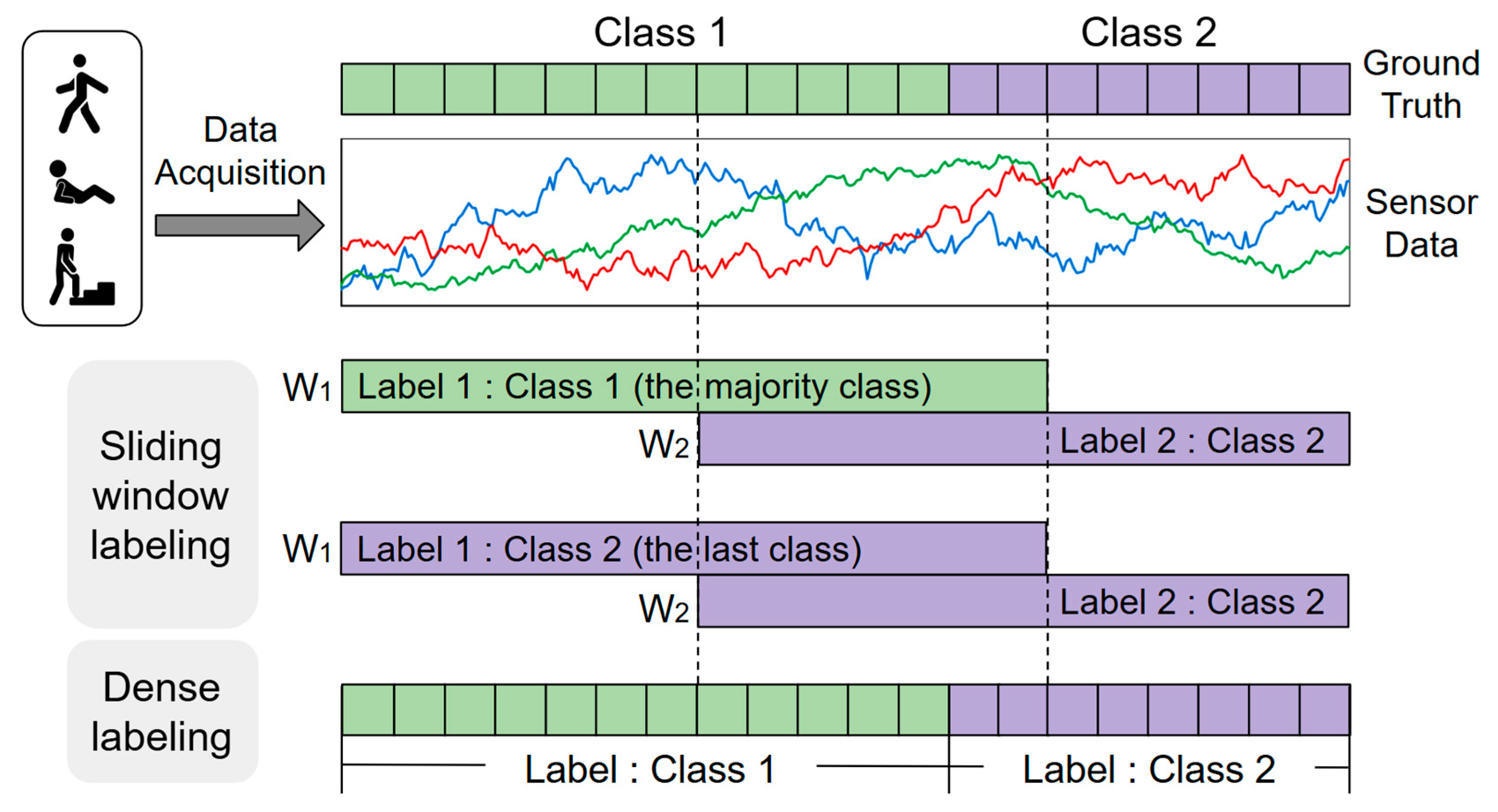
To solve the multiclass window problem, a dense labeling method was introduced to label and predict activities in time steps [10]. Figure 1 is a modified version of the figure from the original study [11] that visually compares the two labeling approaches. The ground truth at the top of Figure 1 shows the true label distribution, which consists of Classes 1 and 2. In sliding window labeling, the entire window is given a single class, despite the fact that there is a mixture of classes within windows W₁ and W₂. Conversely, dense labeling assigns a separate class to each point in time, preserving boundary information and allowing the model to achieve more precise point-by-point recognition.

Dense labeling models based on fully convolutional networks (FCNs) [10] have been proposed to address this challenge. The FCN effectively solves the multiclass window problem by taking the entire time series as the input and predicting the label at each time point (i.e., timestamp). However, owing to their single convolutional structure and relatively shallow network depth, FCNs have a limited ability to effectively capture high-dimensional time series patterns or fine transitions between activities.

Therefore, the encoder–decoder-based U-Net structure for image segmentation was applied to wearable sensor-based HAR. UNet has a structure that compensates for the information lost during downsampling through skip connections and restores the output with the same resolution as the input. This structure can accurately restore information from sensor data at each point in time, which is effective in improving the prediction performance of activity transitions or short activities. Applying U-Net to sensor-based HAR was shown to enable precise point-in-time activity prediction for time-series sensor data [11]. Subsequent approaches, including conditional-UNet [12] and Seq2Dense UNet [13], demonstrated that the U-Net-based encoder–decoder structure is suitable for HAR applications, particularly for recognizing short activities or transitions between different behaviors.

However, existing U-Net-based models contain a large number of parameters, which increases the risk of overfitting in small-scale sensor-data environments and may reduce their applicability in resource-constrained environments. Recent studies have reported that replacing standard convolutions with depthwise separable convolutions can lead to a notable reduction in model parameters while preserving or enhancing action recognition accuracy. This approach addresses the deployment limitations of the existing large CNN models [14,15].

In practical terms, models with fewer parameters and lower computational complexity are more suitable for deployment on resource-constrained platforms such as mobile and edge devices. Lightweight models facilitate real-time execution, improve power efficiency, and allow for scalable deployment in environments with limited memory and compute resources. Consequently, reducing the model size and complexity not only lowers the risk of overfitting in small-scale data environments, but also enhances applicability in real-world scenarios requiring efficient on-device inference and large-scale concurrent service.

Therefore, this study aims to address the key question of whether a depthwise separable convolution-based UNet can maintain frame-level prediction performance while significantly reducing the number of parameters and computational complexity compared to conventional UNet-based models. The contributions of this study are as follows:

-

In this study, we replace all standard convolutions with depthwise separable convolutions in the standard U-Net architecture. This modification reduced the number of trainable parameters by more than 57% compared to the standard U-Net, while maintaining equivalent or superior recognition performance. Notably, the proposed model consistently achieved the lowest number of floating-point operations (FLOPs) among all compared methods, demonstrating that our approach effectively minimizes computational complexity. This lightweight design enables easier deployment on resource-constrained devices such as mobile and edge platforms, facilitates real-time execution, and supports scalable applications in practical contexts with limited resources. In addition, through an ablation study on the performance across network depths, we designed a lightweight U-Net architecture that was optimized for the HAR task.

-

Most existing studies have evaluated models using a subject-dependent segmentation method, in which the same subjects were included in both model training and testing. Conversely, we constructed subject-independent data to strictly evaluate the recognition performance of unseen users in real-world application environments.

-

The proposed model was evaluated using the MHEALTH, PAMAP2, and WISDM benchmark datasets. The evaluation demonstrated the advantages of a lightweight design without performance degradation in key evaluation metrics, such as accuracy, macro-averaged F1-score, and weighted average F1-score, compared with the existing UNet model, while effectively reducing the number of parameters. Specifically, we observed a considerable enhancement in the performance metrics related to MHEALTH data collected in an out-of-lab environment, achieving an accuracy of 0.9259, a macro-averaged F1-score of 0.922, and a weighted average F1-score of 0.923, all of which were higher than those of the comparison models.

The remainder of this paper is organized as follows: Section 2 introduces related studies on sensor-based activity recognition. Section 3 describes the workflow of the experiments and structure of the proposed model, followed by the dataset and the detailed experimental setup. Section 4 presents the experimental results. An ablation study on the proposed model structure is presented in this section. Section 5 provides a discussion, and Section 6 concludes the paper.

2. Related Work

2.1. Sensor-Based HAR Using Sliding Window Labeling

Window-based segmentation is a simple and computationally efficient approach for processing time-series data and has been combined with various traditional machine learning algorithms. Lin et al. [15] utilized the built-in inertial measurement unit (IMU) sensor of a smartphone to monitor the physical state of a user and applied various machine learning algorithms, such as KNN, SVM, naive Bayes, and decision tree, to the extracted statistical and frequency-based features to perform activity recognition with high accuracy.

Since then, deep learning models such as CNN and long short-term memory (LSTM) have emerged, and deep learning-based approaches capable of extracting complex and sophisticated features and learning time-series information have become increasingly popular in the field of sensor-based HAR. Zeng et al. [16] proposed a CNN-based method to effectively extract local features from sensor time-series data, which showed better recognition performance than traditional manual feature extraction methods. Ordonez [17] proposed a DeepConvLSTM structure that combined CNN and LSTM to achieve better human behavior recognition performance than existing single-structure models by utilizing the advantages of both CNN and LSTM to extract local features from sensor time series and learn temporal dependencies, respectively.

With the advancement of deep learning technology, several types of hybrid models have been proposed, such as mixing network structures and introducing attention mechanisms. Ronald [18] proposed iSPLInception, which combines different kernel sizes and inception–ResNet structures to improve the similarity between activities and boundary ambiguity problems in time-series data. Zhang et al. [14] proposed a multi-attribute fusion model that integrates multiscale CNNs and gated recurrent units (GRUs) with kernels of varying sizes and introduced depthwise separable convolution to reduce the weight of the model, achieving higher recognition accuracy and fewer parameters compared with traditional deep learning-based HAR models. Tan [19] proposed a CNN with a multihead attention mechanism (CNN-MHA) model that incorporated multihead attention to solve the long-term dependence problem and achieved an F1-score of 95.7% and a short inference time (0.304 s) on the PAMAP2 dataset. Wei et al. [20] proposed a time convolution network recognition model with attention mechanisms (TCN-attention-HAR) that combines a multiscale TCN and attention mechanisms to overcome the limitations of temporal feature extraction and the challenge of gradient loss with network deepening. Lin et al. [15] proposed a lightweight HAR model, LIMUNet, with depthwise separable convolution and a dual attention mechanism, which achieved 2.9% higher accuracy, 88.3% fewer parameters, and 58.4% less computation than existing lightweight models on the PAMAP2 dataset, and LIMUNet-Tiny demonstrated suitability for edge devices such as smartwatches through further lightweighting. More recently, Mamba-based research has continued, such as the HARMamba model [21], which combines channel-independent patch partitioning with a bidirectional state-space model to improve efficiency and long-term dependence.

These studies adopted a sliding window approach to segment time-series data and assign a single label to each window. Although this is structurally simple, as illustrated in Figure 1, it can lead to mislabeling when multiple activities are included within a single window, resulting in poor classification accuracy. To overcome this limitation, dense labeling approaches that label and predict each time point have recently gained traction.

2.2. Deep Learning Models for Dense Prediction

Because of the multiclass window challenge of traditional sliding window methods, dense labeling approaches that predict activity labels directly at each time point in a time series have been actively studied in recent years. This approach has attracted attention as an alternative to traditional window labeling because it can recognize short activities, activity transitions, and complex behavioral patterns in detail.

Dense labeling was first introduced in the field of sensor-based HAR by Yao et al. [10]. They proposed an FCN-based model that effectively solves the multiclass window problem by taking the entire time series as input and predicting individual labels at each time point. Building on these early works, Zhang et al. [11] were the first to apply U-Net to sensor-based HAR and implemented a model that considers time-series data as single-pixel, multichannel images and makes dense predictions of labels at each time point. They verified the effectiveness of the structure through various hyperparameter settings and experiments and demonstrated excellent performance on several datasets, such as WISDM, UCI HAPT, Opportunity Gesture, and Sanitation. In particular, the U-Net structure has the advantage of restoring information lost during downsampling through skip connections and integrating features at various levels to accurately predict short activity or transition periods and has been used in dense labeling studies since then.

Zhang et al. [12] pointed out the limitations of existing models in reflecting the conditional dependencies between body movements (e.g., head movements during walking), which they defined as the coherent human activity recognition (Co-HAR) problem. By integrating a condition-aware module into the UNet-based model, they modeled the joint probability of multiple activities at each time point to alleviate the problem of interference between multiple activities and improve the precision of dense labeling. In terms of model efficiency, Wen et al. [22] proposed a model that utilizes a modified U-Net++ structure for one-dimensional sensor data to predict time-specific activity classes. They improved the classification accuracy with nested skip connections and deep supervision and achieved 98.2% accuracy on the WISDM dataset while reducing the number of parameters to 0.18 M through pruning. Gaguel et al. [23] pointed out the limitations of window-based classification in that it does not fully reflect contextual information, and dense labeling misses long-term context; they proposed the PrecTime architecture, which combines a sliding window-based CNN-LSTM structure with a CNN-based prediction refinement module and a dual-loss learning strategy. It realizes precise, dense predictions while utilizing window-wise stable context detection and sequence-level context capture.

To address the over-segmentation error, where the same activity is incorrectly split into multiple segments in the transition region, and the boundary prediction instability, Xia et al. [24] proposed a boundary consistency-aware multitask learning framework that learns sample-level activity and boundary predictions concurrently. Meena et al. [13] proposed Seq2Dense U-Net, which combines the advantages of U-Net and a dense layer, and designed a structure that can effectively process time-series data while preserving spatial information, achieving 95.4% and 94.74% accuracies on UCI HAR and HAPT, respectively.

Recently, hybrid models that integrate a self-attention-based transformer encoder with BiLSTM have been attracting attention for their ability to simultaneously enhance time-series contextual information and the precision of each time point prediction [25]. For instance, OnlineTAS [26], which utilizes causal convolution to perform frame-by-frame dense prediction using only past-present inputs for online temporal action segmentation.

3. Materials and Methods

In this section, we describe the complete procedure for the implementation and experimentation of the proposed model. First, we describe the preprocessing process for transforming the raw sensor data into a form suitable for model training and then present the structure and implementation details of the depthwise separable U-Net-based model designed in this study.

3.1. Data Preprocessing

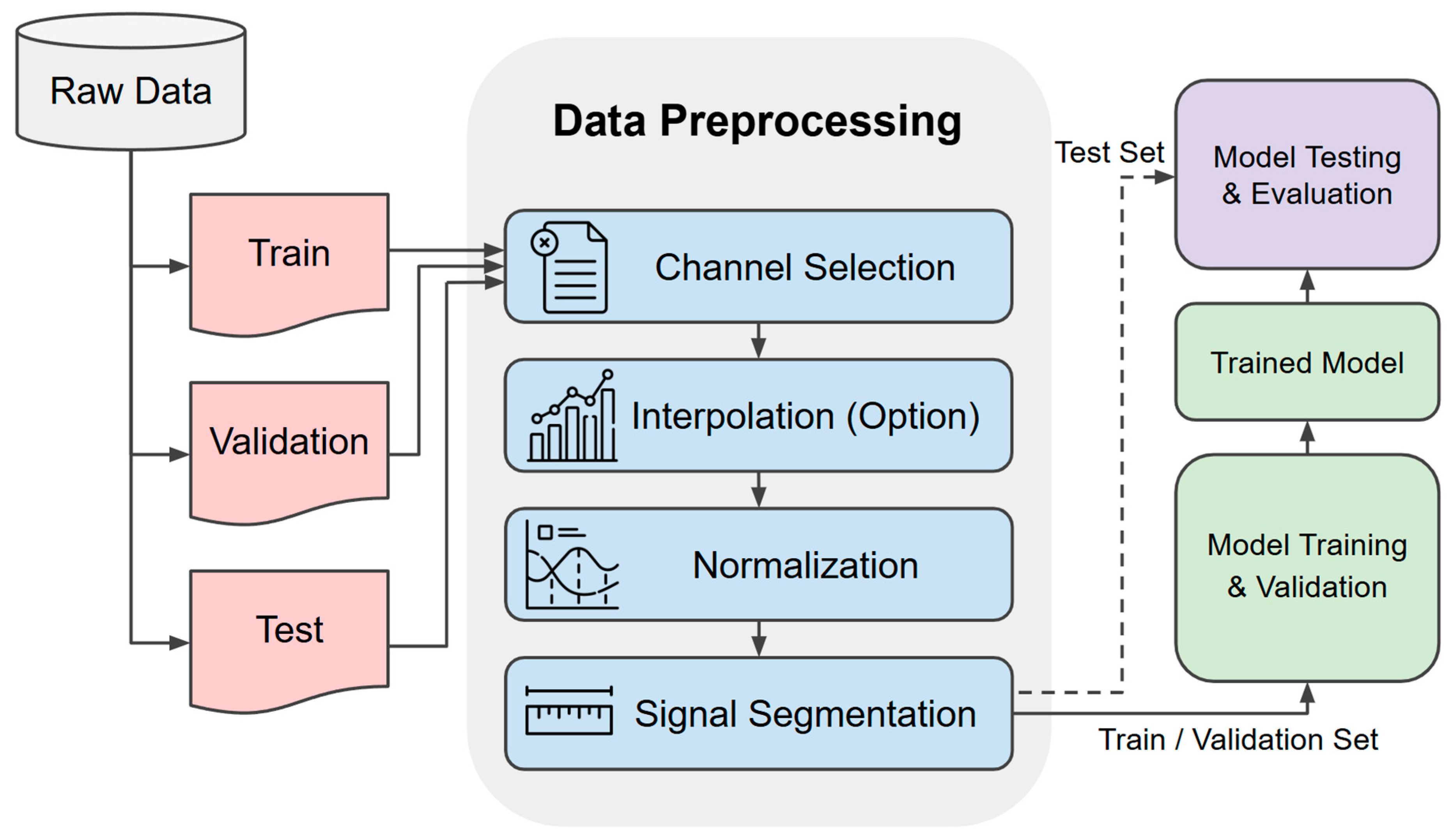
Preprocessing begins with subject-based segmentation followed by channel selection, data normalization, and signal segmentation to construct the model input sequence. The overall data processing flow is illustrated in Figure 2, and each step is described in the following sections.

3.1.1. Subject-Independent Data Split

A common approach for training, validating, and testing deep-learning models is to randomly split the data. However, in HAR, where sensor data are collected for each subject, the activity data of the same subject may be included in both the training and test sets, potentially leading to an overestimation of the model performance [27]. In this study, subject-independent data splitting was adopted to reflect the actual application environment. Data were split based on the subject to ensure that data from the same subject did not overlap between the training and test sets.

3.1.2. Channel Selection and Interpolation

Each dataset had a different number of sensors and channels, and some sensor data were excluded from the experiment because of missing data. In this study, we selected the main sensor channels suitable for the analysis. The selected channels consist of major motion sensors such as accelerometers, gyroscopes, and magnetometers. When necessary, missing data were handled using bilinear interpolation and listwise deletion techniques.

3.1.3. Normalization

Each sensor channel has different physical units and measurement ranges, which, if used without normalization, can cause certain channels to have an undue influence on the model training process. This scale difference affects the loss function calculation and gradient magnitude, thereby reducing the learning stability and convergence speed. To compensate for the distribution differences between the channels and stabilize the model optimization process, $Z$-score normalization was applied. For the input $X$, the mean $\mu$ and standard deviation $\sigma$ are calculated and normalized as shown in Equation (1).

$$Z={\displaystyle \frac{X-\mu }{\sigma }}$$

(1)

Normalization calculates the $Z$-score based on the training set and is applied to the validation and test sets. Each channel was adjusted to a distribution with a mean of zero and a standard deviation of one.

3.1.4. Signal Segmentation

The normalized data were divided into arbitrary window sizes that considered the activity duration and sensor sampling period. Each window is subjected to a dense labeling method to assign individual labels to each point in the time series. Finally, after the segmentation and dense labeling process, the sequence was transformed into (1 × T × C), where T denotes the sequence length and C represents the number of sensor channels, and used as the input to the model.

3.2. Model Architecture

In this study, we propose a lightweight UNet model for time-series-based HAR inspired by the standard UNet structure [28] and depthwise separable convolution [29,30]. A UNet is a structure that produces an output with the same resolution as its input and can effectively perform point-in-time dense predictions. The proposed model reduces the computational complexity by replacing the standard convolution of a traditional UNet with depthwise separable convolution. In addition, a convolutional layer with a 1 × 5 kernel size is added to effectively extract the features of the input time series.

All convolutional layers were followed by batch normalization, rectified linear unit (ReLU) activation functions, and He normal initialization [31]. The input data are considered as a multichannel time series of the form (1 × T × C), defined by a height of 1. The final output of the model is the class probability distribution (B × T × T_c) at each time point, where Tc denotes the number of classes, while maintaining the same time length. All convolutional operations maintained the time-axis length with the same padding, and downsampling was performed using a 1 × 2 max-pooling operation.

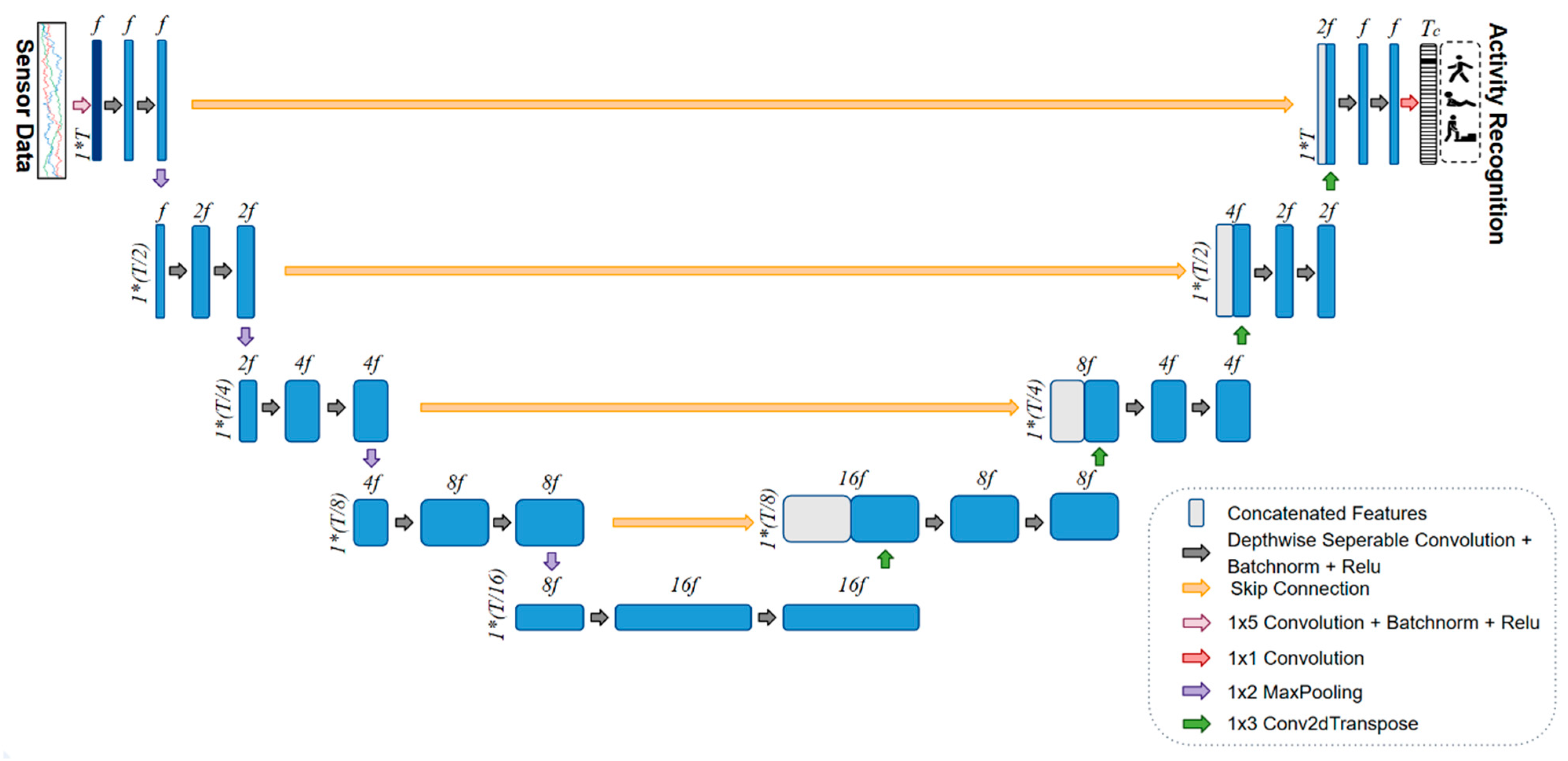
The overall structure of the proposed model is shown in Figure 3. The following subsection describes the depthwise separable convolution applied to reduce the number of parameters in the model, followed by detailed explanations of each network component and the final configuration.

3.2.1. Parameter Reduction Strategy

Depthwise separable convolution is a structure that decomposes standard convolution into two stages to maximize computational efficiency [29]. In the first stage, a depthwise convolution is applied, which separately performs a convolution for each input channel. In the second stage, a pointwise convolution of size 1 × 1 combines the channel information to create new features. Unlike standard convolution, where parameters grow proportionally to the product of filter size, input channels, and output channels, this factorization changes the computation to the sum of the two stages. As a result, this structure can significantly reduce the parameter count and computational cost compared with standard convolution while maintaining a similar level of expressiveness, and has been adopted in a variety of lightweight models.

3.2.2. Initial Convolution Layer

Depthwise separable convolution requires a standard convolution in the preprocessing stage for efficient channel interaction and feature extraction. This design is widely employed in lightweight models, such as MobileNet [29] and Xception [30], and effectively extracts spatial and channel characteristics to ensure computational efficiency and learning stability. The input time series is represented in the form (1 × T × C), with height 1, length T, and the number of sensor channels C. The time series was transformed into a feature map with a base filter size of f by sequentially passing through a 1 × 5 convolution, batch normalization, and ReLU activation in an initial convolutional layer. Every block is then computed based on these channels, and the entire network structure is designed to compress and restore the time-series information based on this feature map.

3.2.3. Encoder–Decoder Network

The proposed model comprises four encoder blocks, four corresponding decoder blocks, and a central bottleneck block. Similarly to UNet, this structure allows the encoder to capture the context of the time series and the decoder to restore the resolution (enabling precise localization). Skip connections pass the details extracted from the encoder to the decoder to supplement the information required for reconstruction.

Each encoder block consists of two depthwise separable convolutions and max pooling, followed by batch normalization and ReLU. The first pointwise convolution doubles the number of channels, and the number of filters doubles with each pass through the encoder block. The length of the time axis is sequentially halved for each pooling operation. The same padding was applied to all convolutions such that the length of the time axis changed only during the pooling or upsampling steps.

In the bottleneck block, depthwise separable convolutions of the same structure are applied twice to produce the most compressed representation. The (1 × T/16 × 16f) feature map passed to the decoder block is subjected to a 1 × 3 transposed convolution to restore the time-axis resolution. Unlike simple interpolation, upsampling via transposed convolution allows for more precise reconstruction using a learnable filter [32]. The combined feature map is then subjected to two depthwise separable convolutions to reduce the number of channels by half. The time length is restored from T/16 to T by passing it through a decoder.

3.2.4. Classification

The final output of the decoder was a feature map (1 × T × f) with restored time-series resolution, which was used to make point-in-time activity predictions. First, a 1 × 1 convolution is applied to convert the number of channels to the number of activity classes T_c. This operation maps the feature vector at each time point to a class-logit vector of the same size. The softmax function was then applied to output a point-in-time class probability distribution of the form (1 × T × T_c), and a dense prediction was made to assign an activity label to every point in the input time series. By extracting features while preserving the resolution of the input time series and making separate predictions at each time point, the proposed model can achieve precise segmentation and activity detection even in sequences where multiple classes coexist.

3.2.5. Network Configuration Strategy

As the model depth increases, more complex patterns can be learned; however, this results in increased computational cost and parameter count. In particular, the UNet structure doubles the number of filters in each block, leading to a significant increase in the total number of parameters. This structural characteristic increases the network’s memory requirements and computation time while also increasing the likelihood of overfitting. Therefore, the model depth should be carefully chosen to balance computational efficiency and performance. In this study, we compared the performance differences across network depths for each dataset and determined that a depth of four provided the optimal structure with the most stable performance. The experimental evidence supporting this finding is described in detail in the ablation study.

3.3. Experimental Design

In this section, the experimental setup used to evaluate the performance of the proposed model is described. We introduce the benchmark datasets and explain the subject-independent data splits and window segmentation for each dataset. The implementation details are described, comparison model configurations are defined, and performance evaluation metrics are specified.

3.3.1. Datasets

Three public datasets—MHEALTH [33], PAMAP2 [34], and WISDM [35]—were employed in this study. These datasets contain labeled information for all sampling points. A brief description of the three datasets is presented in

Table 1. Brief description of datasets.

Dataset	Sampling Frequency	Sensors	Environment	Activity
MHEALTH	50 Hz	3-axis accelerometer (±6 g, ±16 g), gyroscope, magnetometer, 2-lead ECG (chest)	Out-of-lab	Standing still, sitting and relaxing, lying down, walking, climbing stairs, waist bends forward, frontal elevation of arms, knees bending, cycling, jogging, running, and jumping forward and backward *.
PAMAP2	100 Hz (** ~9 Hz)	3-axis accelerometer, gyroscope, magnetometer, heart rate monitor	In-lab	Lying, sitting, standing, walking, running, cycling, Nordic walking, ascending stairs, descending stairs, vacuum cleaning, ironing, and rope jumping.
WISDM	20 Hz	3-axis accelerometer on smartphone	In-lab	Jogging, walking, ascending stairs, descending stairs, sitting, and standing.

* Abbreviated as “Jump front and back” in figures. ** Sampling frequency of the heart rate monitor.

, and each dataset is described in detail below.

1.

MHEALTH

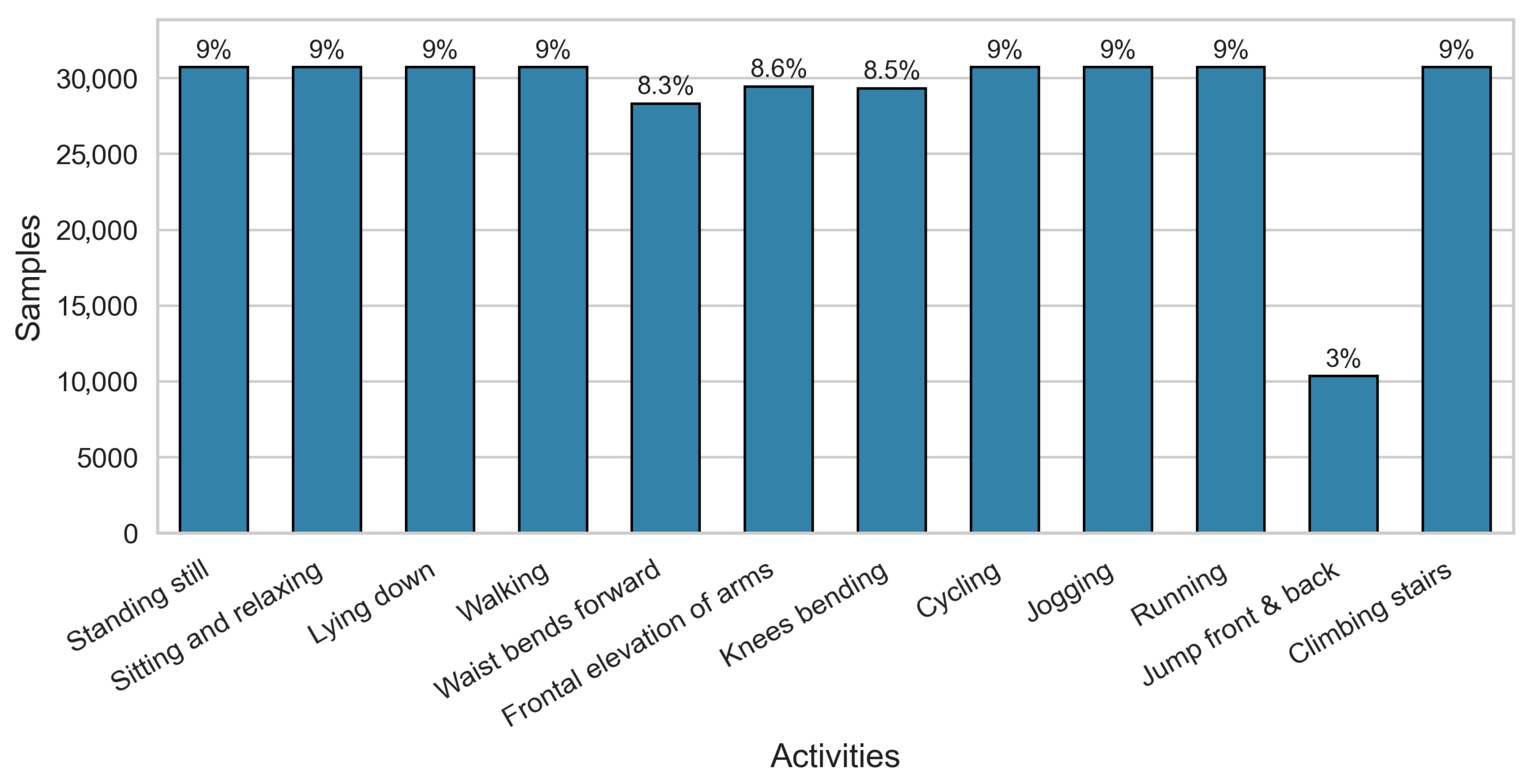
MHEALTH [33] is an HAR benchmark dataset collected by measuring body movements and vital signs of ten subjects. The subjects performed 12 physical activities, and sensors were attached using elastic bands to the chest, right wrist, and left ankle. Each sensor measured tri-axial acceleration, gyroscope, and magnetometer data, whereas the chest sensor recorded a two-channel electrocardiogram (ECG) signal at 50 Hz. The ECG signals were excluded from the analysis because of their limited relevance to activity recognition. The experiment utilized 21 sensor features. All activities were performed in an unconstrained out-of-lab environment. For activity labeling, video recording was performed concurrently, without restrictions on the recording procedure. The distribution of each activity is shown in Figure 4, with the jumping forward and backward activity being disproportionately represented, accounting for only 3% of the total sample.

2.

PAMAP2

The PAMAP2 [34] is a public benchmark dataset comprising nine participants (one female and eight males). The subjects ranged in age from 23 to 31 years old and performed 18 activities according to a protocol while wearing three IMUs and a heart rate monitor attached to the wrist, chest, and ankle. Each IMU contains two 3-axis accelerometers (±6 g, ±16 g), a gyroscope, and a magnetometer collecting data at 100 Hz. In this study, 36 channels extracted from the IMUs were used.

The activities consisted of 12 basic activities (e.g., walking, running, cycling, and ascending and descending stairs) and six optional activities (e.g., driving, working on a computer, and watching TV). We restricted our analysis to the basic activities. The distribution by activity is shown in Figure 5. 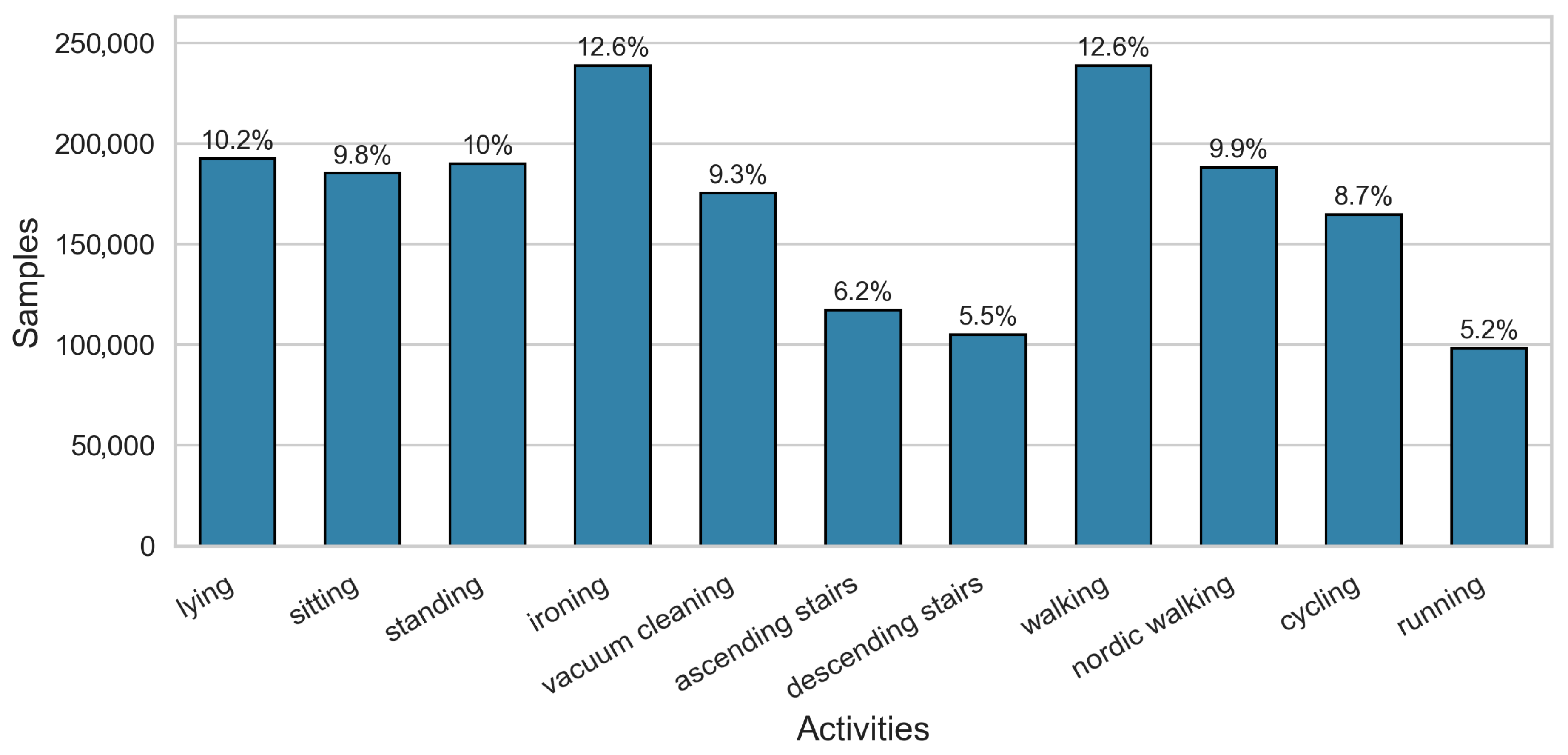Rope jumping was only performed in six out of nine subjects and was excluded from the analysis because of its low sample proportion of 2.5% [36]. The remaining 11 activities exhibited a class imbalance, with ironing, walking, ascending stairs, descending stairs, and running accounting for 12.6%, 12.6%, 6.2%, 5.5%, and 5.2% of the data, respectively. Missing values that occurred during the wireless transmission were replaced by bidirectional linear interpolation to maintain time-series continuity. Finally, the IMU time-series data, after missing-value interpolation and activity filtering, were used for model training.

3.

WISDM

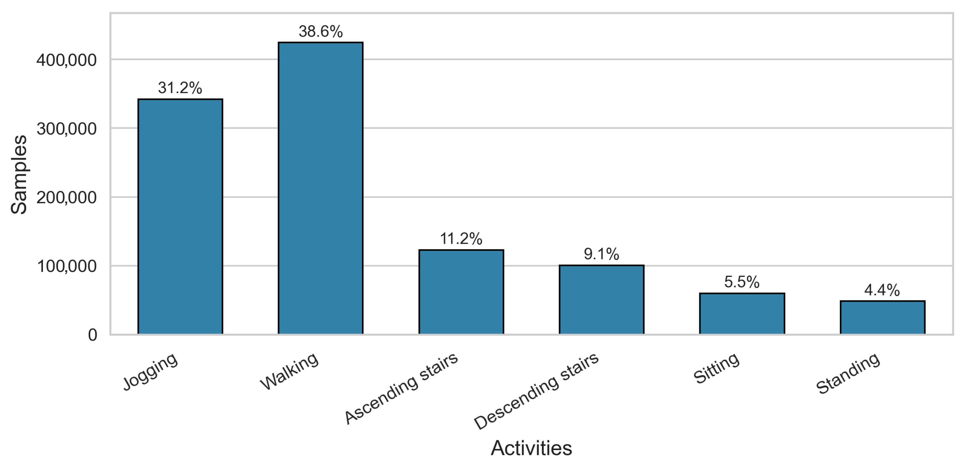
WISDM [35] is an HAR benchmark dataset collected by the Wireless Sensor Data Mining research team. The data was collected from 36 subjects using Android smartphones in their front pockets. Each participant performed six activities (sitting, standing, walking, ascending and descending stairs, and jogging) in a controlled environment. Data were collected at 20 Hz using the smartphone’s built-in 3-axis accelerometer. Each sample contained the user ID, activity label, timestamp, and x/y/z-axis acceleration information. The activity distribution is shown in Figure 6, which shows that jogging and walking accounted for approximately 69.8% of the total samples, indicating a high imbalance across activities.

3.3.2. Data Split and Segmentation

In this section, we describe the data splitting criteria and sliding window-based preprocessing applied to each dataset. As described in Section 3, we used a subject-independent data split to ensure independence between the training, testing, and validation data. We designated MHEALTH Subjects 6 and 10 as the test set, Subjects 2 and 9 as the validation set, and the remaining subjects (1, 3, 4, 5, 7, and 8) as the training set [37]. For the PAMAP2 dataset, we designated Subject 6 as the test set, Subject 5 as the validation set, and the remaining subjects as the training set. For the WISDM dataset, we split Subjects 1–30 into the training set and Subjects 31–36 into the test set [27]. However, because there were no criteria for splitting the validation set, we randomly extracted 10% from the training set.

The window size was set to 128, and the overlap was set to 50% [20]. The window size for MHEALTH and PAMAP2 was set to 128, and that for WISDM was set to 224 for comparison with a previous study [11]. No overlap was applied to the test sets to avoid the problem of duplicate class predictions for the same time step, and the number of subsequences generated after subject-independent split and window segmentation for each dataset is summarized in

Table 2. Data split and segmentation configuration.

Dataset	Window Size	Subjects		Subsequences
MHEALTH	128	Train	1, 3, 4, 5, 7, 8	3239
		Test	6, 10	514
		Validation	2, 9	1090
PAMAP2	128	Train	S01, S02, S03, S04, S07, S08, S09	21,545
		Test	S06	1951
		Validation	S05	4135
WISDM	244	Train	1–30	7218
		Test	31–36	1783
		Validation	10% of train subsequences *	802

* Randomly sampled after window segmentation.

.

3.4. Implementation Details

3.4.1. Equipment and Software

The experiments were conducted on a workstation with an AMD Ryzen 9 3900XT 12-core CPU running at 3.79 GHz, 128 GB of RAM, and an NVIDIA GeForce RTX 2080 Ti GPU with 11 GB of RAM. The workstation ran Windows 10. All implementations were developed in Python 3.8 and used TensorFlow 2.5, CUDA 11.2, and cuDNN 8.1.0 for GPU acceleration.

3.4.2. Learning Parameters

The learning rate for all models was set to 0.001 with a plateau scheduler, and the batch size was 32 [11]. The Adam optimizer was used for the categorical cross-entropy loss. The optimal weights were determined at the epoch with the lowest validation loss. In addition, we set the training epoch to 100 but terminated the training early if the validation loss did not improve for 20 epochs.

3.4.3. Comparison Models

To verify the performance of the proposed model, FCN Yao, UNet, and UNet Zhang were selected as comparison models. Initially, the concept of dense labeling was introduced to the HAR field by Yao [10], who applied semantic segmentation to time-series data. The proposed model utilizes UNet [28] as the fundamental framework. UNet has been extensively employed as a fundamental structural element in sensor-based behavior recognition prediction models. Among these, UNet Zhang [11] is a representative UNet-based dense labeling model that has been extensively cited in the field of sensor-based HAR. This model has demonstrated efficacy on various benchmark datasets and has been employed as a standard for comparison in subsequent studies [38].

The aforementioned learning parameters were applied to all comparison models, and the structural parameters of the other models were reimplemented as outlined in the original paper. In instances where a public code was available, it was utilized without modification. The structural features of each model are as follows.

1.

FCN Yao

The FCN model proposed by Yao et al. [10] utilizes a fully convolutional structure to solve the label ambiguity problem based on a sliding window and performs dense labeling of sequences in an end-to-end manner. It consists of six convolutional layers and a max-pooling layer, including a dropout layer with a dropout rate of 0.1.

2.

UNet

UNet [28] is a proposed model for medical image segmentation that was implemented in this study to perform a dense prediction of time-series data as the basic structure of the proposed model. The model has a symmetric encoder–decoder structure, where each encoder block contains a convolution layer of size 1 × 3, batch normalization, and ReLU activation. Time-axis downsampling was performed with a max pooling of size 1 × 2. The decoder block restores the original temporal resolution with a transposed convolution, and the final output layer applies sigmoid activation to a 1 × 1 convolution to output class probabilities at each time point. Dropouts were not included in the experiment.

3.

UNet Zhang

The UNet proposed by Zhang et al. [11] is a representative UNet-based dense-labeling model in the HAR field. It has a symmetric structure consisting of five blocks for the encoder and decoder, respectively, and the output for prediction at each time point is obtained by a 1 × 1 convolution and sigmoid activation. In this study, a publicly available implementation code was used [39].

3.5. Performance Evaluation

Because all models predicted labels at each point in the input sequence, the performance of these models was evaluated by comparing the predicted and actual values at each sample point. The performance of the model was evaluated based on three key metrics: accuracy, macro-average F1-score, and weighted average F1-score. The macro F1-score is defined as the simple average of the F1-scores of each class, with equal weights assigned to all classes. The weighted F1-score is a metric that calculates an F1-score, which reflects the overall data distribution by weighting the proportion of samples in each class. The definitions of each metric are as follows:

$$\mathrm{A}\mathrm{c}\mathrm{c}\mathrm{u}\mathrm{r}\mathrm{a}\mathrm{c}\mathrm{y}={\displaystyle \frac{\mathrm{T}\mathrm{P}+\mathrm{T}\mathrm{N}}{\mathrm{T}\mathrm{P}+\mathrm{T}\mathrm{N}+\mathrm{F}\mathrm{P}+\mathrm{F}\mathrm{N}}}$$

(2)

$$\mathrm{P}\mathrm{r}\mathrm{e}\mathrm{c}\mathrm{i}\mathrm{s}\mathrm{i}\mathrm{o}\mathrm{n}={\displaystyle \frac{\mathrm{T}\mathrm{P}}{\mathrm{T}\mathrm{P}+\mathrm{F}\mathrm{P}}}$$

(3)

$$\mathrm{R}\mathrm{e}\mathrm{c}\mathrm{a}\mathrm{l}\mathrm{l}={\displaystyle \frac{\mathrm{T}\mathrm{P}}{\mathrm{T}\mathrm{P}+\mathrm{F}\mathrm{N}}}$$

(4)

$$\mathrm{F}1={\displaystyle \frac{2·\mathrm{P}\mathrm{r}\mathrm{e}\mathrm{c}\mathrm{i}\mathrm{s}\mathrm{i}\mathrm{o}\mathrm{n}·\mathrm{R}\mathrm{e}\mathrm{c}\mathrm{a}\mathrm{l}\mathrm{l}}{\mathrm{P}\mathrm{r}\mathrm{e}\mathrm{c}\mathrm{i}\mathrm{s}\mathrm{i}\mathrm{o}\mathrm{n}+\mathrm{R}\mathrm{e}\mathrm{c}\mathrm{a}\mathrm{l}\mathrm{l}}}$$

(5)

$${\mathrm{F}1}_{macro}={\displaystyle \frac{1}{C}}\sum _{i=1}^C{\mathrm{F}1}_i$$

(6)

$${\mathrm{F}1}_{weighted}=\sum _{i=1}^C{w_i·\mathrm{F}1}_i$$

(7)

TP denotes true positive, TN denotes true negative, FP denotes false positive, and FN denotes false negative. C is the total number of classes, i is the class index, ${\mathrm{F}1}_i$ is the F1-score for Class i, and $w_i$ is the proportion of samples belonging to Class i.

In this study, we present the number of trainable parameters to quantitatively demonstrate the reduction in the number of parameters owing to the implementation of depthwise separable convolution. Furthermore, to comprehensively evaluate model efficiency, we measured the theoretical computational complexity in terms of giga-FLOPs (GFLOPs) and the inference time. GFLOPs were computed for a batch size of 1, and inference times were expressed in seconds.

A confusion matrix was also presented, which was used to visually understand the prediction performance between classes and analyze the misclassification in a particular class. The confusion matrix is a useful tool for comparing performance differences between static activities or similar behaviors and provides an intuitive interpretation of the classification ability for each physical activity.

4. Results

In this section, we present and analyze the experimental results for each dataset using tables and performance metrics. Furthermore, the results of the aforementioned ablation study are reported. The objective of the study was to determine the optimal architecture of the proposed model.

4.1. Results of MHEALTH Dataset

Table 3. Performance of the different models on the MHEALTH dataset.

Model	Accuracy	Macro Averaged F1-Score	Weighted Average F1-Score	Trainable Parameters	GFLOPs	Inference Time
FCN Yao	0.8238	0.8274	0.8229	54,636	0.254	1.669
UNet	0.8513	0.8575	0.8441	2,713,036	0.08	1.6274
UNet Zhang	0.846	0.8512	0.839	10,499,052	0.172	1.7216
Proposed	0.9259	0.922	0.923	1,158,508	0.034	1.6765

presents the performance comparison results of the four models for the MHEALTH dataset. The proposed model performed best in terms of accuracy, macro averaged F1-score, and weighted average F1-score. In particular, the accuracy is 92.59%, which is an improvement of 10.21%, 7.46%, and 7.99% over those of FCN Yao (82.38%), UNet (85.13%), and UNet Zhang (84.6%), respectively.

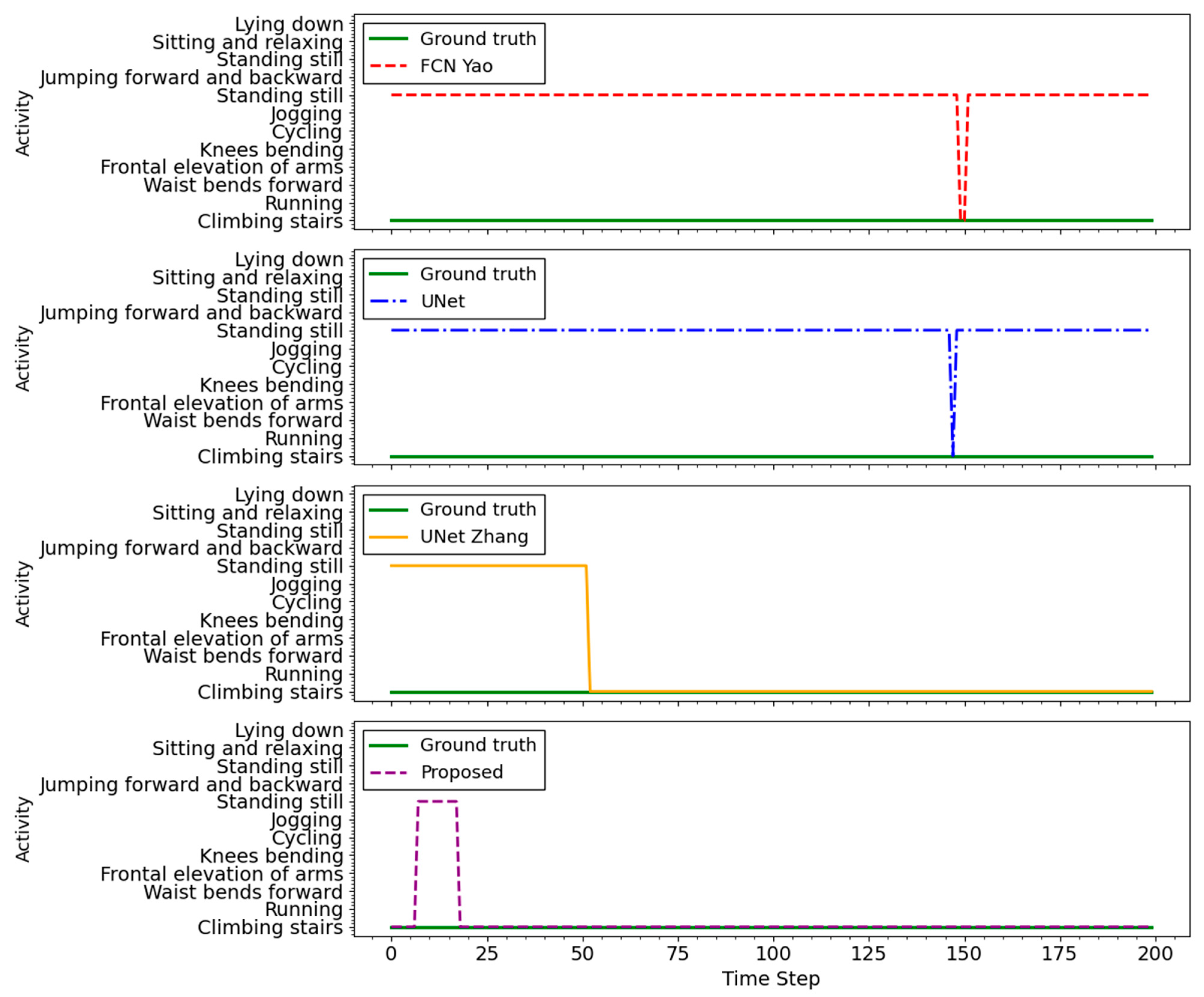
Figure 7 presents a partial example of dense predictions for subject 10 in the test dataset. In this sequence, the ground truth is entirely “Climbing stairs”; nevertheless, the FCN Yao, UNet, and UNet Zhang models consistently misclassify it as “Standing still” in most timesteps, with occasional correct classifications. This confusion is likely due to the static posture phases that occur between steps, the sensor signals of which resemble those of standing. In contrast, the proposed model accurately predicted “Climbing stairs” throughout nearly the entire sequence, demonstrating greater robustness in distinguishing this activity from visually and kinematically similar static activities.

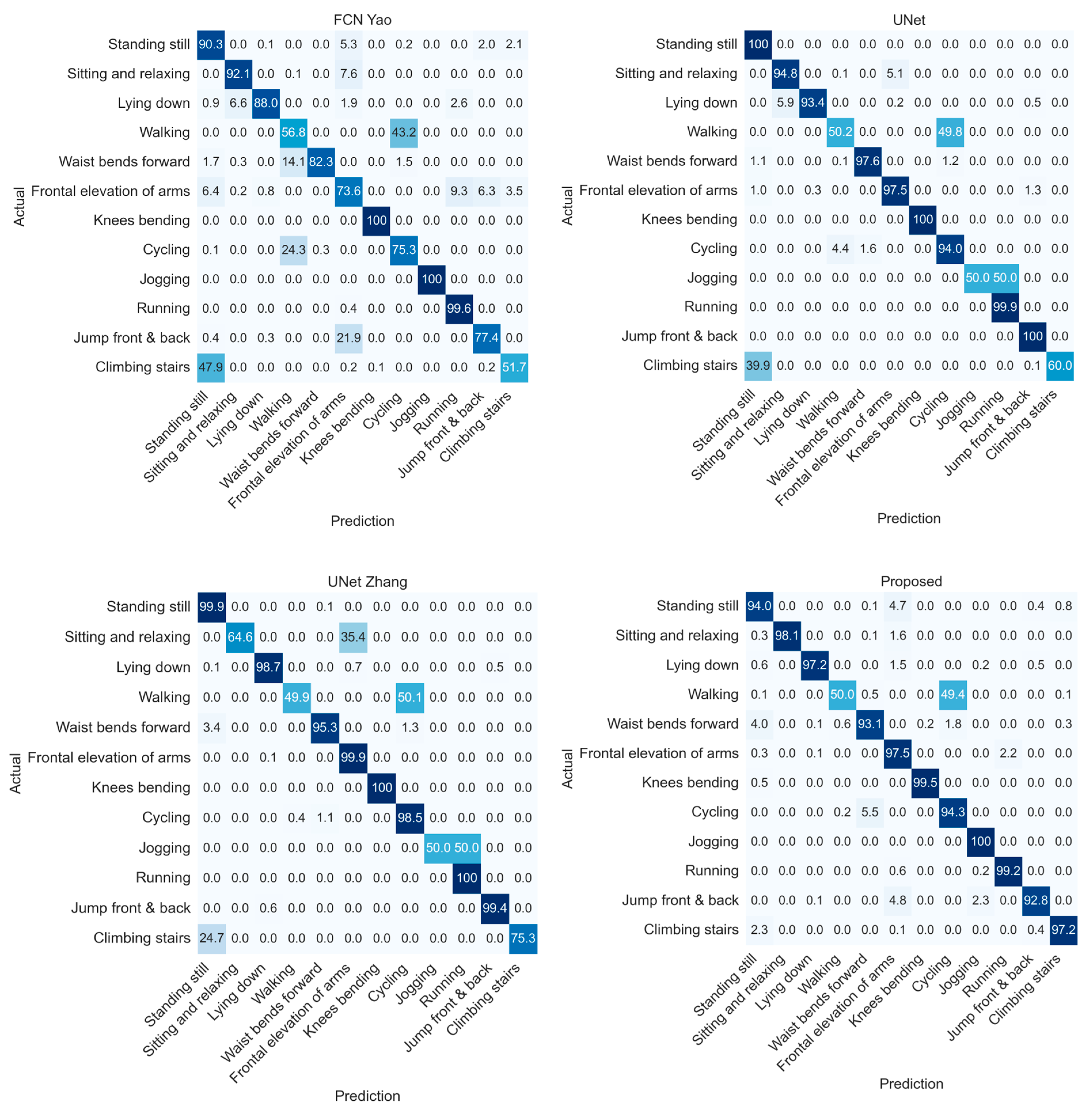
As illustrated in Figure 8, the activity-specific classification performance of each model is presented using a confusion matrix. The performance of all models is poor in terms of accurately identifying “Walking”, with an accuracy of approximately 50%. Additionally, there is a tendency to misclassify “Walking” as “Cycling”. The accuracy of “Climbing stairs” was classified by FCN Yao, UNet, and UNet Zhang with 51.7%, 60%, and 75.3%, respectively, and was confounded with “Standing still”. In contrast, the proposed model achieved an accuracy of 97.2% for classifying “Climbing stairs”.

The UNet Zhang model misclassified “Sitting and relaxing” as “Frontal elevation of arms” at a rate of approximately 35.4%, and both the UNet and UNet Zhang models showed a low accuracy of approximately 50% for the “Jogging” activity. In contrast, the FCN Yao and proposed models classified this activity correctly, achieving a perfect score of 100%. The proposed model has 1,158,508 parameters, which is approximately 88.9% and 57.3% fewer than those of UNet Zhang and UNet, respectively.

Notably, the proposed model also achieved the lowest computational complexity, with a GFLOPs value of only 0.034, compared to 0.254 for FCN Yao, 0.08 for UNet, and 0.172 for UNet Zhang. Despite these reductions, the inference time remained comparable to those of other models, indicating that the substantial decreases in parameter count and computational cost did not negatively impact inference speed.

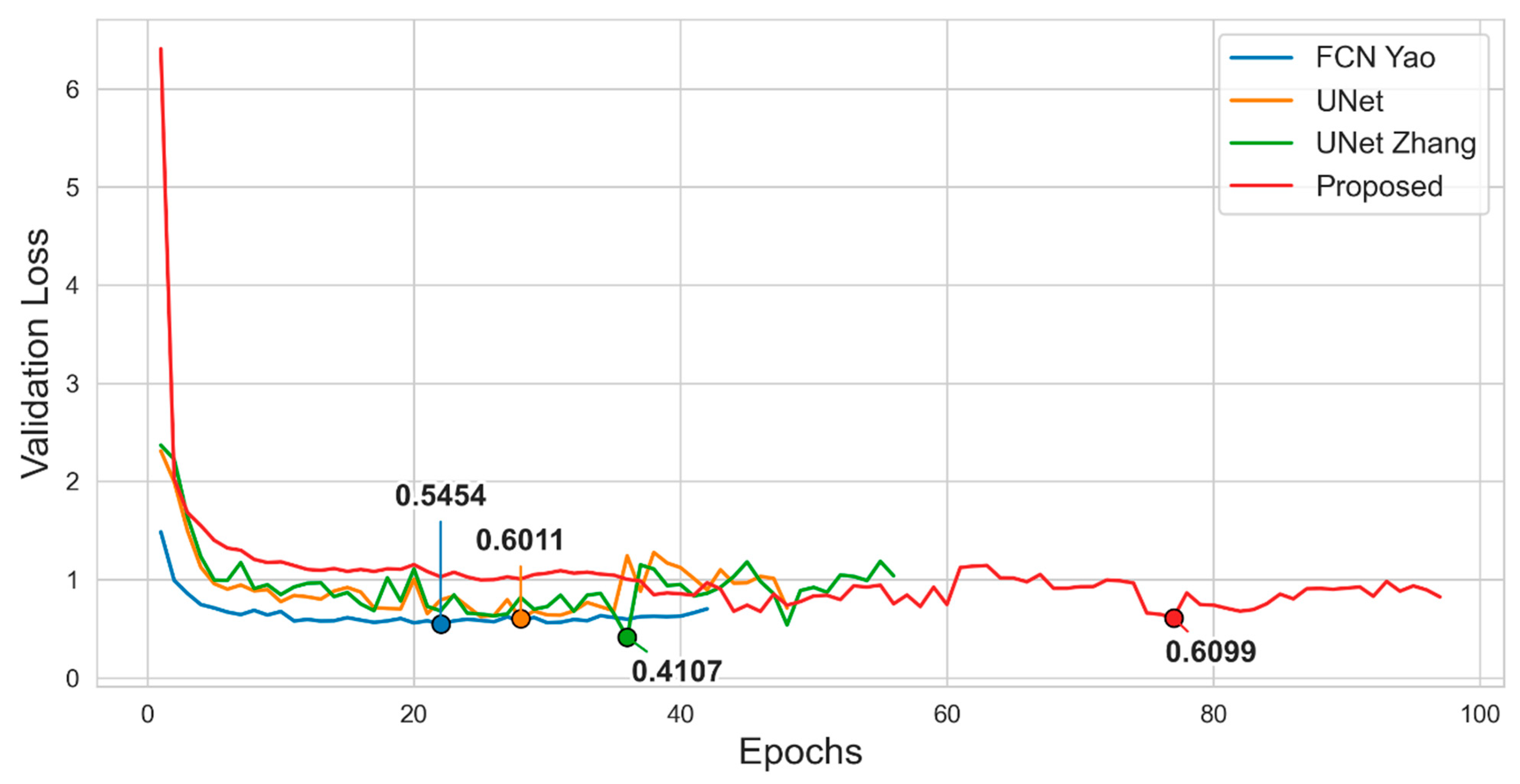
Figure 9 illustrates the change in validation loss for each model on the MHEALTH dataset. The proposed model converged slowly over the entire epoch, reaching the lowest validation loss at the end, whereas the UNet Zhang and FCN Yao models converged more rapidly, with UNet Zhang achieving the lowest validation loss of 0.4107. However, the proposed model performed best across all evaluation metrics. This suggests that the relative magnitude of the validation loss values or speed of convergence may not necessarily correspond to the actual predictive performance of the model. In addition to the well-known fact that determining the optimal weight of a model based solely on the minimum validation loss does not necessarily guarantee optimal performance [40], this discrepancy can be attributed to several factors.

As previously illustrated in Figure 4, the MHEALTH dataset has a fairly even class distribution, but the minority classes “Jumping forward and backward” are underrepresented. Prediction errors in these minority classes are sensitive to validation loss but may have a limited impact on the weighted F1-score or accuracy. In addition, this study applied a subject-independent split, which led to activity-specific distributional differences between the validation and test sets, as shown in Figure 10. However, these factors alone do not fully explain the discrepancy between the validation loss and key performance metrics.

A more fundamental cause is that the pattern of misclassification between similar activities, such as walking, cycling, climbing stairs, and standing still, is different for each model, as indicated in the confusion matrix results. This confusion between similar classes is reflected sensitively in cross-entropy when calculating the validation loss, but its impact on the overall performance can be relatively mitigated in classification-based metrics such as accuracy or F1-score. In conclusion, the proposed model did not exhibit a lower validation loss or faster convergence; however, it outperformed the other models on all metrics.

4.2. Results of PAMAP2 Dataset

Table 4. Performance of the different models on the PAMAP2 dataset.

Model	Accuracy	Macro Averaged F1-Score	Weighted Average F1-Score	Trainable Parameters	GFLOPs	Inference Time
FCN Yao	0.8209	0.7969	0.8103	59,243	0.435	6.7803
UNet	0.8488	0.8303	0.8409	2,714,443	0.081	6.5998
UNet Zhang	0.8488	0.8316	0.8378	10,500,459	0.173	6.6366
Proposed	0.8659	0.8465	0.8545	1,160,875	0.034	6.6467

presents the performance comparison of the four models on the PAMAP2 dataset. The proposed model achieved the highest performance across all key metrics. Specifically, the accuracy is 86.59%, which is a 1.8% improvement over UNet (84.79%) and UNet Zhang (84.79%).

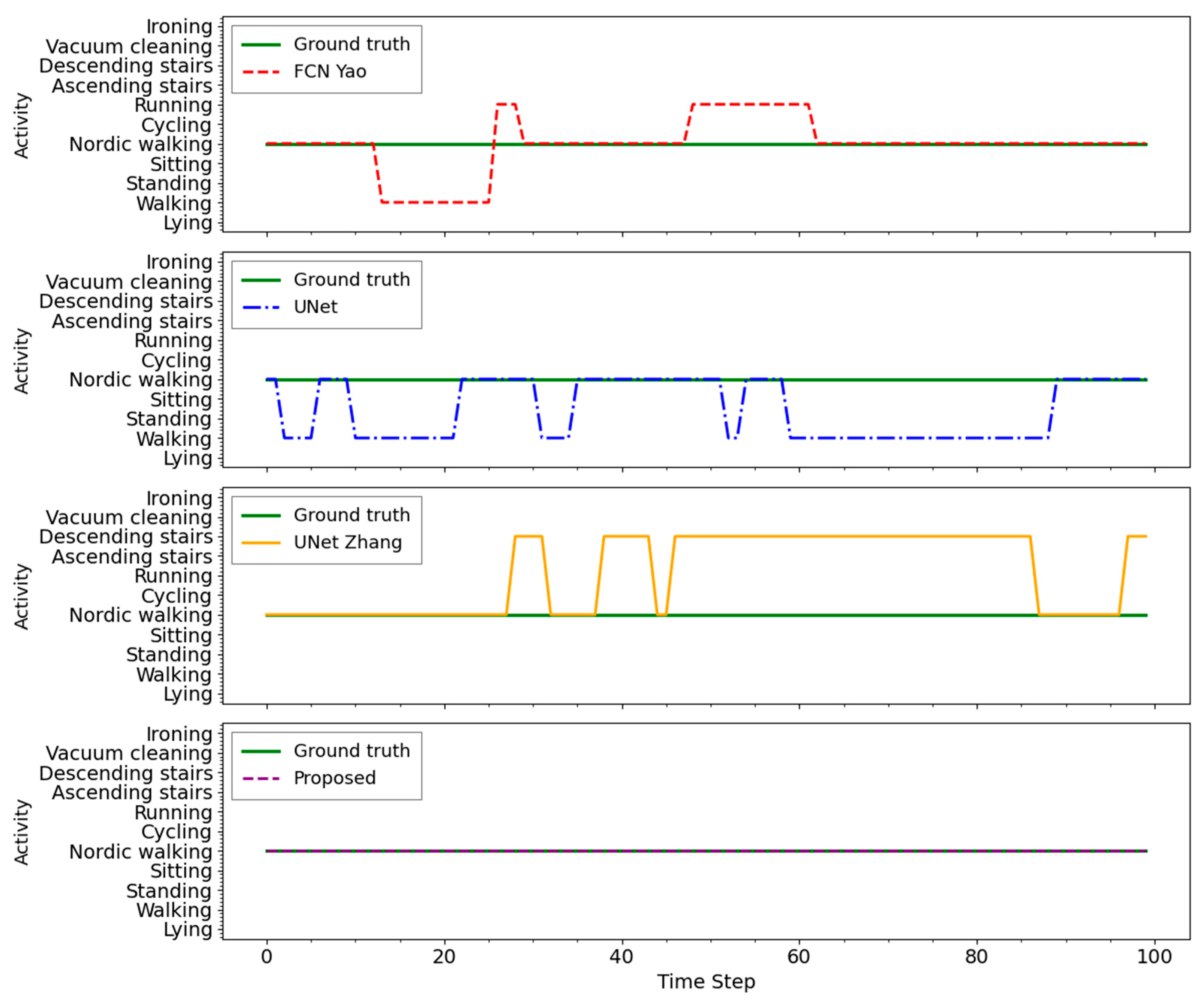
Figure 11 shows an example of dense prediction taken from subject S06 in the test dataset. The ground truth sequence consists entirely of Nordic walking; however, other models frequently predicted it as walking or, in the case of UNet, descending stairs in certain segments. These misclassifications are plausible, given the similarity in motion patterns between Nordic walking and these activities, particularly in lower-body movements. However, the proposed model consistently predicted Nordic walking throughout the sequence, demonstrating greater stability when handling activities with overlapping motion characteristics.

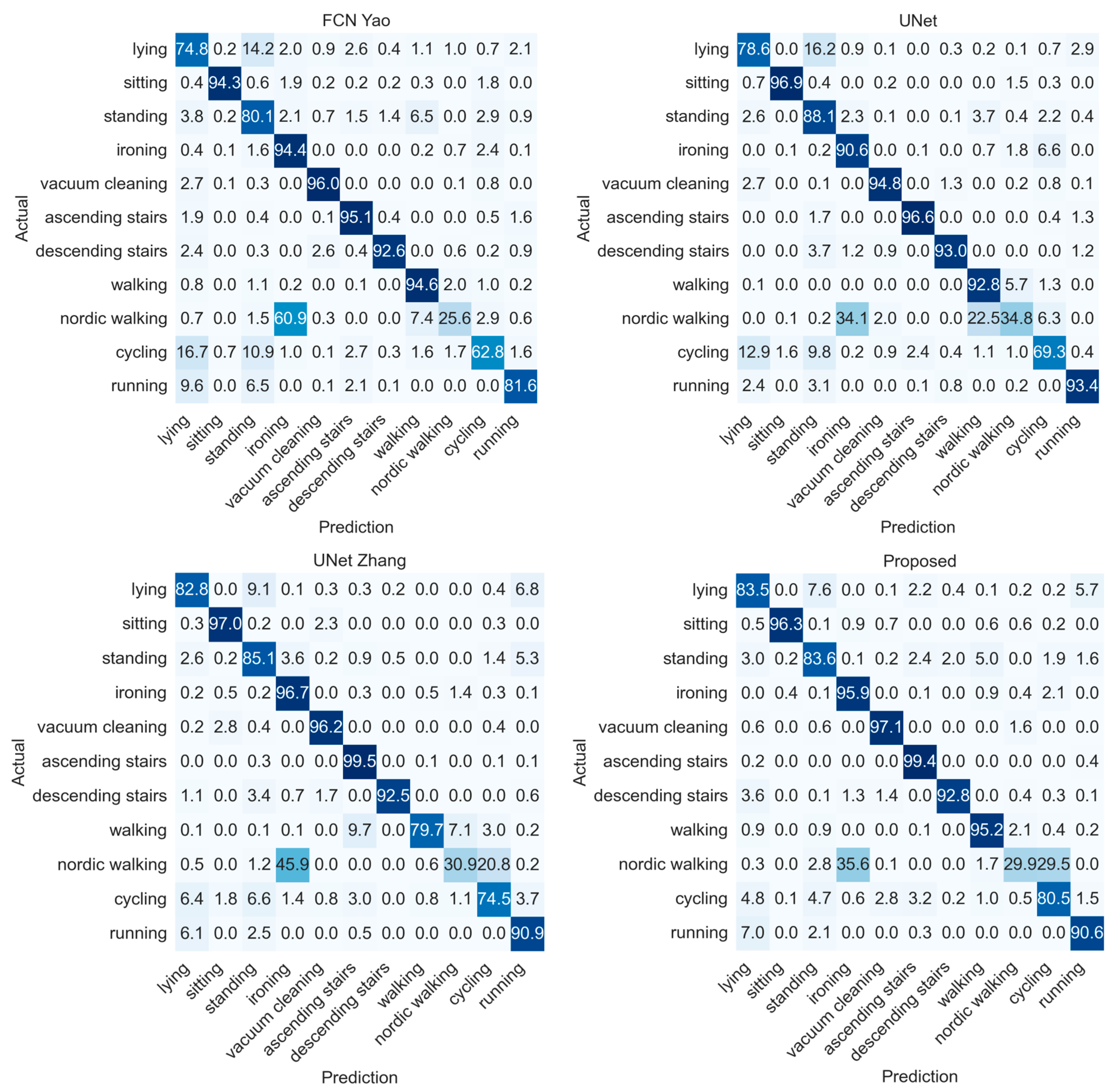
According to the confusion matrix in Figure 12, Nordic walking was the most challenging activity to classify across all models. FCN Yao misclassified 60.9% of the Nordic walking instances as ironing, whereas UNet Zhang and the proposed model misclassified 45.9% and 35.6%, respectively, as ironing. Most models exhibited a tendency to confuse Nordic walking with cycling.

The classification accuracy for cycling was 62.8%, 69.3%, 74.5%, and 80.5% for the FCN Yao, UNet, UNet Zhang, and proposed models, respectively. Most models misclassify cycling as lying or standing, which is likely due to limited upper- and lower-body movements during cycling, which are difficult to distinguish from static activities. The proposed model exhibited stable classification performance, even for these ambiguous activities.

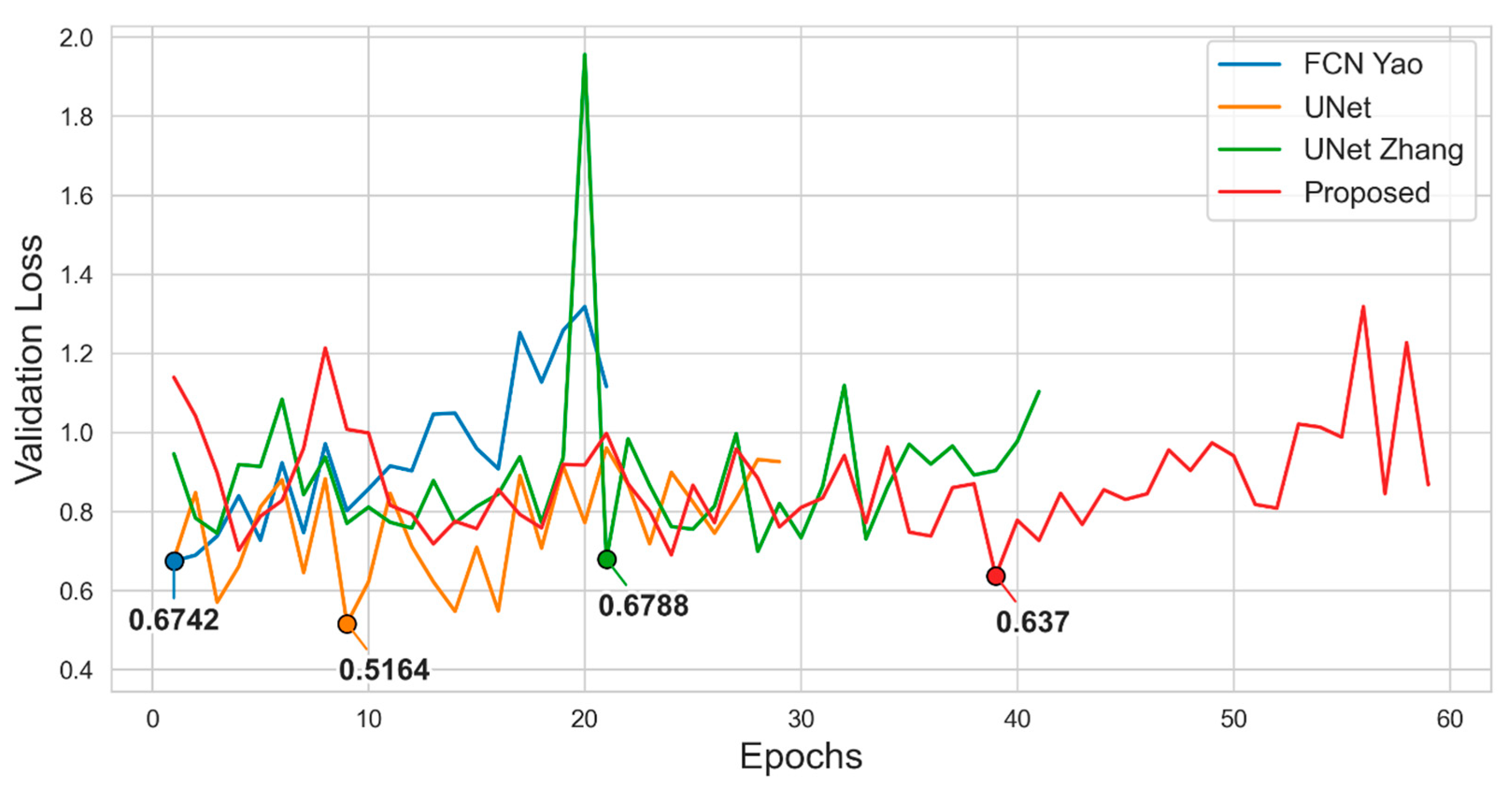
Figure 13 illustrates the change in the validation loss for each model on the PAMAP2 dataset. The proposed model had the second-lowest validation loss of 0.637, and all models exhibited large oscillations and unstable convergence. However, the proposed model achieved the best performance across all metrics, with an accuracy of 86.59%, macro F1-score of 0.847, and weighted F1-score of 0.869.

In terms of computational efficiency, the proposed model yielded the lowest GFLOPs value of 0.034. In contrast, FCN Yao, UNet, and UNet Zhang recorded values of 0.435, 0.081, and 0.173, respectively. Notably, the inference time for the proposed model was 6.6467 s, which is comparable to the inference times of the comparison models. This demonstrates that the dramatic reduction in model size and complexity was achieved without sacrificing inference speed.

The PAMAP2 dataset exhibits a class imbalance, as shown in Figure 14. Owing to subject-based partitioning, there was also a difference in distribution between the validation and test sets; for example, ironing was 12.48% in the validation set and 15.11% in the test set, a difference of approximately 2.63%. With such class imbalance, cross-entropy loss is sensitive to prediction errors in a small number of classes but can be reflected to a limited extent in classification-based metrics, such as accuracy or F1-score [41].

A more fundamental reason for this is that the pattern of misclassification between similar activities, such as Nordic walking and ironing, varies across models. Such confusion between similar classes is sensitive to validation loss; however, its impact on the overall classification performance may be relatively modest.

In conclusion, PAMAP2 is a challenging dataset for classification because of its class imbalance and similar behavior. Nevertheless, the proposed model did not achieve the lowest validation loss but outperformed the baseline model across all metrics.

4.3. Results of WISDM Dataset

Table 5. Performance of the different models on the WISDM dataset.

Model	Accuracy	Macro Averaged F1-Score	Weighted Average F1-Score	Trainable Parameters	GFLOPs	Inference Time
FCN Yao	0.8752	0.8476	0.8783	47,142	0.063	10.7263
UNet	0.9502	0.922	0.9501	2,711,110	0.14	10.7456
UNet Zhang	0.9422	0.9108	0.942	10,497,126	0.301	10.5784
Proposed	0.9456	0.9228	0.946	1,155,430	0.058	10.6067

presents a quantitative performance comparison of the four models on the WISDM dataset. The proposed model achieved a macro F1-score that is 0.06% higher than that of UNet; however, accuracy and weighted F1-score are 0.46% and 0.41% lower, respectively. However, the number of parameters in the proposed model is approximately 42.6% that of UNet, which indicates that the performance degradation is not significant despite its light weight.

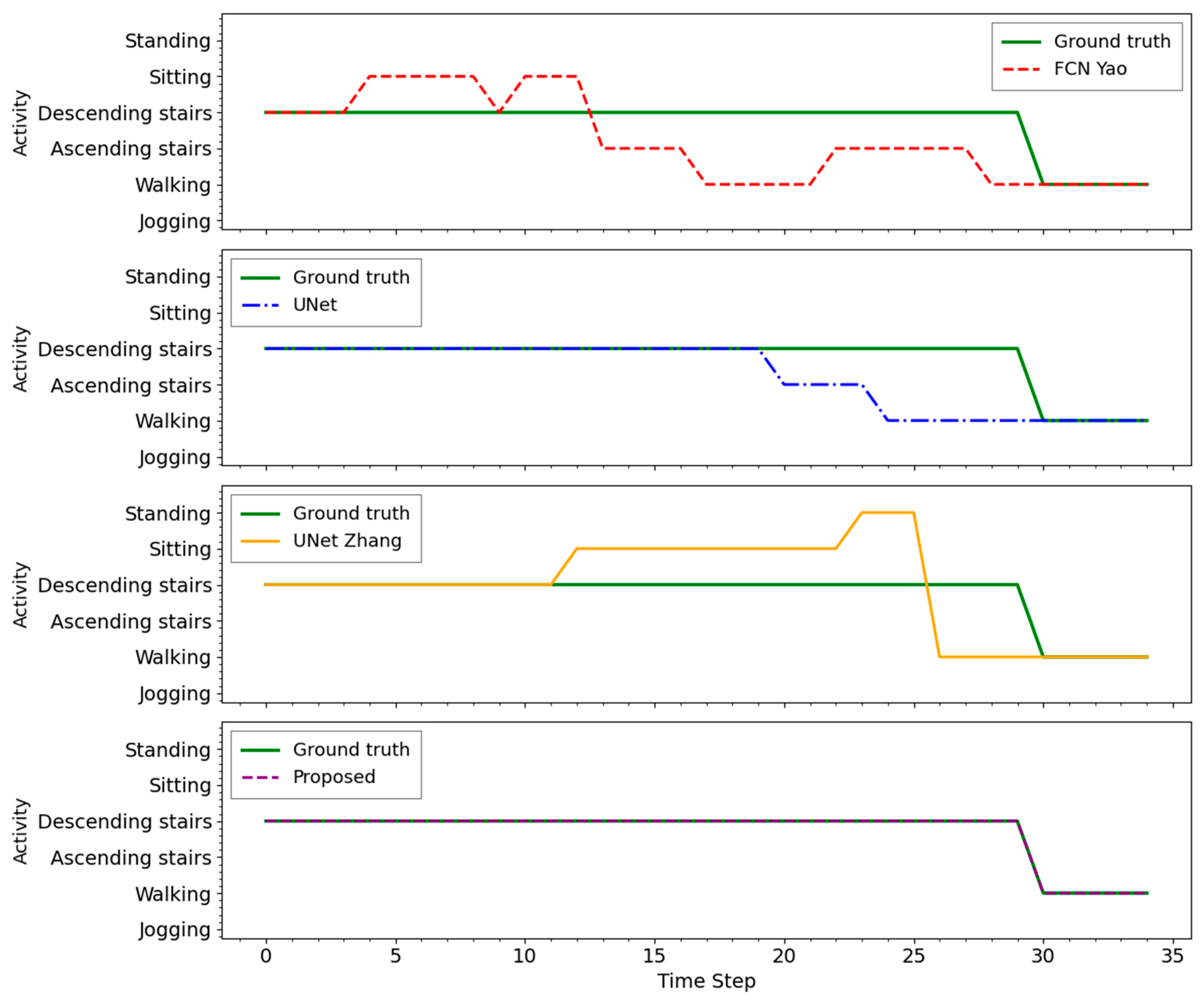
As shown in the dense prediction example in Figure 15, which corresponds to a sample from subject 31 in the test dataset, FCN Yao exhibited the most diverse misclassifications, including incorrectly predicting “Descending stairs” as “Sitting.” UNet Zhang also showed notable (albeit lesser) errors regarding this activity. Although UNet achieved slightly better performance than the proposed model in the overall results table, the dense prediction plot reveals that it still made occasional errors around activity transition points, particularly between “Ascending stairs” and “Walking.” In contrast, the proposed model maintained stable predictions across most segments in the example sequence.

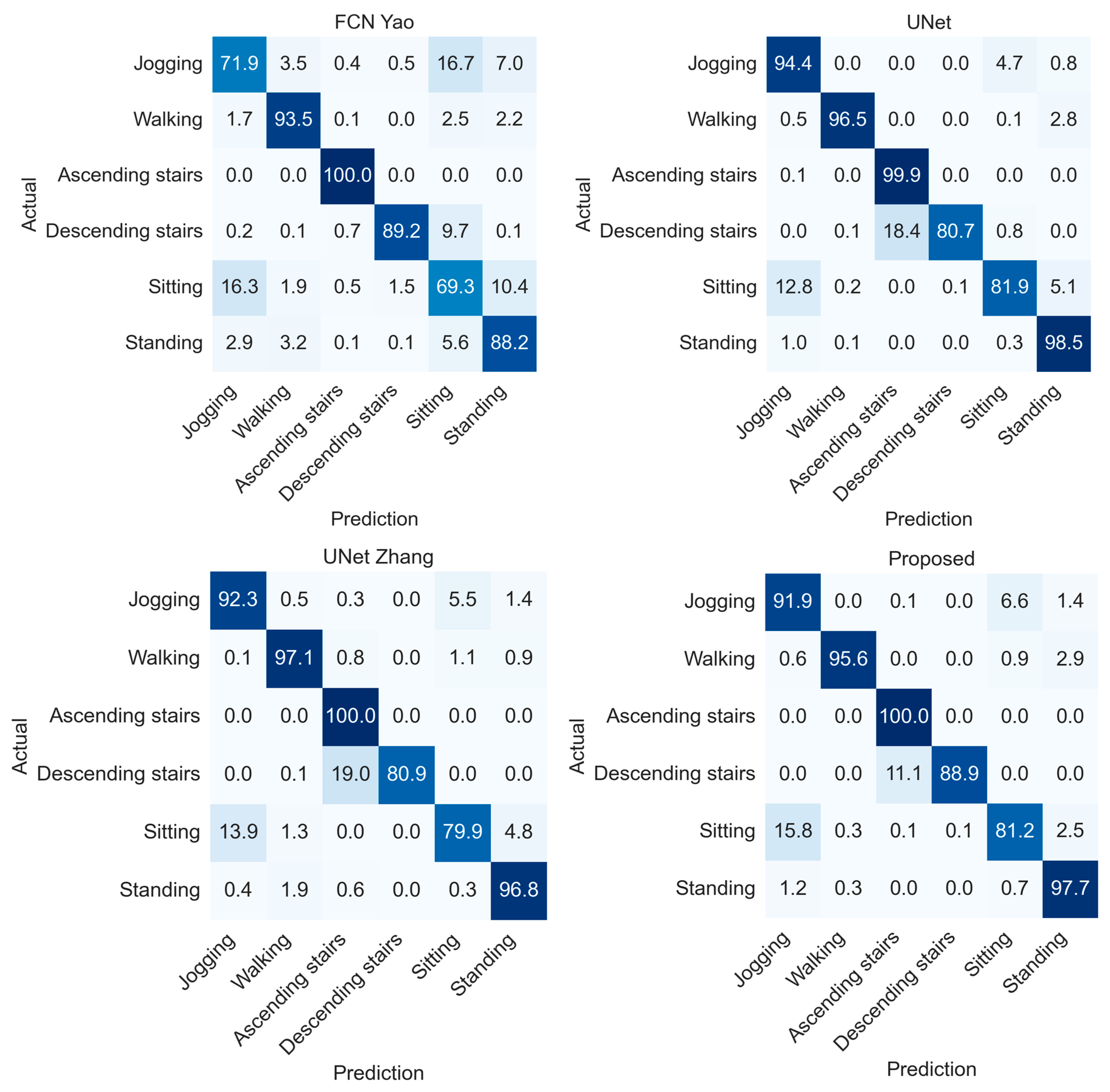
The confusion matrix in Figure 16 shows that misclassifications were concentrated in the “Descending stairs” and “Sitting” activities. “Descending stairs” was misclassified as “Ascending stairs” in most models, which is likely due to the similar movement patterns between walking up and down stairs. FCN Yao’s classification of “Descending stairs” as “Sitting” was found to be inaccurate by 9.7%.

“Sitting” was frequently confused with “Standing” (10.4%) and “Jogging” (16.3%) by the FCN Yao model, and other models exhibited similar trends. The proposed model was relatively stable, classifying “Sitting” with 81.2% accuracy, but misclassifying as “Jogging” in 15.8% of cases. This suggests a limitation in distinguishing static activities with few upper-body movements.

UNet Zhang achieved an accuracy of 0.964 in the original study; however, a randomized split method that mixed data across subjects was employed. As highlighted earlier, random partitioning can lead to an overestimation of the model performance owing to duplication of the same subject data in the training, validation, and test sets. In this study, we applied a subject-independent split, which generally yields lower performance than random splits [42,43]. Under the same conditions, UNet Zhang achieved an accuracy of 0.9422, whereas our proposed model achieved a higher value of 0.9456. In addition, the proposed model performed well across key metrics while requiring approximately 11% fewer parameters.

Similarly, the proposed model demonstrated the lowest computational load among all models, with a GFLOPs value of 0.058, compared to 0.063 for FCN Yao, 0.14 for UNet, and 0.301 for UNet Zhang. Moreover, the inference time, 10.6067 s, was essentially equivalent to those of the baseline models, confirming that the model’s compactness and computational efficiency were achieved without any noteworthy increase in inference latency.

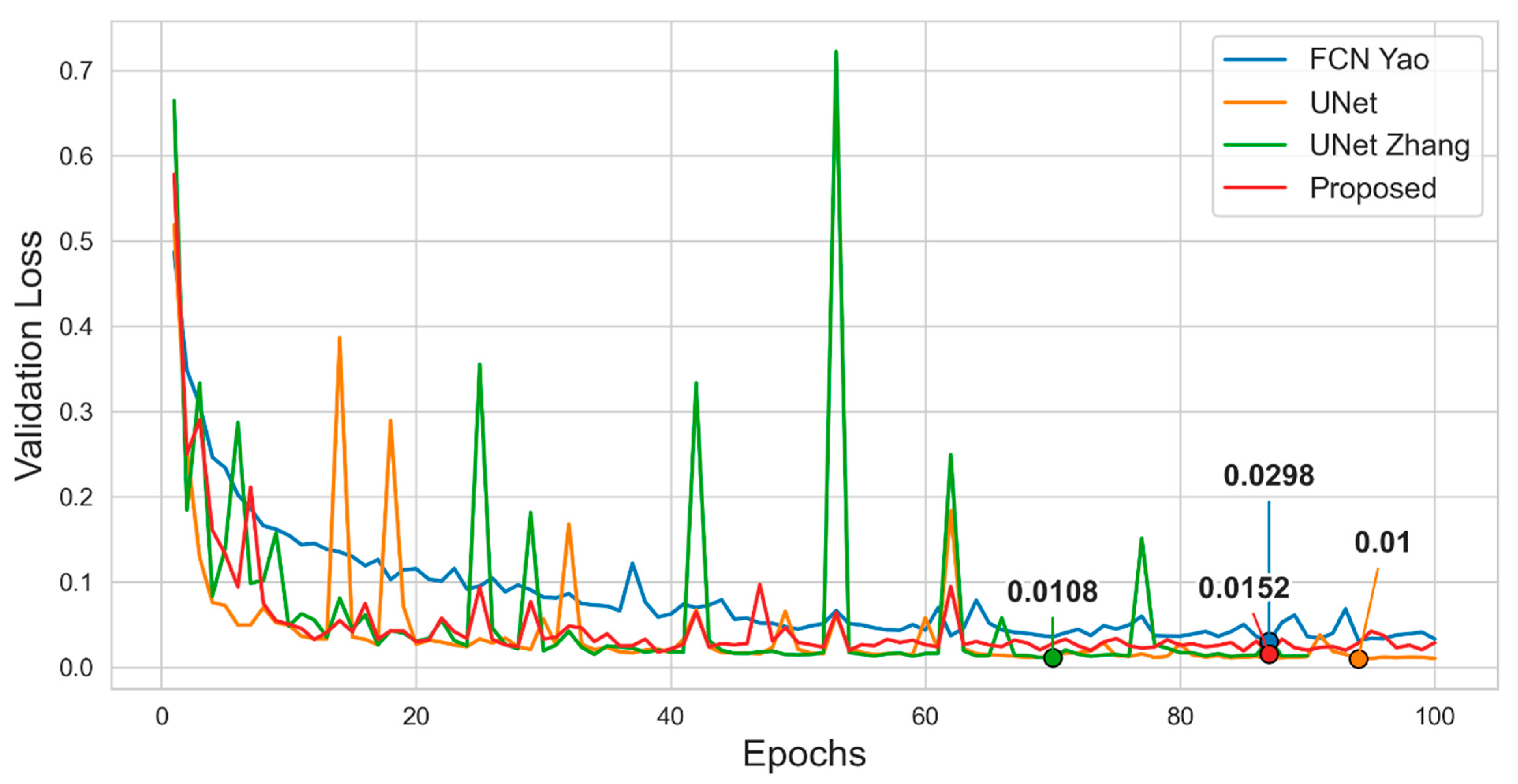
Figure 17 shows the change in validation loss for each model on the WISDM dataset. All four models exhibited an overall decreasing trend; however, UNet and UNet Zhang exhibited unstable behaviors with large fluctuations in some epochs. The validation loss was the lowest for UNet at 0.01, whereas the proposed model had a value of 0.0152. In terms of performance metrics, UNet had the highest values most of the time, but the proposed model had slightly higher values for macro F1-score.

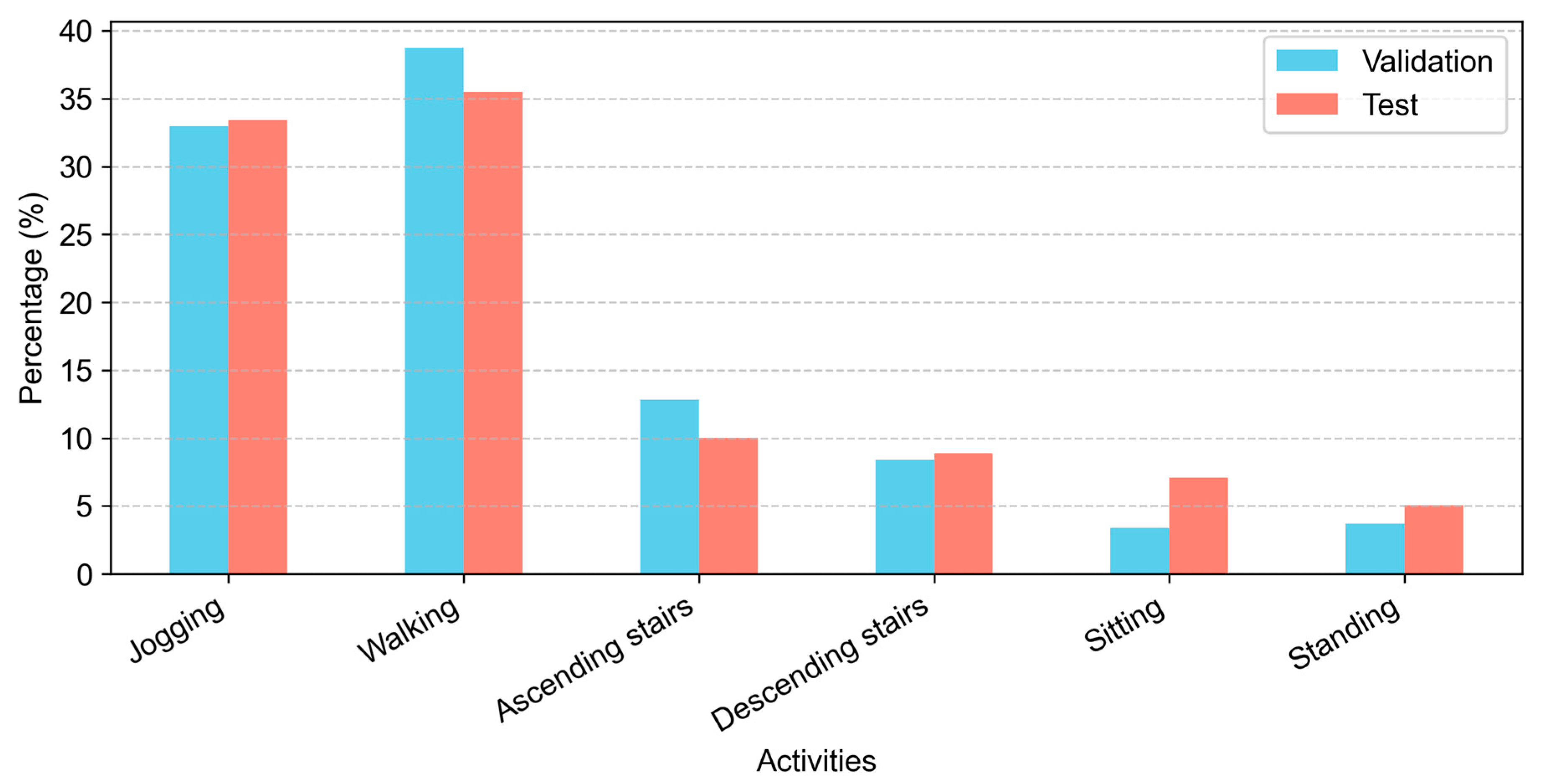
A key feature of the WISDM experiments was that the validation set consisted of random samples from the training data. While the validation set had a class distribution similar to that of the training set, the test set had a different distribution owing to subject-based partitioning. As illustrated in Figure 18, most activities had similar distributions, but sitting exhibited a difference of 3.69%, with 3.39% in the validation set and 7.08% in the test set.

This difference in the distribution of minority classes leads to poor prediction performance. According to the confusion matrix, sitting is frequently misclassified as jogging or standing in all models, which is interpreted as a result of not learning enough features of this behavior owing to the low proportion of the sitting class in the validation set.

In conclusion, the proposed model slightly trails UNet in terms of validation loss, accuracy, and weighted F1-score, but outperforms it on macro F1-score. The proposed model was approximately 42.6% as efficient as UNet in terms of the number of parameters. This demonstrates that the proposed model performs competitively even under unbalanced data and real-world conditions, making it suitable for practical HAR applications.

4.4. Ablation Study

4.4.1. Initial Convolution Configuration

To evaluate the impact of the initial structural settings of the model on the overall performance, we analyzed the differences in performance based on the initial convolutional layer and classifier combination. The feature extraction method in the input and output layer configurations affects the representation ability of the overall structure, which is more important for depthwise separable convolution-based structures.

The PAMAP2 dataset was used in this experiment. PAMAP2 has the largest number of sensors and a strong class imbalance among the compared datasets. Therefore, it is appropriate to compare the impact of input structure differences on the performance, as the complexity of the input time series is high and the initial convolution settings greatly influence the quality of the extracted feature representation.

The initial structures were compared in four ways, as listed in

Table 6. Performance comparison of initial convolution configurations.

Kernel Size	Classifier	Accuracy	Macro Averaged F1-Score	Weighted Average F1-Score
(1, 3)	Conv2d	0.7696	0.7342	0.7551
(1, 3)	Dense	0.76	0.7227	0.7377
(1, 5)	Conv2d	0.7918	0.762	0.7792
(1, 5)	Dense	0.7534	0.7188	0.7358

. The initial convolution kernel sizes were set to (1 × 3) and (1 × 5), and conv2d and dense layers were applied to the classifier. The experimental results showed that the structure combining the (1 × 5) kernel and conv2d classifier demonstrated the highest performance for all major indicators, and this combination was adopted as the final structure.

4.4.2. UNet Block Depth Analysis

In time-series data, the depth of the UNet structure is directly related to the range of temporal context that the model can capture. Generally, as the depth increases, a wider receptive field is secured, enabling the learning of complex temporal patterns. However, this also results in increased computational complexity and the risk of overfitting. Therefore, model depth is a structural hyperparameter that significantly influences performance, and determining an appropriate balance is essential.

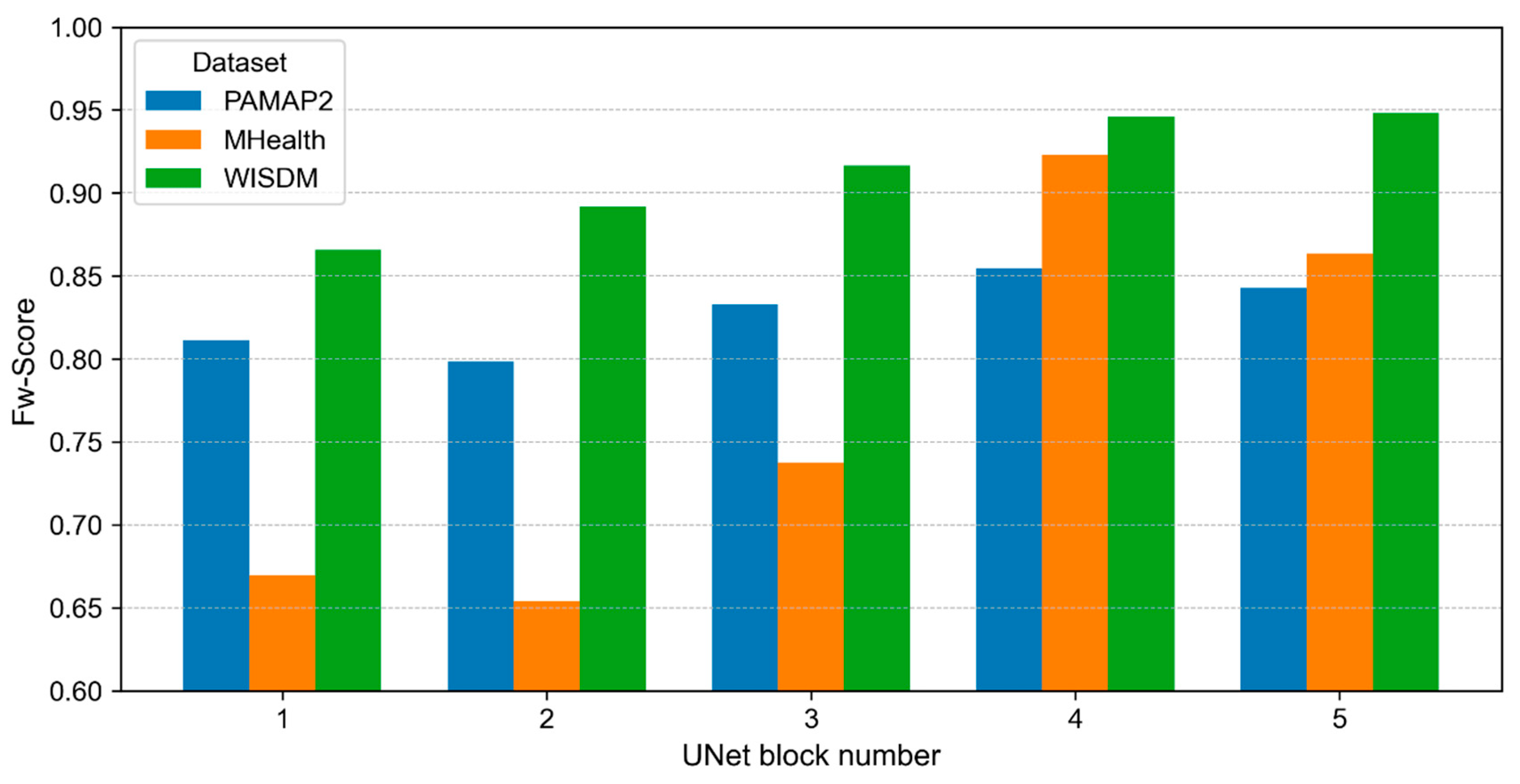
The results of the experiments conducted by varying the number of encoder and decoder blocks from one to five are shown in Figure 19. Across all three datasets, an overall improvement in performance was observed with increasing depth, with the highest weighted F1-score recorded at a depth of four. The WISDM and PAMAP2 datasets exhibited performance plateaus or slight declines after a depth of four, whereas the MHEALTH dataset exhibited a noticeable performance drop at a depth of five. This suggests that excessive depth may compromise learning stability or induce overfitting. Consequently, depth four was adopted as the optimal depth for the proposed model because it demonstrated the most stable and balanced performance across all three datasets.

5. Discussion

The depthwise separable convolution-based UNet structure proposed in this study has demonstrated excellent results in the timestep-by-timestep activity prediction performance of sensor data while significantly reducing the number of parameters and computations. Despite being lightweight, the best prediction performance was obtained for repetitive activities with clear signal changes, such as climbing stairs and jogging, in the MHEALTH dataset.

However, the proposed model struggled with activities with a small number of samples, such as jumping forward and backward in the MHEALTH dataset and sitting and standing in the WISDM dataset, and daily activities with a mix of similar behaviors, such as walking, Nordic walking, and cycling in the PAMAP2 dataset, as did the comparison models. Owing to the nature of the activity composition and distribution in each dataset, misclassification between similar activities and minority classifications remains a major challenge; however, we found the models to be robust to dynamic activity recognition.

In terms of the experimental design, we adopted a method of dividing the dataset into training, validation, and test sets based on the subjects to perform evaluations similar to those in actual environments. This allowed us to verify model performance under stricter conditions than those of the conventional random division method. In particular, unlike in laboratory environments, sensor data collected in uncontrolled, out-of-lab environments such as that in MHEALTH are exposed to various noises, outliers, and sensor errors [33]. Nevertheless, the proposed model performed well across different sensor platforms, individual subject performance characteristics, and complex physical activity recognition.

These results are significant because they demonstrate increased potential for real-world sensor-based HAR applications, particularly for wearable lower-limb exoskeleton robots used for rehabilitation and mobility assistance [44]. Such devices require models that maintain high recognition accuracy under noisy, uncontrolled conditions while operating with minimal computational resources to enable prolonged on-device processing. The proposed lightweight architecture meets these requirements and could support applications for individuals with neuromuscular impairments [45] or lower-limb amputations [46] to overcome mobility limitations and regain physical independence.

However, several limitations should be acknowledged. Inter-user variability—stemming from differences in gait patterns, movement intensity, and sensor-wearing habits—can create domain shifts between training and test sets, potentially limiting model generalizability to user groups that are not well represented in the training data. In addition, environmental factors such as spurious spikes, electronic noise, loose sensor attachment, or prolonged monitoring may cause performance fluctuations and potential misclassifications between similar activities. Addressing these issues may require robust preprocessing, adaptive learning strategies, or personalized calibration to enable reliable real-world deployment.

In summary, the proposed depthwise separable convolution-based UNet maintained frame-level prediction performance while significantly reducing the number of parameters and computational complexity compared to conventional UNet-based models. This performance advantage was consistently observed for dynamic activities or repetitive movements with significant signal variations, as demonstrated across the MHEALTH, PAMAP2, and WISDM datasets. The limitations of static activities with similar signal patterns or blurred boundaries remain, suggesting the need for further structural refinement and dataset-specific optimization.

The limitations of this study are as follows: Although we conducted an ablation study to design the structure of the proposed model, we could not fully optimize the window size and learning parameters for each model and dataset owing to time and resource limitations. In addition, more rigorous validation procedures such as k-fold cross-validation or the leave-one-subject-out (LOSO) method are needed in future studies to confirm the stability and generalizability of the results. However, owing to limited computational resources and the considerable training time required to evaluate each model across all subjects, we report single-run performance in this study.

Moreover, we employed conventional classification metrics (accuracy and F1-score) following the evaluation approach used in previous dense labeling studies [13]. However, specialized metrics for dense prediction tasks such as the error division diagram (EDD), 2-class segment error table (2SET) [47], and segmental F1-score [48] would provide a more accurate assessment of temporal segmentation performance and should be incorporated in future studies.

Furthermore, future work should include comprehensive comparative experiments with recent state-of-the-art models designed for dense prediction tasks, including transformer-based approaches such as self-attention-based BiLSTM models [25] and temporal action segmentation models like OnlineTAS [26].

6. Conclusions

In this study, we propose a lightweight model that applies depthwise separable convolution to a standard UNet structure and validated its performance on representative HAR sensor datasets: MHEALTH, PAMAP2, and WISDM. All experiments were conducted using subject-independent segmentation to evaluate the performance under stringent conditions.

The experimental results indicated that, when evaluated on the MHEALTH dataset, which was collected in an uncontrolled environment, the proposed model demonstrated the most significant performance improvement over the baseline model across all performance metrics, with up to a 10.21% increase in accuracy. On the PAMAP2 dataset, the proposed model exhibited the best accuracy, with a minimum difference of 1.8% and a maximum difference of 4.5%. On the WISDM dataset, the proposed model performed competitively with the best-performing model, UNet, within 0.5%. In the comparison with UNet Zhang, the proposed model achieved superior performance in subject-independent segmentation with 89% fewer parameters. This suggests that the lightweight design of the proposed model can achieve satisfactory results in real-world settings.

This study focused on the lightweight and efficient verification of the depthwise separable convolution-based UNet structure and compared it with representative FCN- and UNet-based dense labeling models. An in-depth comparative analysis using state-of-the-art models is planned for future work. In the future, we will conduct further experiments across different environments and datasets to analyze the generalization performance and practical applicability of the proposed model. In addition, to further validate the practical utility of our approach, we plan to investigate the usability and resource efficiency of the proposed model on actual edge devices, such as smartwatches and smartphones, in future work.