Article

Machine Learning-Based Fracture Failure Analysis and Structural Optimization of Adhesive Joints

1
Department of Engineering Mechanics, College of Pipeline and Civil Engineering, China University of Petroleum, Qingdao 266580, China
2
Engineering Mechanics, College of Science, National University of Defense Technology, Changsha 410073, China
3
Wolfson School of Mechanical, Electrical and Manufacturing Engineering, Loughborough University, Loughborough LE11 3TU, Leicestershire, UK
*
Author to whom correspondence should be addressed.
Appl. Sci. 2025, 15(16), 9041; https://doi.org/10.3390/app15169041
Submission received: 25 July 2025 / Revised: 13 August 2025 / Accepted: 14 August 2025 / Published: 15 August 2025
(This article belongs to the Special Issue New Sciences and Technologies in Composite Materials)

Abstract

The growing use of composites in automotive and aerospace fields highlights the need for effective joining of dissimilar materials. Adhesive bonding offers significant advantages over traditional methods. Therefore, comprehensively exploring the relationship between multiple design variables and joint strength, and subsequently achieving accurate prediction of joint strength based on this understanding, is essential for enhancing the effectiveness and efficiency of adhesive joint structural optimization. However, the joint—the critical yet weakest part—has strength governed by complex structural variables that are not fully understood, limiting optimization potential. Based on the effectiveness of finite element simulation in tensile fracture mechanics, this study developed a deep neural network (DNN). Combining the DNN model with a genetic algorithm (GA), both single-objective and multi-objective optimization were conducted. The single-objective optimization focused solely on maximizing joint strength, while the multi-objective GA further quantified the Pareto optimal trade-offs between joint strength and bond area, identifying compromise solutions. The effectiveness of the optimized parameters was validated, demonstrating higher efficiency and accuracy compared to traditional optimization methods such as response surface methodology (RSM). This integrated approach provides a robust framework for predicting joint strength and achieving effective optimization of bonded structures.

1. Introduction

In automotive [1], aerospace [2], and related engineering fields, joining structural components is essential. While bolted connections and adhesive bonding are both widely used, they present distinct advantages and limitations. Bolted connections facilitate disassembly and recycling but inherently create stress concentrations at fastener interfaces and require drilled holes in adherends, thereby compromising structural integrity and potentially leading to premature failure. Adhesive bonding, by contrast, offers several key benefits: it maintains adherend continuity, enables lightweight design, and provides excellent vibration damping and impact resistance due to the adhesive layer’s low elastic modulus and viscoelastic characteristics. These properties make adhesive bonding particularly suitable for vibration-sensitive applications in aerospace and automotive structures. The primary failure modes of bonded joints are cohesive failure within the adhesive layer or interfacial (adhesive) failure at the bond interfaces. Accurately predicting stress distributions in these joints remains challenging, as eccentric loading typically induces complex peel and shear stresses, resulting in bond line deflections. Addressing this complexity through improved modeling has been an ongoing research focus for decades.
Adhesive joints—the connection points in bonded structures—often represent the most critical yet vulnerable components within composite assemblies. On one hand, the strength of these joints directly dictates the overall load-bearing capacity of composite structures. On the other hand, over half of all failures in bonded composite structures originate at these connection points. Consequently, the design of adhesive joints constitutes a paramount consideration in bonding processes, with joint strength serving as the primary metric for evaluating joint performance and design quality. Current research on adhesive joint strength primarily focuses on two key aspects: predicting joint stresses and analyzing crack initiation and propagation as the adhesive joint failure.
Building upon the earlier model by Goland and Reissner [3], subsequent developments accounted for the bending effects in adhesive joints and the resulting influence of peeling stresses within the adhesive layer, leading to the derivation of more precise formulas for adhesive stress distribution. Hart-Smith [4] modeled the adhesive as an ideal elastic–plastic material, considering only its shear deformation. Based on this assumption, he derived a series of simplified analytical models. Zhao [5,6] derived the stress distribution at the adhesive joint from the perspective of elasticity mechanics, and Cheng [7,8] creatively derived the theoretical formulas for asymmetric adhesive joints, representing a significant advancement in the theoretical solutions for adhesive joint structures. Based on experimental data and Weibull statistical analysis, Arenas [9] investigated the influence of adhesive layer thickness on the mechanical performance of single-lap joints. Their study aimed to determine the ideal adhesive thickness for achieving optimal reliability and joint performance. It was found that a critical adhesive thickness threshold exists; below this value, joint strength increases with greater adhesive thickness, whereas exceeding it results in progressively decreased strength. Apart from the size of the structure, the adhesive is also a factor closely related to the strength of the joint. Öz and Özer [10] compared the effects of three adhesives with varying strength and fracture toughness—AV138, Araldite 2015, and DP-8005—as well as their mixtures in different proportions, on the strength and fracture patterns of single-lap joints during tensile testing. Their results demonstrated that placing rigid adhesive at the center of the bonding area while using toughened adhesive at both ends significantly improves stress distribution, thereby enhancing joint strength. While experimental and analytical methods offer distinct advantages, both have limitations. Advances in finite element methods (FEMs) have enabled detailed numerical models of adhesive joints. Researchers now use these to study bonded structures under various parameters. Bendemra [11] used 2D FE models to analyze scarf/stepped-lap joints, revealing that adhesive layer stress is highly sensitive to ply thickness/stacking sequence (especially 0° ply position). Building on this, Sulu [12] conducted 3D simulations in ANSYS examining single-/double-lap joints, determining optimal parameters and connection methods.
Research on fracture in adhesive joints still primarily relies on finite element simulation methods, such as the cohesive zone model (CZM) and the extended finite element method (XFEM). In contrast, Gong [13] proposed a novel numerical simulation strategy for reinforced concrete (RC) structures based on a rigid-body-spring model. According to this strategy, concrete is discretized into a series of irregular rigid blocks according to a Voronoi diagram, interconnected by interface springs. A damage evolution model for concrete, based on a separation criterion, describes the degradation process of these interface springs between adjacent blocks. This approach significantly improves prediction accuracy. In recent years, the Discrete Element Method (DEM) has been extensively applied to crack simulation. Building on this, Xu [14]’s study employs a DEM simulation model to investigate the micromechanical properties of ballast beds under fastener failure conditions, accurately capturing the actual geometry of ballast particles. Cao [15,16] conducted separate investigations into the effects of distinct linear defects and high-strength submicron precipitates on crack initiation and propagation.
As research advances, the recognition has grown that the underlying mechanisms governing composite behavior are highly complex. Concurrently, the rise of artificial intelligence has enabled a novel approach: leveraging machine learning techniques [17] applied to both numerical simulation data and traditional experimental data to analyze the collective impact of multiple variables on overall composite performance. Wang and Zhang [18,19] significantly reduced data requirements by combining machine learning with molecular dynamics in the field of femtosecond laser applications. Mashrei [20] developed a backpropagation neural network model that accounts for adherend width and length effects to predict bond strength in FRP-to-concrete joints. This approach was applied to predict the strength of adhesively bonded single-lap composite joints with varying overlap lengths and adhesive thicknesses [21]. The results demonstrated that the artificial neural network (ANN) method achieved significantly higher computational efficiency compared to analytical and multiple linear regression models. However, for image-related problems, the advantages of Convolutional Neural Networks (CNNs) become highly pronounced. Wang [22] proposed integrating CNNs to predict wrinkling defects in tube bending, significantly enhancing efficiency.
Beyond ANN and CNN models, the genetic algorithm (GA)—an optimization technique simulating natural selection—has emerged as a powerful tool. Initially applied to structural mechanics, researchers utilized GAs to calculate load capacities of steel beams [23], predict distortional buckling stress in steel sections [24], and characterize the mechanical properties of rocks [25]. Recent advances have extended genetic algorithm (GA) [26] applications to adhesive joint optimization. Al-Mosawe [27] successfully implemented GAs to predict bond strength in CFRP-steel double-strap joints under varying loading rates. However, their analysis considered only a limited set of continuous variables: bond length and loading rate.
This research presents a comprehensive investigation of composite single-lap joints through an integrated computational approach. This study establishes parameterized finite element models to characterize the tensile fracture behavior and failure mechanisms of the joints, while employing deep neural networks to explore the correlation between multiple design variables and joint strength for accurate failure load prediction. Response surface methodology is applied to analyze the influence mechanisms of structural variables on joint performance, with comparative assessments against alternative response surface models. Furthermore, the research implements genetic algorithm-based single- and multi-objective optimization to determine optimal design parameters, with validation conducted through systematic comparison with ANSYS 19.2 native optimization tools to evaluate the proposed methodology’s effectiveness.

2. Analysis of the Tensile Fracture Failure of Single-Lap Joints

2.1. Adhesive Failure Analysis Based on the CZM Cohesion Model

The cohesive zone model (CZM) [28], based on elastic–plastic fracture mechanics, is widely employed to simulate crack propagation in concrete and composite materials. When applied to model damage and fracture failure, CZM requires a predefined crack propagation path. This model simulates macro-crack growth along this path by defining the traction–separation response (stress vs. crack opening displacement) on the predefined path. The fundamental concept of CZM posits the existence of a small cohesive zone ahead of the macro-crack tip. Within this cohesive zone, the stress acting perpendicularly on the crack faces, which tends to open the crack, equals the cohesive strength. Before actual physical crack formation occurs, this region features a subcritical crack opening displacement ω—representing a cohesive crack. The stress across the crack faces is a function of this opening displacement ω, expressed by the relation:
σ = f ω
The energy required for the generation of a new crack surface is called fracture energy, and its expression is
G = σ d w
As illustrated in Figure 1a, during the opening of a cohesive crack, the stress acting across the crack faces initially increases with crack opening displacement (ω). This stress reaches a maximum value, σmax, signifying the onset of damage within the material. Subsequently, if the opening displacement continues to increase, the stress progressively declines. When the stress diminishes to zero, the material experiences complete failure, resulting in full crack formation within the cohesive zone and the emergence of a macro-crack. The energy dissipated during this entire process constitutes the fracture energy G, which corresponds to the area enclosed under the traction–separation curve. Consequently, the cohesive zone model is primarily defined by two key parameters: the cohesive strength, σmax, and the fracture energy, G. These parameters typically require experimental determination. Different shapes of the CZM traction–separation law correspond to distinct damage evolution laws [29,30]. Commonly used laws include the bilinear and exponential forms (Figure 1b,c); however, the specific choice of law generally has a minor influence on the overall fracture energy represented by the curve.
In this model, adhesive tensile fracture involves mixed-mode (I/II) failure. Upon loading, the cohesive element’s two layers of nodes exhibit relative displacements only in the directions parallel to the crack plane (shear sliding, δₛ) and perpendicular to it (normal opening, δₙ). Consequently, tractions develop between the layers: a shear traction, τ, parallel to the crack plane and a normal traction, σ, perpendicular to it. For pure fracture modes, as depicted in Figure 1b, the normal traction, σ, increases linearly with the normal opening displacement, δₙ, until it reaches the interface’s maximum tensile strength, σmax. Subsequent increases in δₙ initiate damage in the cohesive element. For mixed-mode fracture, crack initiation follows specific criteria, such as the Maximum Nominal Stress Criterion and the Quadratic Nominal Stress Criterion, expressed in Equations (3)–(6).
max τ n τ n 0 , τ s τ s 0 , τ t τ t 0 = 1
max δ n δ n 0 , δ s δ s 0 , δ t δ t 0 = 1
τ n τ n 0 2 + τ s τ s 0 2 + τ t τ t 0 2 = 1
δ n δ n 0 2 + δ s δ s 0 2 + δ t δ t 0 2 = 1
Damage evolution is governed by two primary criteria [31]: one based on effective displacement, and the other based on fracture energy. Energy-based laws include the exponential form and the Benzeggagh–Kenane law, as given in Equations (7) and (8).
G n G n C α + G s G s C α + G t G t C α = 1
G n c + G s c G n c G S G T η = G c
where G S = G s + G t G T = G s + G n   G n , G s , G t represent the work of normal stress, the first shear stress, and the second shear stress, respectively. G n c , G s c , G t c are, respectively, expressed as Type I, Type II, and Type III fracture energies. The exponent η represents a parameter in the semi-empirical criterion governing both crack initiation and propagation. Typically, η ranges from 1 to 2. In this study, η = 2 was adopted.

2.2. Finite Element Simulation of the Failure of Single-Lap Joint Due to Tensile Fracture

Modeling and simulation of the single-lap joint were conducted using Ansys Workbench finite element software. This study focuses on the influence of structural design variables on the joint’s tensile fracture strength. Comparative simulations revealed that while the 2D model yields joint strength predictions comparable to the 3D model, it significantly reduces computational time. Consequently, the model neglects the effect of joint width on strength, assuming uniform stress distribution along the width direction. The single-lap joint was thus simplified to a 2D plane strain model and parameterized for analysis.
The model comprises three distinct parts: the upper adherend, the adhesive layer, and the lower adherend. The adhesive layer was partitioned along its middle surface into upper and lower sub-regions. All interfaces between joint components were connected using bonded contact. The boundary conditions for the single-lap joint are illustrated in Figure 2. One end (left end) is fully constrained with fixed supports restricting all translational and rotational degrees of freedom. The opposite end (right end) has fixed constraints applied to translational and rotational movements in both the y- and z-directions. A prescribed displacement of 1.2 mm is applied solely along the x-direction until final tensile failure occurs.
To investigate the influence of structural design variables on joint strength and enable efficient batch sampling for strength calculations, this study established a parameterized 2D finite element model (Figure 2). The four key structural design variables (lap length, upper adherend thickness, lower adherend thickness, and adhesive thickness) were defined as parameters in Design Modeler. Their allowable ranges are documented in Table 1.
The upper and lower adherends of the studied adhesive joint utilize aluminum alloy 6082-T6, a material series widely employed in the automotive industry. This alloy offers excellent corrosion resistance, toughness, notable heat resistance, ease of processing, high recyclability, and energy efficiency. The adhesive used for bonding is Araldite® 2015 [32], a two-component room-temperature-curing structural adhesive. It provides superior bonding strength, durability, and elastic adhesion while maintaining stable performance under diverse environmental conditions. Fundamental material properties and adhesive fracture parameters are detailed in Table 2 and Table 3.

3. The Joint Strength Is Based on Research on Deep Neural Network Machine Learning

3.1. Data Sampling and Preprocessing

To develop an accurate and generalizable surrogate model for predicting the tensile strength of single-lap adhesive joints, a structured dataset was generated through high-fidelity finite element (FE) simulations. Based on the parametric model introduced in Section 2, four key structural design variables were identified as input features: adhesive thickness (t), lap length (L), upper adherend thickness (T1), and lower adherend thickness (T2). Their allowable ranges were defined in accordance with practical engineering constraints and are listed in Table 1.
To ensure uniform coverage of the design space and reduce sampling bias, Latin Hypercube Sampling (LHS) [33] was employed to generate 300 sample points. Each configuration was simulated under tensile loading using the validated FE model to extract the corresponding failure load, which served as the supervised learning target. Prior to training, all input and output variables were normalized using min–max scaling to the range [0, 1], enabling faster convergence and improving numerical stability during model optimization. The dataset was further partitioned using a 3-fold cross-validation scheme to facilitate model robustness evaluation and guard against overfitting.

3.2. Construction and Training of Machine Learning Models

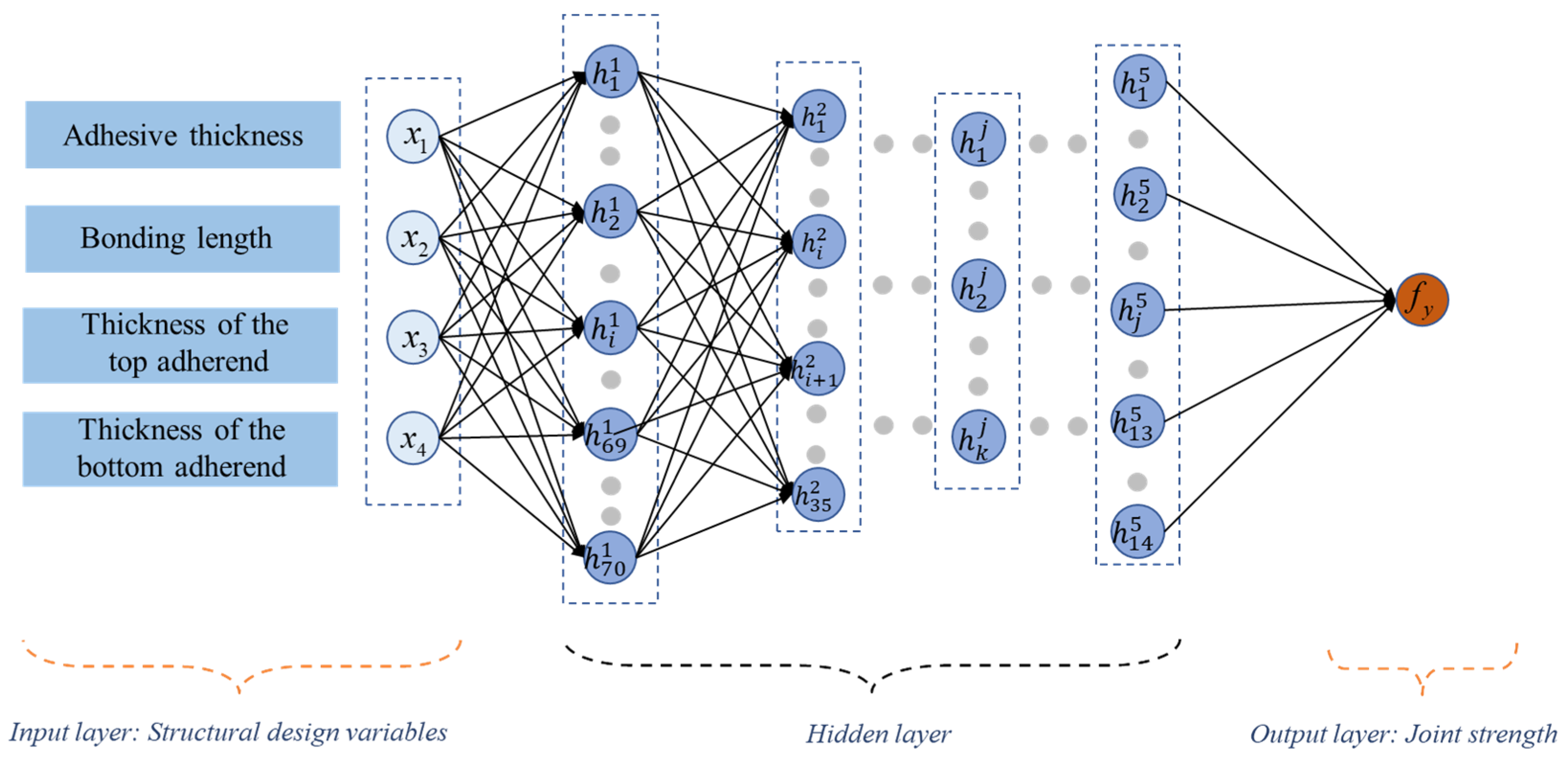
This study employed an artificial neural network (ANN) algorithm to uncover the complex relationships between structural design variables and joint strength. The ANN serves as the foundation for deep neural network (DNN) algorithms. Designed to simulate biological nervous systems, the ANN architecture draws inspiration from biological neurons. Biological neurons receive signals through dendrites and undergo modulation or generate responses based on signal intensity. When the integrated signal strength reaches a threshold, the neuron activates, forming connections with other neurons via synapses to transmit information. In the ANN, the input layer receives various parameters from the training data. These parameters are then transformed and modulated by activation functions within the hidden layers. During this process, each neuron in a hidden layer computes a weighted sum of its inputs, incorporating its specific weights and bias term. This sum is then evaluated by an activation function (often conceptualized as a step function) to determine if it exceeds a threshold. If the threshold is surpassed, the signal is propagated to the next layer. These outputs subsequently serve as inputs for neurons in the following layer.
In this model, we employ an architecture comprising an input layer, five hidden layers with neuron counts decreasing stepwise from 70 to 14, and an output layer. Leaky ReLU activation functions are used for all hidden layers, while a linear function is applied to the final output layer. To mitigate potential overfitting risks arising from arbitrary single splits in the training data workflow, a dropout rate of 0.2 is implemented for each hidden layer. Additionally, training is configured with a batch size of 25 and an early stopping criterion defined at 2000 epochs. When an artificial neural network becomes “deeper” by adding multiple hidden layers, as shown in Figure 3, this network structure is called a deep neural network (DNN). This sequential signal propagation continues layer by layer until the final output layer produces the result.

4. Single-Lap Joint Based on Structural Optimization Design of DNN Model and Genetic Algorithm

4.1. Single-Objective Optimization Research

To maximize the tensile strength of single-lap adhesive joints while avoiding the computational cost of repeated finite element simulations, a structural optimization framework was developed by coupling the trained deep neural network (DNN) surrogate model with a genetic algorithm (GA).
The GA was selected for its global search capability and robustness in navigating nonlinear, multi-dimensional design spaces. The objective function was defined as the maximization of predicted joint strength, subject to the design constraints listed in Table 1. The optimization process was executed using a standard GA implementation with binary tournament selection, simulated binary crossover, and polynomial mutation. The DNN model was embedded within the GA loop to rapidly evaluate fitness across generations, dramatically reducing the need for direct FE computation.
This model was implemented in geatpy using the single-objective optimization problem template. By defining the problem class MyProblem, we configured the specific details of the single-objective optimization problem, encompassing four design parameters: adhesive layer thickness, overlap length, and the thicknesses of the upper and lower adherends. The optimization objective function leverages the predictive relationship between structural design variables and joint strength established by the DNN model in Section 3. This is achieved by decoding the decision variable matrix, applying normalization, and utilizing predictions from the pre-trained machine learning model, followed by denormalization to yield the predicted joint failure load. The algorithm settings included a population size of 6000 individuals, evolved over 234 generations, with mutation and crossover probabilities set to 0.25 and 0.7, respectively.

4.2. Multi-Objective Optimization Research

In practical adhesive joint design processes, the overlap length typically ranges from 10 mm to 30 mm to satisfy requirements for lightweight design and cost efficiency. Within this context, a common design challenge involves maximizing joint strength while minimizing adhesive usage. To address this problem, this section employs a genetic algorithm (GA) to construct a multi-objective optimization model, as defined by Equations (9)–(11). This model aims to simultaneously maximize joint strength and minimize adhesive consumption.
O p t F , S = M a x F M i n S
F = F t , L , T 1 , T 2 = D N N t , L , T 1 , T 2
S = S t , L = t × L
Given that the finite element model is two-dimensional, the adhesive usage is represented by the adhesive area, S (calculated as adhesive thickness multiplied by overlap length). The joint strength function, F, embodies the nonlinear relationship between the design variables and joint strength, as captured by the DNN model established in Section 3. The MOGA was built based on the same DNN model used in the single-objective case, enabling efficient fitness evaluation of thousands of design candidates.
In multi-objective optimization, it is generally impossible to find a single solution that simultaneously optimizes all sub-objectives. Consequently, genetic algorithms (GAs) are widely employed to address such problems due to their exceptional global search capabilities. This approach effectively explores trade-offs between competing objectives, identifying a set of solutions where each represents an optimal compromise between the conflicting goals.
Fifteen superior solutions selected from the Pareto optimal set were ranked using the Technique for Order Preference by Similarity to Ideal Solution (TOPSIS)—a multi-criteria decision analysis method that precisely quantifies differences between alternatives. This involved constructing a decision matrix with the 15 non-dominated solutions, normalizing the matrix to render objective values dimensionally comparable, and applying weights to create a weighted normalized matrix. The positive ideal solution (PIS) and negative ideal solution (NIS) were then identified. Euclidean distances from each solution to both the PIS and NIS were computed, enabling calculation of the relative closeness (RC = Distance to NIS/(Distance to PIS + Distance to NIS)) for each solution. Solutions were finally ranked by their RC values, with the solution exhibiting the highest RC (representing the alternative closest to the PIS and farthest from the NIS) identified as optimal.
The model structure is similar to that described in Section 4.1. However, this formulation incorporates two optimization objectives: maximizing joint strength and minimizing adhesive volume. To align with the algorithm’s maximization framework, the minimization of adhesive volume is implemented by taking its negative value. Other algorithmic parameters include a population size of 1000, evolution over 20 generations, a mutation probability of 0.25, and a crossover probability of 0.7.

5. Results and Discussion

5.1. Verification of Finite Element Results and Accuracy Analysis of ML

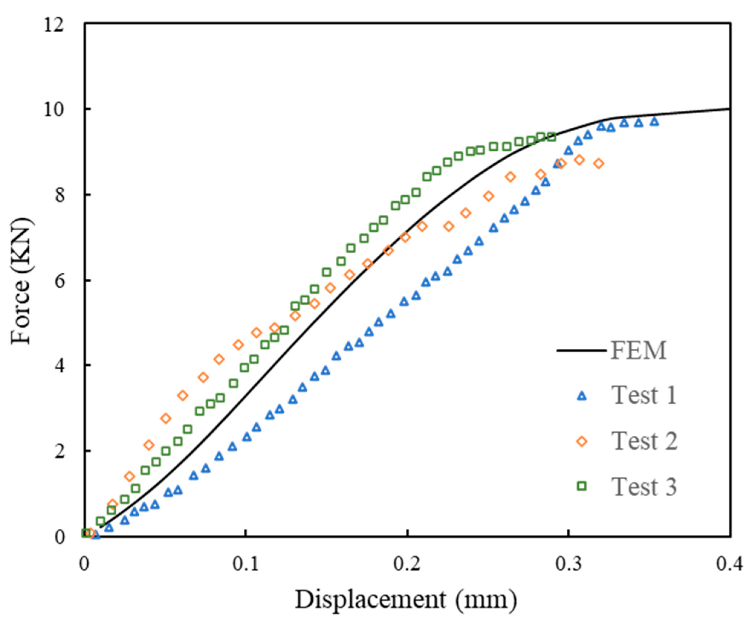
Through the post-processing of the finite element simulation data, the force–displacement curve during the tensile fracture failure of the adhesive joint was plotted (as shown in Figure 4). Comparison with experimental results reveals that the slopes and trends of both curves closely match, validating the accuracy of the finite element simulation.
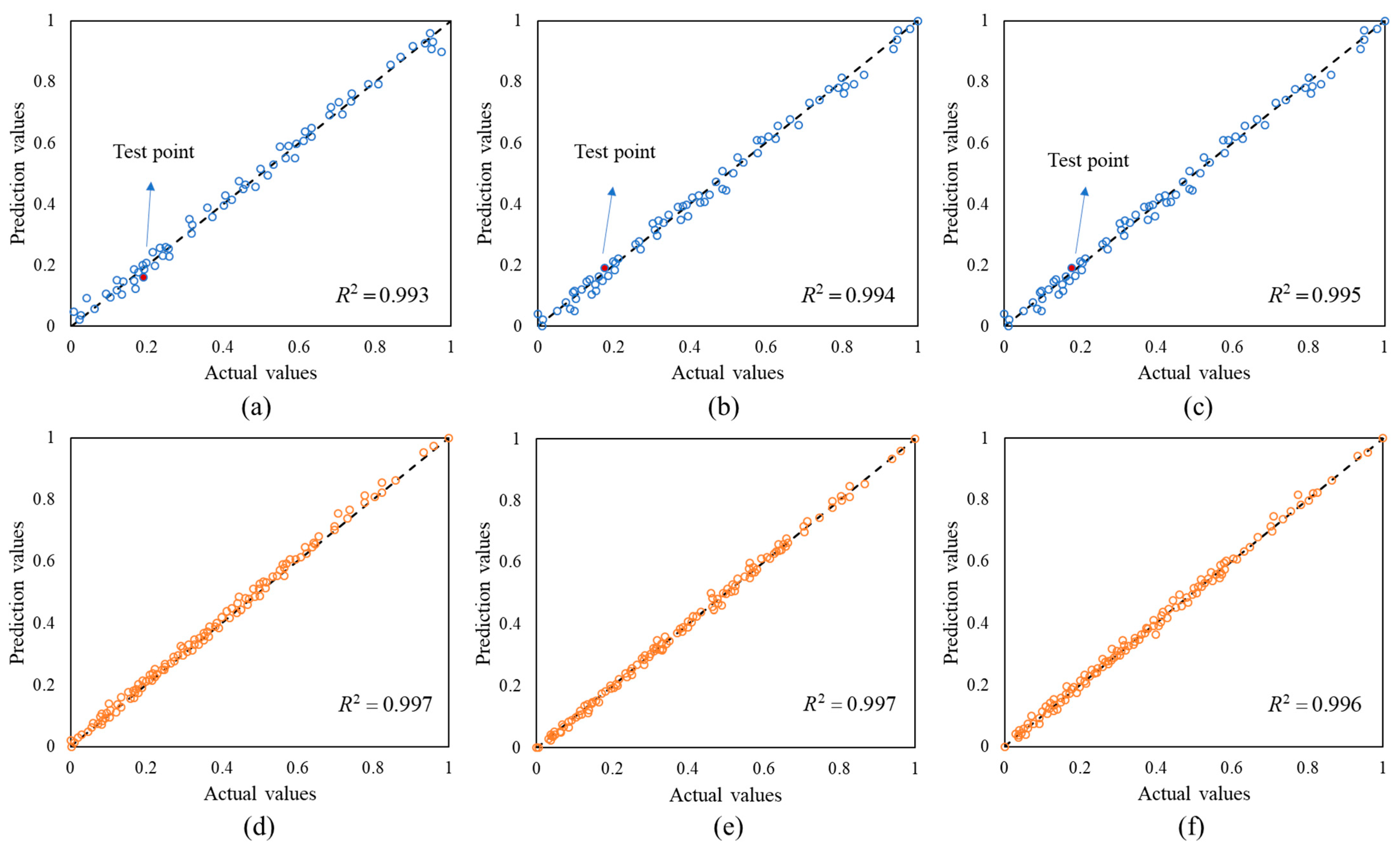
Figure 5 presents the performance of the deep neural network (DNN) model in predicting the tensile strength of single-lap joints using 3-fold cross-validation. Figure 5a–c correspond to the predictions on the training datasets of each fold, while Figure 5d–f display the corresponding test results. The x-axis represents the reference strength values obtained from finite element simulations, and the y-axis denotes the DNN-predicted values. The coefficient of determination (R2) is reported in each subplot to quantitatively assess prediction accuracy.
During training (Figure 5a–c), the DNN model achieves R2 values of 0.991, 0.990, and 0.990, respectively, indicating excellent fitting capability. The predicted values align closely with the reference data across all folds, showing minimal scatter and no apparent signs of overfitting. For the test sets (Figure 5d–f), the model maintains high predictive accuracy, with R2 values of 0.990, 0.988, and 0.988, respectively. The data points are densely distributed along the diagonal reference line, confirming the DNN’s strong generalization performance. The consistency of the R2 values across folds highlights the robustness and stability of the model when exposed to unseen data.

5.2. ML Response Surface Result Analysis

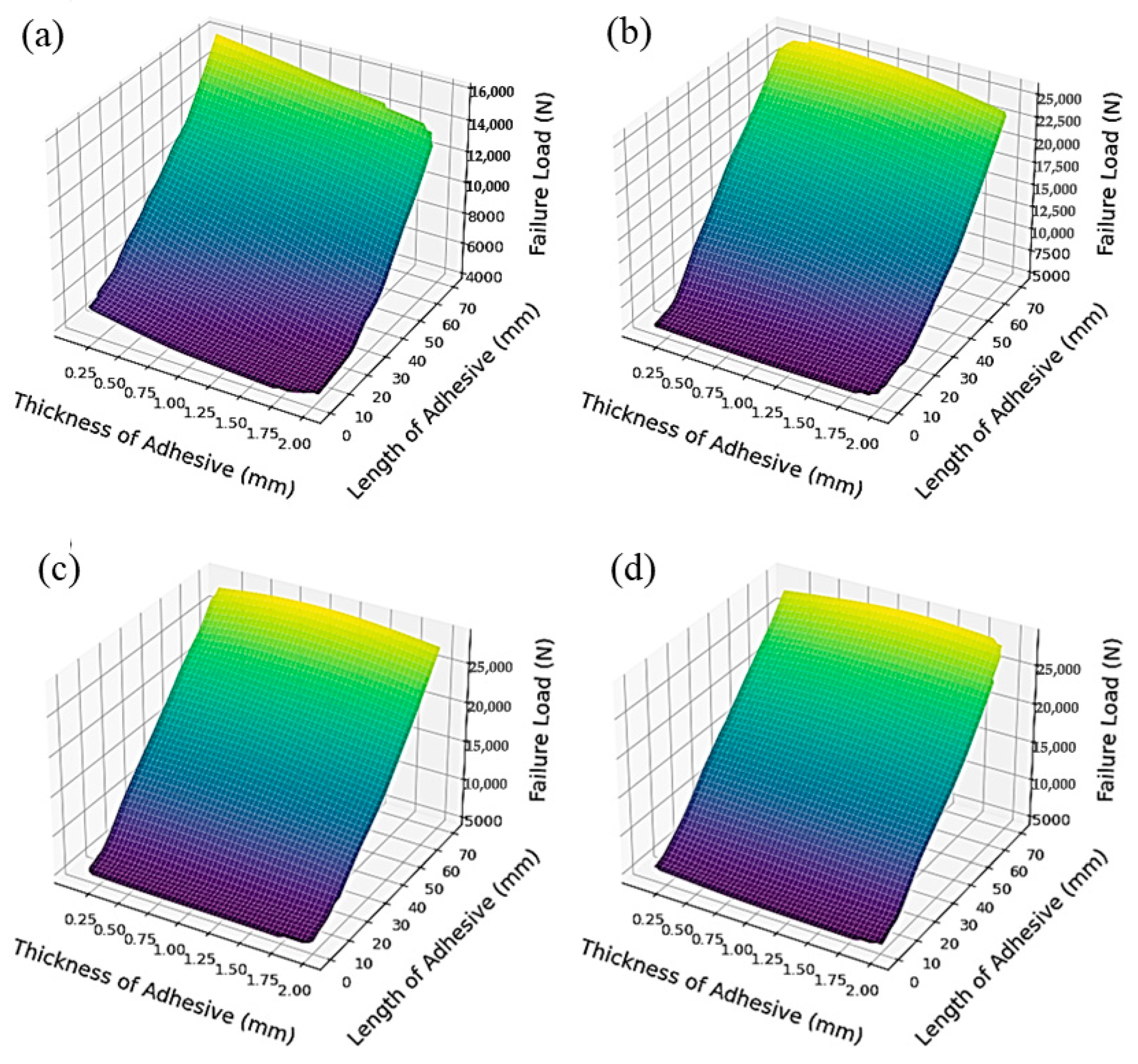
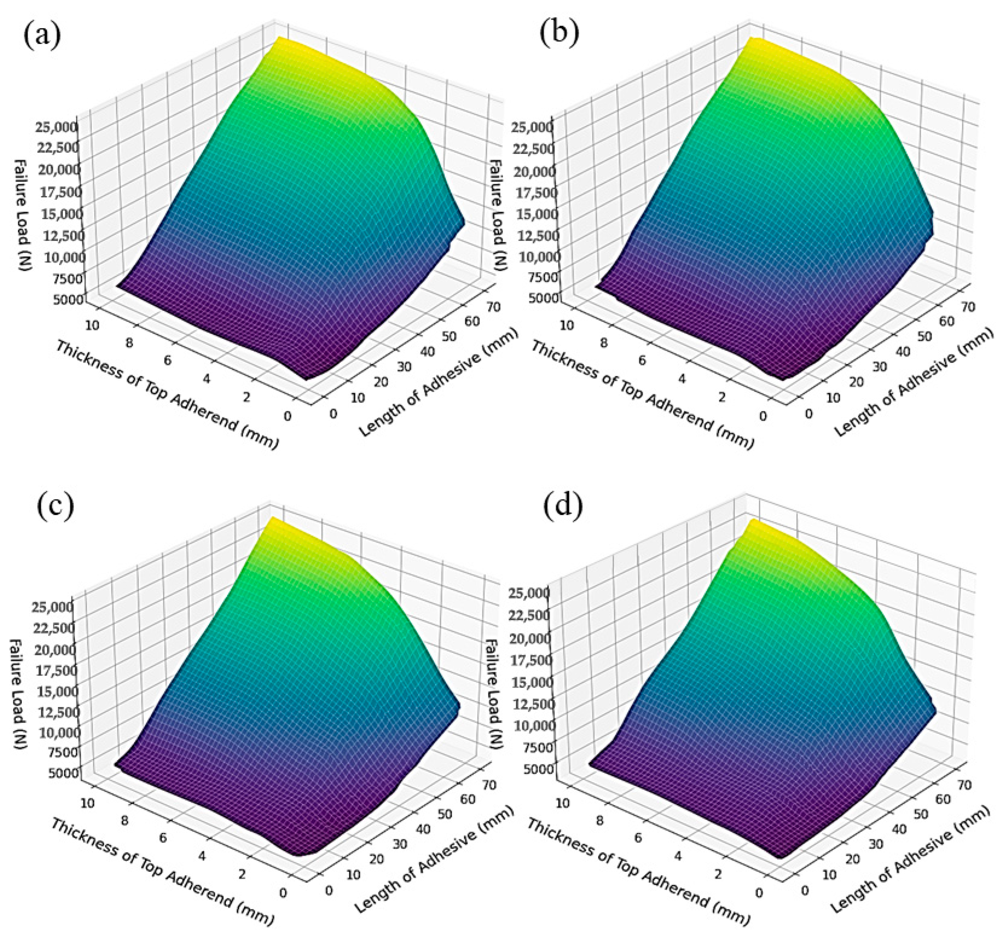
Figure 6 presents the response surface plots of the predicted failure load as a function of adhesive thickness and lap length under varying lower adherend thicknesses (T2 = 1 mm, 4 mm, 7 mm, and 10 mm), as obtained from the trained deep neural network (DNN) model. These surfaces clearly demonstrate the complex, coupled influence of geometric parameters on joint performance. Across all cases, lap length emerges as the most influential factor—longer overlaps consistently lead to higher failure loads due to increased bonded area and enhanced load transfer efficiency. Adhesive thickness exhibits a nonlinear effect: at lower values, increasing thickness significantly improves joint strength by providing greater energy dissipation and deformation capacity; however, beyond a certain threshold, the benefit plateaus or even slightly declines, likely due to stress concentration and reduced stiffness. Notably, as the lower adherend thickness T2 increases from 1 mm to 10 mm, the overall magnitude of the predicted failure load rises substantially, underscoring the critical role of adherend stiffness in reinforcing structural integrity and mitigating peel and shear stresses within the adhesive layer. The curvature and steepness of the response surfaces evolve with T2, reflecting stronger interaction effects at higher thickness levels. These high-fidelity predictions, generated without costly finite element simulations, confirm the DNN model’s capacity to capture intricate nonlinear dependencies and provide valuable design guidance for optimizing adhesive joints under complex mechanical constraints.
Figure 7 presents the response surface plots of the predicted failure load as a function of lap length and upper adherend thickness under varying adhesive layer thicknesses (t = 0.2 mm, 0.8 mm, 1.4 mm, and 2.0 mm), as predicted by the trained deep neural network (DNN) model. Similar to previous observations, lap length consistently exhibits a strong positive influence on joint strength, reaffirming its dominant role in effective stress transfer. The effect of upper adherend thickness, T1, is also substantial, particularly at lower adhesive thicknesses, where increasing T1 enhances joint rigidity and improves load-bearing capacity. As the adhesive becomes thicker, however, the benefit of increasing T1 gradually diminishes, likely due to stress redistribution and increased compliance within the adhesive layer. Notably, the predicted failure load increases steadily from Figure 7a–c as t increases from 0.2 mm to 1.4 mm, indicating that moderate adhesive thickness can improve joint performance. However, at t = 2.0 mm Figure 7d, the growth trend begins to plateau, suggesting that overly thick adhesive layers may lead to suboptimal mechanical behavior. The smooth, curved surfaces further illustrate the coupled, nonlinear interaction between geometric parameters, demonstrating the model’s ability to capture complex structural behavior. These results offer valuable guidance for identifying optimal design ranges and reveal critical interactions that would be difficult to extract using conventional simulation alone.
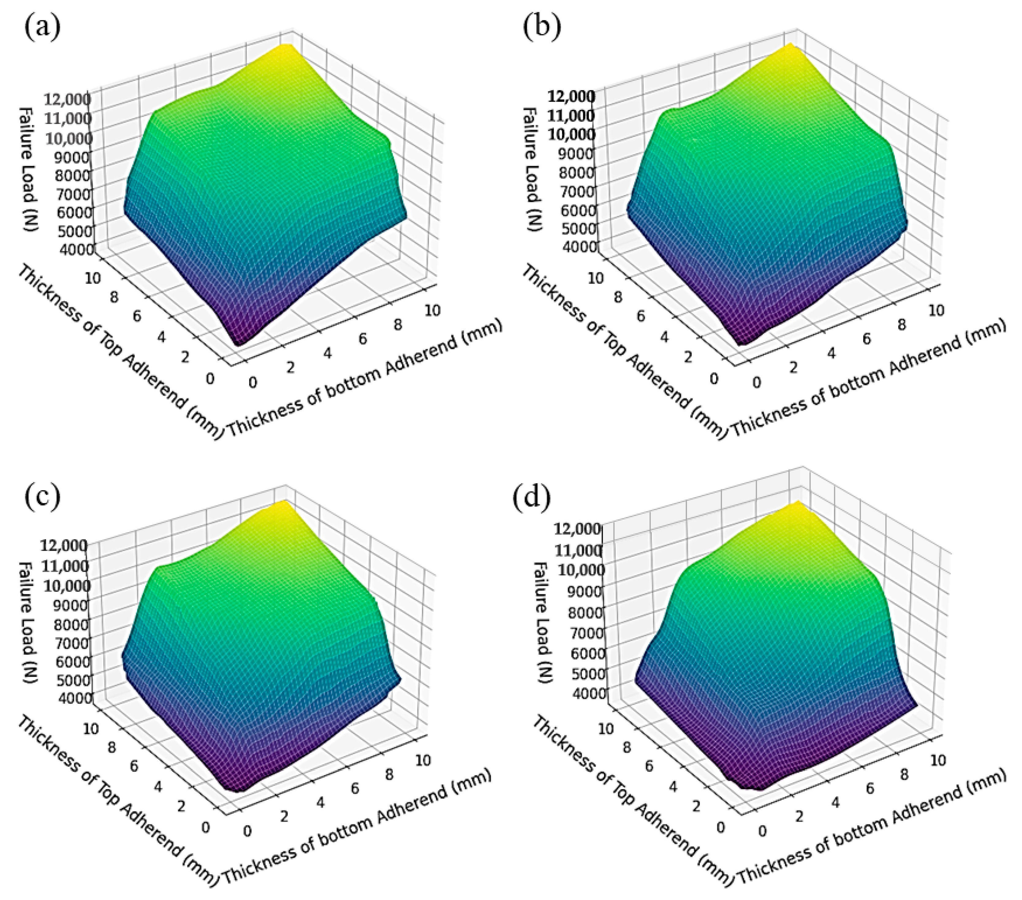
Figure 8 shows the response surfaces of joint failure load as a function of both upper and lower adherend thicknesses across four different adhesive thickness levels. In all cases, failure load exhibits a coupled and nonlinear dependence on the adherend thicknesses, with peak strength typically occurring when both top and bottom adherends fall within an intermediate-to-high thickness range. Figure 8a (t = 0.2 mm) shows a relatively steep and asymmetric failure load surface. This indicates that thinner adhesive layers make the joint more sensitive to variations in adherend thickness. Figure 8b,c show smoother surfaces with increased maximum strength. This suggests that thicker adhesive layers help buffer localized stress concentrations and enhance the synergy between adherends. However, Figure 8d shows an overall strength that plateaus or slightly declines, along with a flattened surface. This implies reduced sensitivity to further increases in adherend thickness. These trends reveal that the structural benefit of increasing adherend stiffness is most effectively realized when the adhesive thickness is within an optimal range—too thin leads to stress localization, while too thick may undermine load transfer efficiency. The consistent peak formation near the diagonal of each surface also suggests that balanced adherend design promotes more uniform stress distribution and higher joint integrity. Overall, these response surfaces highlight the intricate three-way interaction between top adherend, bottom adherend, and adhesive thickness, and confirm the DNN model’s ability to faithfully replicate such design-dependent mechanical behavior.

5.3. Analysis of Structural Optimization Results

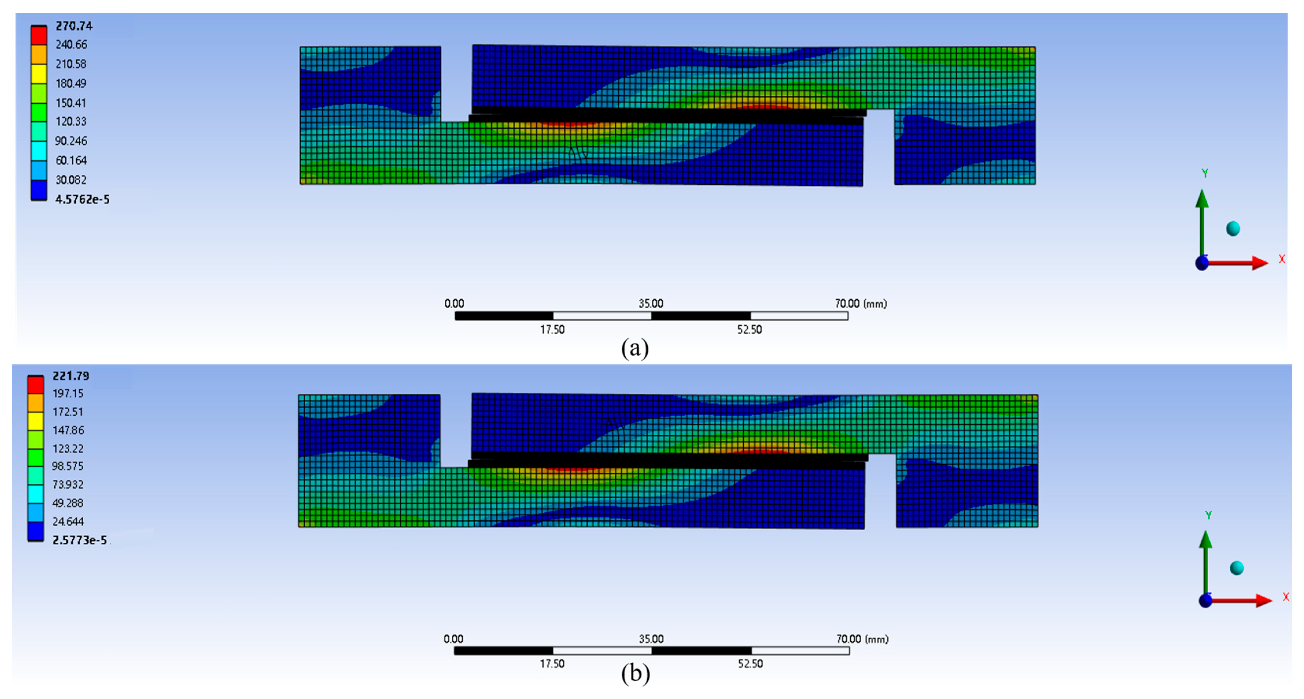
Table 4 shows the structural parameters obtained by the two optimization methods. The parameters of both are then input into the finite element model for calculation. Figure 9 presents the von Mises stress distributions of the optimized single-lap joints derived from the GA-DNN and response surface optimization (RSM) strategies, respectively. Both configurations exhibit typical stress concentrations near the ends of the adhesive layer—critical regions associated with damage initiation under tensile loading. However, clear differences emerge upon closer examination. The GA-optimized design (Figure 9a) demonstrates a more localized and higher-magnitude stress concentration along the interface, reflecting efficient load transfer and mechanical utilization of the adherend–adhesive system. In contrast, the RSM-optimized configuration (Figure 9b) displays a more diffuse stress field with lower peak values, suggesting a more conservative load-bearing mode and less optimized stress routing. The GA-DNN approach also leads to more efficient material usage, with slightly thinner components achieving better mechanical performance. Overall, the comparative stress fields reinforce the conclusion that the DNN-based surrogate model, when integrated with genetic algorithm optimization, not only yields more accurate predictions but also enables more structurally efficient and reliable joint designs.
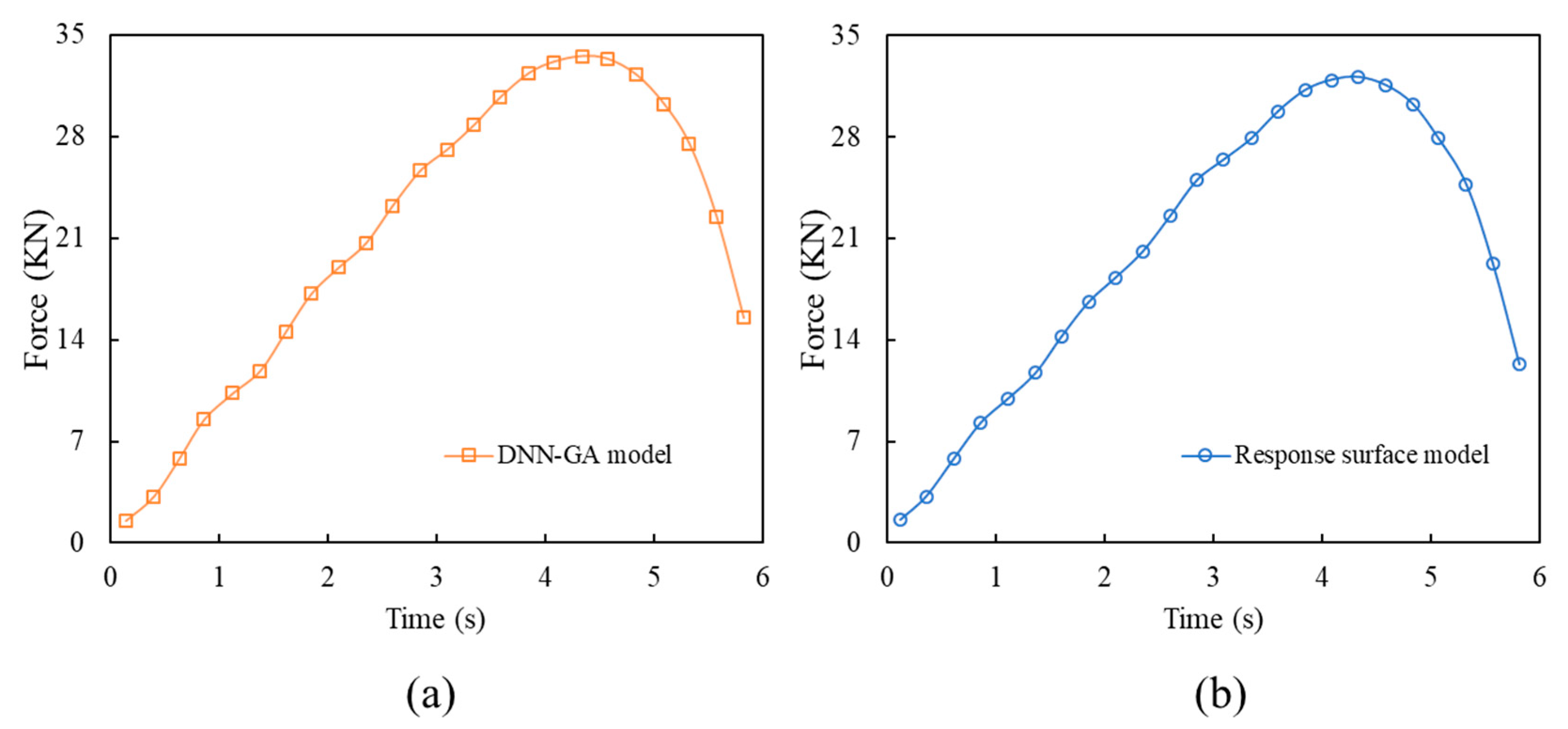
As shown in Figure 10 and Table 5, both curves experienced a break at around 4.25 s. Compared to the failure load F = 32,332 N obtained from the response surface optimization, the failure load value obtained by the GA optimization model was higher at F = 33,603 N. Moreover, the result of the GA optimization model had a smaller error compared to the prediction. The results demonstrate the practical advantage of the DNN-based surrogate in guiding high-performance adhesive joint design through robust optimization.
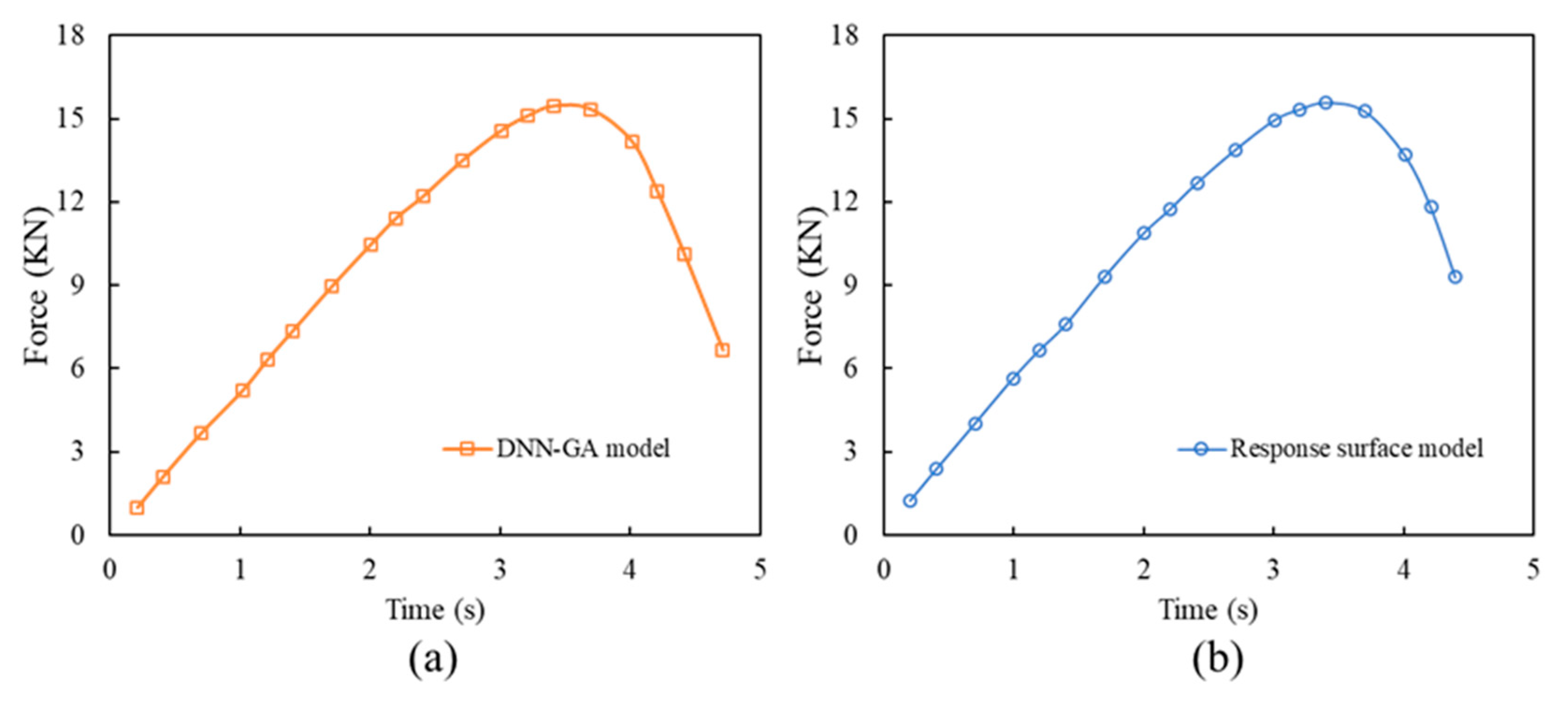
The structural parameters obtained through the GA model were t = 0.1014 mm, L = 29.9793 mm, T1 = 9.5386 mm, and T2 = 9.7597 mm. Figure 11 illustrates the von Mises stress distributions of two representative Pareto-optimal solutions obtained via multi-objective genetic algorithm (MOGA) optimization, aiming to balance joint strength and adhesive material usage. Both configurations demonstrate smooth stress transitions and well-distributed load transfer across the adhesive interface, validating the mechanical feasibility of the compromise designs. The failure loads obtained, respectively, were FGA = 15,651 N and FRSM = 15,498 N. By comparison, it can be seen that the structure obtained through multi-objective optimization based on GA is superior. In the case where the adhesive area was very close, the joint strength value increased by 153 N.
As shown in Figure 12, both curves exhibit the typical nonlinear behavior of adhesively bonded joints under tensile loading. The fracture occurred around 3.5 s. Due to the need to meet the requirements of multi-objective design, the optimized strength was lower than the result of single-objective optimization. The left-hand curve (orange) demonstrates a higher peak load, indicating a solution optimized for mechanical strength. Together, these results confirm that the MOGA-DNN optimization framework can effectively generate diverse high-performance designs along the Pareto front.

6. Conclusions

This study proposed an integrated framework that combines finite element modeling, deep learning, and evolutionary algorithms to predict and optimize the tensile strength of single-lap adhesive joints. A cohesive-zone-model-based finite element approach was first developed to simulate joint fracture behavior under varied geometric conditions. The simulation results not only captured the nonlinear damage evolution accurately but also provided a high-quality dataset for training data-driven models.
A deep neural network (DNN) was then constructed and trained using 300 data points generated via Latin Hypercube Sampling. The model demonstrated excellent predictive performance, with cross-validation R2 values consistently exceeding 0.98, indicating strong generalization capability. Serving as a surrogate model, the DNN was coupled with a genetic algorithm to carry out single-objective optimization aimed at maximizing joint strength. The optimized design yielded a validated tensile strength of 33,603 N, with a prediction error of just 1.49%, significantly outperforming response-surface-based optimization methods.
To further address real-world design constraints, a multi-objective genetic algorithm was applied to explore the trade-off between joint strength and adhesive volume. The resulting Pareto front revealed a set of compromise solutions, each reflecting different design priorities. Selected Pareto-optimal configurations were verified through finite element simulations, showing efficient stress transfer, favorable von Mises stress distributions, and mechanically sound load–displacement behavior.
These results collectively demonstrate that the DNN–GA/MOGA framework offers a robust, efficient, and accurate approach for the structural optimization of adhesively bonded joints. It enables rapid exploration of complex design spaces while maintaining high prediction fidelity, providing valuable guidance for engineering applications where strength, material efficiency, and structural reliability must be balanced. However, this method still has certain limitations. For example, it currently only considers continuous variables. Subsequent improvements could incorporate discrete variables (such as environmental factors and material properties). Future work may extend the method to fatigue life prediction, temperature-dependent performance optimization, and the design of multi-material or multi-joint adhesive systems. Furthermore, to meet different operational requirements, research on asymmetric joint designs could be conducted, further expanding its applicability in advanced structural engineering.

Author Contributions

Y.L.: Writing—Original Draft, Investigation, Methodology; Z.G.: Funding acquisition, Project administration, Writing—Review & Editing; M.S.: Visualization, Software; C.G.: Supervision, Validation; X.D.: Supervision, Formal analysis. All authors have read and agreed to the published version of the manuscript.

Funding

This research was funded by the Shandong Provincial Excellent Young Scientists Fund grant number 2024HWYQ-049, and the National Natural Science Foundation of China grant number: 12402109, and Qingdao Postdoctoral Science Foundation grant number QDBSH20240201002.

Data Availability Statement

The raw data supporting the conclusions of this article will be made available by the authors on request.

Conflicts of Interest

The authors declare no conflict of interest.

References

  1. Beevers, A.; Steidler, S.M.; Durodola, J.; Coackley, M. Analysis of stiffness of adhesive joints in car bodies. J. Mater. Process. Technol. 2001, 118, 95–100. [Google Scholar] [CrossRef]
  2. Scarselli, G.; Corcione, C.; Nicassio, F.; Maffezzoli, A. Adhesive joints with improved mechanical properties for aerospace applications. Int. J. Adhes. Adhes. 2017, 75, 174–180. [Google Scholar] [CrossRef]
  3. Goland, M.; Reissner, E. The Stresses in Cemented Joints. J. Appl. Mech. 1944, 11, A17–A27. [Google Scholar] [CrossRef]
  4. Hart-Smith, L.J. Adhesive-Bonded Single-Lap Joints; Report NASA [74]CR-112236; NASA Langley Research Center: Hampton, VA, USA, 1973.
  5. Zhao, B.; Lu, Z.-H.; Lu, Y.-N. Closed-form solutions for elastic stress–strain analysis in unbalanced adhesive single-lap joints considering adherend deformations and bond thickness. Int. J. Adhes. Adhes. 2011, 31, 434–445. [Google Scholar] [CrossRef]
  6. Zhao, B.; Lu, Z.-H.; Lu, Y.-N. Two-dimensional analytical solution of elastic stresses for balanced single-lap joints—Variational method. Int. J. Adhes. Adhes. 2014, 49, 115–126. [Google Scholar] [CrossRef]
  7. Chen, D.; Cheng, S. An Analysis of Adhesive-Bonded Single-Lap Joints. J. Appl. Mech. 1983, 50, 109–115. [Google Scholar] [CrossRef]
  8. Cheng, S.; Chen, D.; Shi, Y. Analysis of Adhesive-Bonded Joints with Nonidentical Adherends. J. Eng. Mech. 1991, 117, 605–623. [Google Scholar] [CrossRef]
  9. Arenas, J.M.; Narbón, J.J.; Alía, C. Optimum adhesive thickness in structural adhesives joints using statistical techniques based on Weibull distribution. Int. J. Adhes. Adhes. 2010, 30, 160–165. [Google Scholar] [CrossRef]
  10. Öz, Ö.; Özer, H. An experimental investigation on the failure loads of the mono and bi-adhesive joints. J. Adhes. Sci. Technol. 2017, 31, 2251–2270. [Google Scholar] [CrossRef]
  11. Bendemra, H.; Compston, P.; Crothers, P.J. Optimisation study of tapered scarf and stepped-lap joints in composite repair patches. Compos. Struct. 2015, 130, 1–8. [Google Scholar] [CrossRef]
  12. Sülü, İ.Y. Mechanical behavior of composite parts adhesively jointed with the insert double-lap joint under tensile load. Weld. World 2018, 62, 403–413. [Google Scholar] [CrossRef]
  13. Gong, B.; Li, H. A couple Voronoi-RBSM modeling strategy for RC structures. Struct. Eng. Mech. 2024, 91, 239–250. [Google Scholar]
  14. Xu, H.; Cui, X.; Liu, Y.; Xu, Y.; Ling, X.; Li, Y. Effect of Fastening System Failure on the Micromechanical Properties of Railway Ballast Bed. KSCE J. Civ. Eng. 2025, 29, 100233. [Google Scholar] [CrossRef]
  15. Cao, L.; Lu, R.; Dou, Z.; Zheng, M.; Han, X.; Hao, Y.; Zhang, L.; Zhang, J.; Liu, B.; Li, X. Understanding the influence of high-strength submicron precipitate on the fracture performance of additively-manufactured aluminum alloy. Int. J. Plast. 2025, 188, 104306. [Google Scholar] [CrossRef]
  16. Gao, J.; Wang, S.; Zhang, C.; Chen, R.; Zhang, Y.; Zhang, Y.; Mu, R. Energy-based multi-axial fatigue prediction for tubular structures under non-proportional loading. Int. J. Fatigue 2025, 197, 108897. [Google Scholar] [CrossRef]
  17. Gu, Z.; Liu, Y.; Hughes, D.J.; Ye, J.; Hou, X. A parametric study of adhesive bonded joints with composite material using black-box and grey-box machine learning methods: Deep neuron networks and genetic programming. Compos. Part B Eng. 2021, 217, 108894. [Google Scholar] [CrossRef]
  18. Wang, C.; Zhang, Z.; Jing, X.; Yang, Z.; Xu, W. Optimization of multistage femtosecond laser drilling process using machine learning coupled with molecular dynamics. Opt. Laser Technol. 2022, 156, 108442. [Google Scholar] [CrossRef]
  19. Zhang, Z.; Liu, S.; Zhang, Y.; Wang, C.; Zhang, S.; Yang, Z.; Xu, W. Optimization of low-power femtosecond laser trepan drilling by machine learning and a high-throughput multi-objective genetic algorithm. Opt. Laser Technol. 2022, 148, 107688. [Google Scholar] [CrossRef]
  20. Mashrei, M.A.; Seracino, R.; Rahman, M.S. Application of artificial neural networks to predict the bond strength of FRP-to-concrete joints. Constr. Build. Mater. 2013, 40, 812–821. [Google Scholar] [CrossRef]
  21. Rangaswamy, H.; Sogalad, I.; Basavarajappa, S.; Acharya, S.; Patel, G.C.M. Experimental analysis and prediction of strength of adhesive-bonded single-lap composite joints: Taguchi and artificial neural network approaches. SN Appl. Sci. 2020, 2, 1055. [Google Scholar] [CrossRef]
  22. Wang, Z.; Li, J.; Yuan, Y.; Zhang, S.; Hu, W.; Ma, J.; Tan, J. Digital-twin-enabled online wrinkling monitoring of metal tube bending manufacturing: A multi-fidelity approach using forward-convolution-GAN. Appl. Soft Comput. 2025, 171, 112684. [Google Scholar] [CrossRef]
  23. Cevik, A.; Arslan, M.H.; Köroğlu, M.A. Genetic-programming-based modeling of RC beam torsional strength. KSCE J. Civ. Eng. 2010, 14, 371–384. [Google Scholar] [CrossRef]
  24. Pala, M. Genetic programming-based formulation for distortional buckling stress of cold-formed steel members. J. Constr. Steel Res. 2008, 64, 1495–1504. [Google Scholar] [CrossRef]
  25. Ravandi, E.G.; Rahmannejad, R.; Monfared, A.E.F.; Ravandi, E.G. Application of numerical modeling and genetic programming to estimate rock mass modulus of deformation. Int. J. Min. Sci. Technol. 2013, 23, 733–737. [Google Scholar] [CrossRef]
  26. Feng, X.; Zhao, J.; Kita, E. Genetic Algorithm-based Optimization of Deep Neural Network Ensemble. Rev. Socionetwork Strateg. 2021, 15, 27–47. [Google Scholar] [CrossRef]
  27. Al-Mosawe, A.; Kalfat, R.; Al-Mahaidi, R. Strength of Cfrp-steel double strap joints under impact loads using genetic programming. Compos. Struct. 2017, 160, 1205–1211. [Google Scholar] [CrossRef]
  28. Elices, M.; Guinea, G.V.; Gómez, J.; Planas, J. The cohesive zone model: Advantages, limitations and challenges. Eng. Fract. Mech. 2002, 69, 137–163. [Google Scholar] [CrossRef]
  29. Needleman, A. An analysis of decohesion along an imperfect interface. Int. J. Fract. 1990, 42, 21–40. [Google Scholar] [CrossRef]
  30. Reedy, E.D.; Guess, T.R. Comparison of butt tensile strength data with interface corner stress intensity factor prediction. Int. J. Solids Struct. 1993, 30, 2929–2936. [Google Scholar] [CrossRef]
  31. Irwin, G.R.; Paris, P.C. Chapter 1—Fundamental Aspects of Crack Growth and Fracture. In Engineering Fundamentals and Environmental Effects; Liebowitz, H., Ed.; Academic Press: Cambridge, MA, USA, 1971; pp. 1–46. [Google Scholar]
  32. Kanani, A.Y.; Wang, X.-E.; Hou, X.; Rennie, A.E.W.; Ye, J. Analysis of failure mechanisms of adhesive joints modified by a novel additive manufacturing-assisted method. Eng. Struct. 2023, 277, 115428. [Google Scholar] [CrossRef]
  33. Olsson Anders, M.J.; Sandberg Göran, E. Latin Hypercube Sampling for Stochastic Finite Element Analysis. J. Eng. Mech. 2002, 128, 121–125. [Google Scholar] [CrossRef]
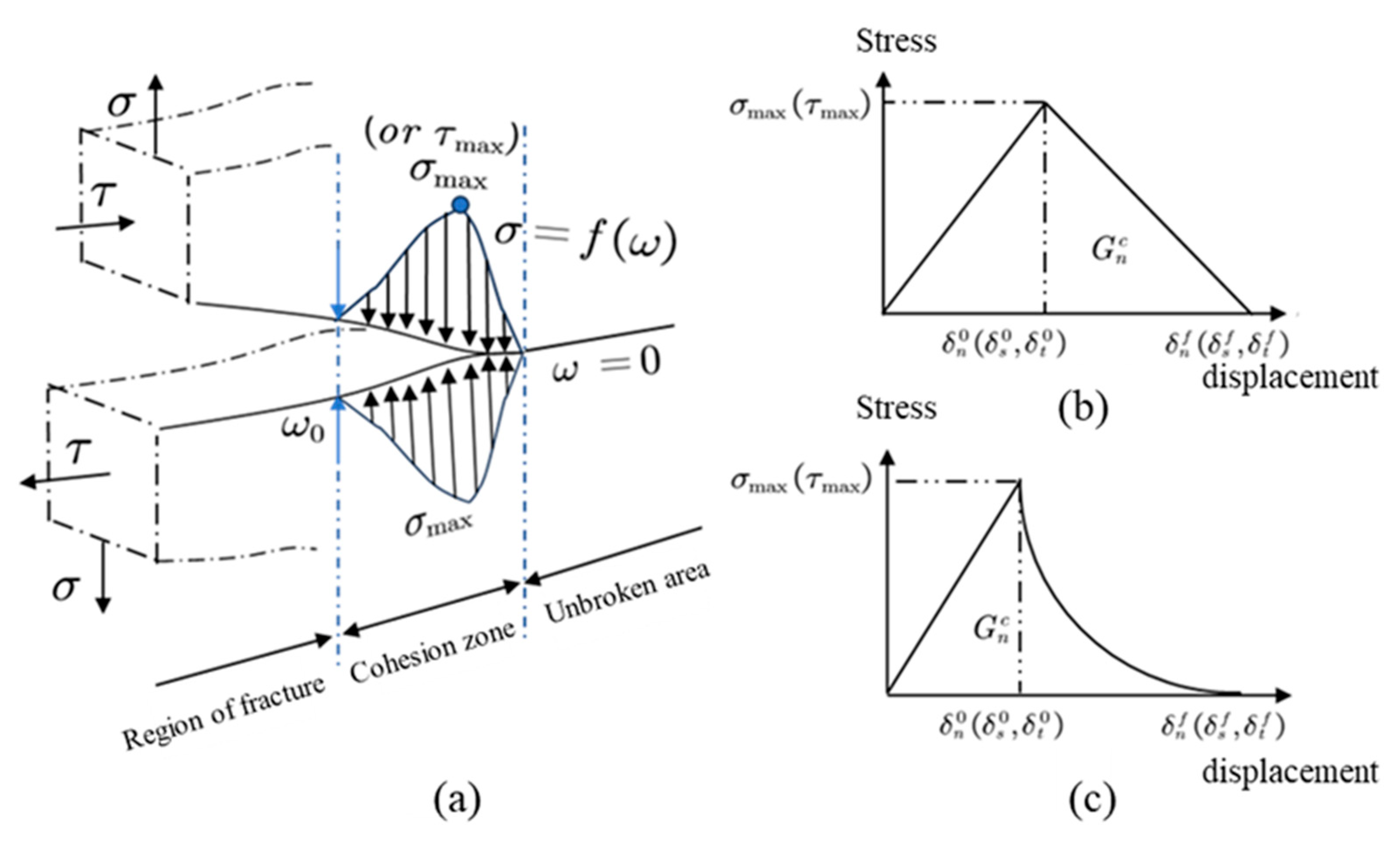
Figure 1. (a) Schematic diagram of the cohesion model. (b) Double-linear damage rule. (c) Exponential damage rule.
Applsci 15 09041 g001
Figure 2. Boundary conditions and mesh settings of the finite element model.
Applsci 15 09041 g002
Figure 3. Overall schematic diagram of the deep neural network used for predicting the strength of a single-lap joint.
Applsci 15 09041 g003
Figure 4. Force–displacement curves for adhesive joint.
Applsci 15 09041 g004
Figure 5. Verification diagrams of deep neural network joint strength training results for different training groups and test groups: (a) Test Group 1, (b) Test Group 2, (c) Test Group 3, (d) Training Group 1, (e) Training Group 2, (f) Training Group 3.
Applsci 15 09041 g005
Figure 6. Response surface results of adhesive layer thickness and lap length under different upper adhesive body thicknesses T1: (a) T2 = 1 mm, (b) T2 = 4 mm, (c) T2 = 7 mm, (d) T2 = 10 mm.
Applsci 15 09041 g006
Figure 7. Response surface results of the thickness of the upper adhesive body and the lap length with different adhesive layer thicknesses t: (a) t = 0.2 mm, (b) t = 0.8 mm, (c) t = 1.4 mm, (d) t = 2 mm.
Applsci 15 09041 g007
Figure 8. Response surfaces of the upper adherent thickness and the lower adherent thickness at different adhesive layer thicknesses t: (a) t = 0.2 mm, (b) t = 0.8 mm, (c) t = 1.35 mm, (d) t = 2 mm.
Applsci 15 09041 g008
Figure 9. The stress results obtained after optimizing the parameters of a single objective and incorporating them into the finite element model. (a): GA optimization, (b): Response surface optimization.
Applsci 15 09041 g009
Figure 10. Curve of download load variation over time for the two single-objective optimization methods. (a): GA optimization, (b): Response surface optimization.
Applsci 15 09041 g010
Figure 11. The stress results obtained after optimizing the parameters of a multi objective and incorporating them into the finite element model. (a): GA optimization, (b): Response surface optimization.
Applsci 15 09041 g011
Figure 12. Curve of download load variation over time for the two multiple-objective optimization methods. (a): GA optimization, (b): Response surface optimization.
Applsci 15 09041 g012
Table 1. The range of values for parameterized variables.
Parametric VariablesLower LimitUpper Limit
Bonding length, La (mm)1070
Thickness of the top adherent, T1 (mm)110
Thickness of the bottom adherent, T2 (mm)110
Adhesive thickness, t (mm)0.14
Table 2. Basic properties of materials.
MaterialsYoung Modulus (GPa)Poisson’s Ratio
Al 6082T670.000.30
Araldite 20151.850.33
Table 3. Fracture properties of adhesives.
Adhesive NameTensile Breaking StrengthShear Failure StrengthTensile ToughnessShear Toughness
Araldite 201521.63 (MPa)17.90 (MPa)0.43 (J/mm2)4.7 (J/mm2)
Table 4. The optimized parameters of the two models.
ModelGA OptimizationResponse Surface Optimization
Adhesive thickness (mm)1.125051.25978
Bonding length (mm)69.968570
Thickness of the top adherent (mm)9.8570210
Thickness of the bottom adherent (mm)9.8871710
Adhesive thickness (mm)1.125051.25978
Table 5. Comparison of the results of the two optimization models.
ModelGA OptimizationResponse Surface Optimization
Predicted value (N) 33,10333,564
Verification value (N) 33,60332,332
Error1.49%3.81%
Disclaimer/Publisher’s Note: The statements, opinions and data contained in all publications are solely those of the individual author(s) and contributor(s) and not of MDPI and/or the editor(s). MDPI and/or the editor(s) disclaim responsibility for any injury to people or property resulting from any ideas, methods, instructions or products referred to in the content.