Synthetic Aperture Radar (SAR) Data Compression Based on Cosine Similarity of Point Clouds

Abstract

This paper proposes a structure-aware compression technique for efficient compression of high-resolution synthetic aperture radar (SAR)-based point clouds by quantitatively analyzing the directional characteristics of local structures. The proposed method computes the angular difference between the principal eigenvector of each point and those of its neighboring points, selectively removing points with low contribution to directional preservation and retaining only structurally significant feature points. The method demonstrates superior information preservation performance through various compression evaluation metrics such as entropy, peak signal-to-noise ratio (PSNR), and structural similarity index measure (SSIM). Additionally, the SHREC’19 human mesh dataset is employed to further assess the generality and robustness of the proposed approach. The results show that the proposed method can maximize data efficiency while preserving the core information of the point cloud through a novel directionality-based structural preservation strategy.

1. Introduction

A point cloud [1,2] is a data structure that represents objects or environments in 3D space as a collection of discrete points. It has become a critical component in various spatial perception-based applications such as autonomous driving [3,4], robotic vision [5], augmented and virtual reality (AR/VR), smart city planning, and restoration of cultural heritage. Traditionally, point clouds are acquired through various 3D sensors, including RGB-D sensors, multiview stereo cameras, LiDAR, and RADAR, and they provide high-precision data containing 3D coordinates (x, y, z), as well as attribute information such as color (R, G, B), reflectance intensity, velocity, and more.

Conventional fixed-position radar systems [6,7] operate by emitting pulses from a stationary transmitter and receiving reflected signals at a single observation point. In contrast, synthetic aperture radar (SAR) [8,9] collects reflected signals from multiple positions as the sensor moves continuously over time, accumulating and synthesizing them. By combining multiple reflections acquired from different observation points, SAR effectively simulates the functionality of a large physical antenna. This enables it to generate high-density 3D data with much more observational information than standard fixed radar systems. Unlike traditional radar, SAR systems incorporate both temporal accumulation and spatial diversity, allowing for highly detailed representation of complex high-dimensional structures. However, this advantage also comes with a significant trade-off. The data increase rapidly due to the high point density and complex structural information. For example, an SAR system with 12 transmit antennas (Tx) and 16 receive antennas (Rx), forming a 192-channel setup, may generate a scan with 32 chirps and 1024 samples per chirp. At a rate of 20 scans per second, this results in 125,829,120 complex samples per second (192 channel × 32 Chirp × 1024 sample × 20 scan). Since each complex sample consists of a real and imaginary part, each represented by 16 bits (2 bytes), the system produces approximately 4.03 Gbps (4,026,531,840 bits/s ) of raw data per second. Although SAR-based high-density point clouds provide excellent spatial and visual expressiveness, their massive size makes real-time analysis or cloud-based computation virtually impossible without compression techniques. Therefore, efficient compression methods are essential to preserve critical information while minimizing data loss.

In LiDAR, the commonly used compression method is geometry-based point cloud compression (G-PCC), which is a structure-based algorithm that improves compression efficiency by spatially dividing the point cloud into octree [10,11,12,13] or voxel structures and removing redundant information. G-PCC is well suited for LiDAR data that have a precise and uniformly distributed point density. Representative research based on G-PCC includes HPSR-PCGC [14], which applies hierarchical super-resolution reconstruction to enable fine structural restoration, VPO [15], which improves LiDAR sequence compression efficiency through vertical object-based motion prediction, MS-GAT [16], which transforms point clouds into graph structures and learns multiscale correlations, and an SMPL template-based compression method [17], optimized for human shape reconstruction. In this study, rather than following traditional octree- or voxel-based target structure compression methods, we focus on the directionality inherent in point clouds. Unlike LiDAR, SAR-based point clouds are reconstructed by accumulating reflected signals from various observation points, and thus, even within the same object, different point clouds can be affected differently in terms of their structural directionality. This characteristic of the data structure raises the need for a precise compression strategy that reflects the contribution of each point cloud to structural directionality.

In this study, we propose a selective compression method that quantitatively analyzes the directionality inherent in SAR-based point clouds, preserving structurally important directional information and removing less important point clouds. The proposed method constructs a covariance matrix between each point and its neighboring points and decomposes it into eigenvectors through principal component analysis (PCA), thereby extracting the main directionality of the corresponding region. Then, by comparing the directional difference ($\theta$) between the principal eigenvectors of the local point cloud that include the reference point and exclude the reference point, the method quantitatively evaluates the extent to which the reference point contributes to maintaining the directional structure of the region. If the $\theta$ value is small, it indicates that the structural directionality of the region is maintained regardless of whether the reference point is included; so, the point is considered nonimportant and can be removed. On the other hand, if the $\theta$ value is large, the reference point is regarded as a structural key point that determines the directional structure of the region and must be preserved. By applying this directionality-based evaluation criterion to compress the point cloud, the proposed method can minimize information loss and maximize compression efficiency while considering the spatial directionality of SAR point clouds.

2. Materials and Methods

2.1. FMCW-Based SAR System and Point Cloud Generation

Based on the raw data received from the FMCW radar, distance and angle information were extracted and converted into 3D coordinates to generate the point cloud. The specifications of the FMCW radar used (AFI910, BitSensing, Seongnam-si, South Korea ) are shown in

Table 1. Radar parameters (AFI910, BitSensing).

Parameter	Value
Center Frequency ($F_c$)	79 GHz
Chirp Duration ($T_c$)	256 µs
Sampling Frequency ($F_s$)	4 MHz
Number of Channels ($N_{\mathrm{ch}}$)	192 (12 Tx × 16 Rx)
Number of Chirps ($N_{\mathrm{chirp}}$)	32
Number of Samples ($N_{\mathrm{samples}}$)	1024
Chirp Interval	0.05 Section (20 fps)
Bandwidth (SR/MR)	3.0 GHz/2.2 GHz
Range Resolution (SR)	0.05 m (≈5 cm)
Range Resolution (MR)	0.068 m (≈6.8 cm)
Azimuth Field of View (FOV)	±45°
Elevation Field of View (FOV)	±15°

.

A radar sensor was mounted on a linear stage, as shown in Figure 1. The linear stage was installed at a height of 0.1 meters above the ground, facing directly toward the target. The sensor’s radiation direction was tilted 15° upward.

Table 2. Linear stage parameters according to scanning speed conditions.

Condition	5 mm/s	10 mm/s	15 mm/s	20 mm/s
Scan Time (s)	160	80	55	40
Scan Count	1600	800	550	400

presents the scan time and number of scans corresponding to different scan speeds of the linear stage.

The FMCW radar transmits a frequency-modulated continuous wave whose frequency changes linearly over time and receives signals reflected from the target [18,19]. It analyzes the beat signal between the transmitted and received waveforms. For each antenna channel, a one-dimensional FFT (1D FFT) along the sample axis of the chirp signal generates a range spectrum from which the target distance is extracted. Based on this range spectrum, phase variations across multiple chirps within the same range bin are analyzed; a two-dimensional FFT (2D FFT) along the chirp dimension extracts the Doppler component, resulting in a Doppler (velocity) spectrum. For the resulting range–velocity map, noncoherent integration (NCI) across all channels accumulates magnitudes to improve the signal-to-noise ratio (SNR). A 2D constant false alarm rate (CFAR) detector is then applied to automatically detect peaks in the range–velocity map. The 2D FFT values at the detected peak positions are stored for subsequent angle estimation. For each target detected by CFAR, the Bartlett beamforming method is applied to estimate the angle. Finally, using the estimated range and angles, a 3D point cloud is generated. In this study, we reconstruct a 3D representation of the observed scene from the SAR signals by transforming the estimated range and angle parameters into Cartesian coordinates. Specifically, for each detected target, the range r, azimuth angle $\varphi$, and elevation angle $\theta$ are obtained from the radar signal-processing chain described above. These parameters represent the location of the reflector in a spherical coordinate system centered at the radar sensor. To convert these into 3D Cartesian coordinates $(x,y,z)$, we apply the following transformation:

$$x=rcos\theta sin\varphi$$

(1)

$$y=rcos\theta cos\varphi$$

(2)

$$z=rsin\theta$$

(3)

Here, the azimuth angle $\varphi$ is measured in the horizontal plane relative to the radar’s boresight, and the elevation angle $\theta$ is measured in the vertical plane. These angles are obtained via the Bartlett beamforming algorithm applied over the MIMO antenna array, while the range r is determined from the 1D FFT of the chirp signal. The signal-processing flowchart for radar-based point cloud generation is illustrated in Figure 2.

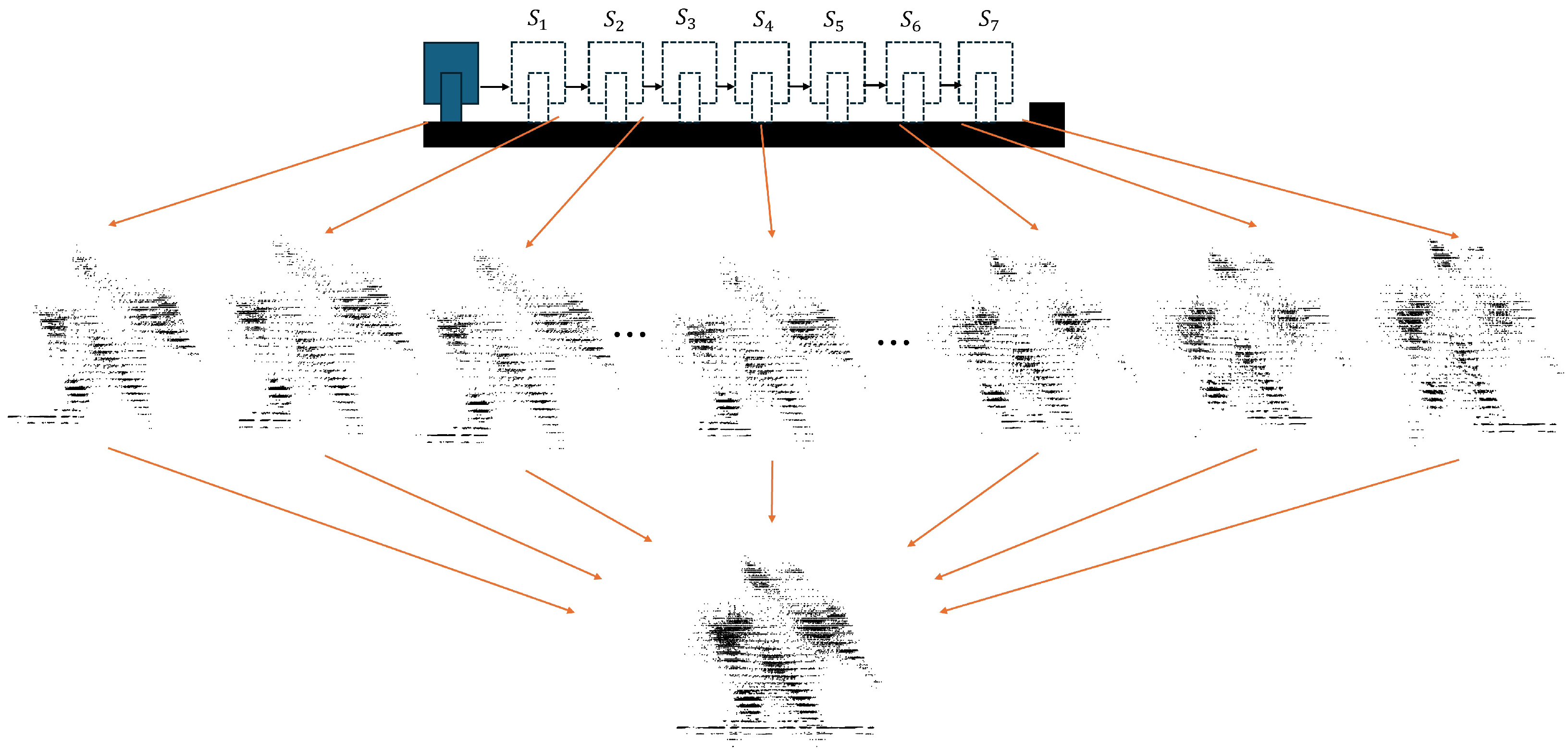
Each scan acquired by the radar sensor as it moves along the linear stage is taken at fixed time intervals and at a constant speed. However, since each scan is captured from a different physical location, directly merging the scans may cause spatial distortion. To correct this issue, the Y-coordinate of each scan is adjusted by accounting for the radar’s movement distance. Let the k-th scan be denoted as $S_k$, and let the coordinates of the point cloud from $S_k$ be $(x_k,y_k,z_k)$. The accumulated movement distance of the radar is given by

$$d_k=v·\Delta t,$$

(4)

where v is the scan velocity and $\Delta t$ is the time interval between scans. The corrected Y-coordinate ${\widehat{y}}_k$ is then calculated as

$${\widehat{y}}_k=y_k+d_k.$$

(5)

As a result, the corrected point cloud coordinates of the k-th scan become $(x_k,{\widehat{y}}_k,z_k)$. By combining each scan in this manner along the Y-axis, the final data are constructed as a three-dimensional point cloud. The 3D point cloud generated by the radar includes not only the target shape but also background elements, surrounding structures, and noise. Therefore, a preprocessing step is required to remove unnecessary points before compression is applied. In this study, we applied the Density-Based Spatial Clustering of Applications with Noise (DBSCAN) algorithm to automatically extract the primary cluster corresponding to the target shape, as shown in Figure 3.

2.2. Novel Point Cloud Compression Based on Cosine Similarity

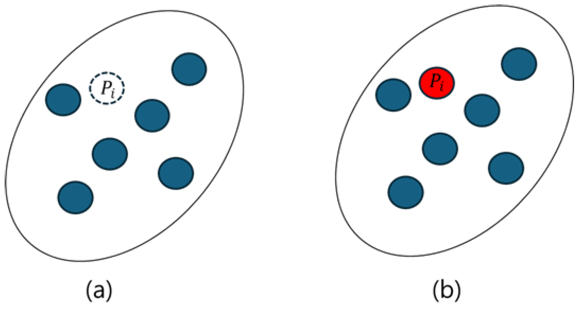
In this study, we propose a directionality-based key point preservation strategy for the efficient compression of point cloud data. This approach selectively retains only structurally meaningful points by analyzing the directional similarity of eigenvectors between each point and its neighboring points. Let the point cloud be defined as $P=\{p_1,p_2,\dots ,p_M\}$, where M is the total number of points. For each reference point $p_i$, where $i\in \{1,2,\dots ,M\}$, we calculate the Euclidean distances to all other points in order to identify its K nearest neighbors. Let ${\mathcal{I}}_i\subset \{1,2,\dots ,M\}\setminus \left\{i\right\}$ be the index set of the K nearest neighbors of point $p_i$, satisfying the condition $|{\mathcal{I}}_i|=K$. Then, the neighbor point set is defined as

$${\mathcal{N}}_i=\{p_j\mid j\in {\mathcal{I}}_i\}.$$

(6)

Furthermore, we define the augmented set that includes the reference point and its neighbors as

$${\mathcal{N}}_i^p={\mathcal{N}}_i\cup \left\{p_i\right\}.$$

(7)

The two point sets are illustrated in Figure 4.

To quantify the directional characteristics of the local structural distribution, a covariance matrix is computed for each point set. For the point set ${\mathcal{N}}_i^p$, which includes the reference point $p_i$ and its N nearest neighbors ${\mathcal{N}}_i$ ($i=1,2,3,\dots ,N$), and for the point set ${\mathcal{N}}_i$, which excludes the reference point, the covariance matrices ${\Sigma }_i^p$ and ${\Sigma }_i$ are defined as follows:

$${\Sigma }_i^p=\mathrm{cov}\left({\mathcal{N}}_i^p\right),$$

(8)

$${\Sigma }_i=\mathrm{cov}\left({\mathcal{N}}_i\right).$$

(9)

Given a point set $\mathcal{S}=\{p_1,p_2,\dots ,p_n\}\subset {\mathbb{R}}^3$, the covariance matrix $\mathrm{cov}\left(\mathcal{S}\right)$ is defined as

$$\mathrm{cov}\left(\mathcal{S}\right)={\displaystyle \frac{1}{n}}\sum _{k=1}^n\left(p_k-\overline{p}\right){\left(p_k-\overline{p}\right)}^{\top },$$

(10)

where $\overline{p}={\displaystyle \frac{1}{n}}{\sum }_{k=1}^n{p}_k$ is the centroid of $\mathcal{S}$. These covariance matrices quantify how widely the point sets are distributed in different directions. The previously computed covariance matrices ${\Sigma }_i^p$ and ${\Sigma }_i$ encode the local spatial distribution, from which dominant directional features can be extracted. To this end, we perform eigenvalue decomposition. The eigenvalues ${\lambda }_k^p,{\lambda }_k$ and the corresponding eigenvectors ${\mathbf{v}}_k^p,{\mathbf{v}}_k$ of ${\Sigma }_i^p$ and ${\Sigma }_i$ are defined as

$${\Sigma }_i^p{\mathbf{v}}_k^p={\lambda }_k^p{\mathbf{v}}_k^p,k=1,2,3,$$

(11)

$${\Sigma }_i{\mathbf{v}}_k={\lambda }_k{\mathbf{v}}_k,k=1,2,3.$$

(12)

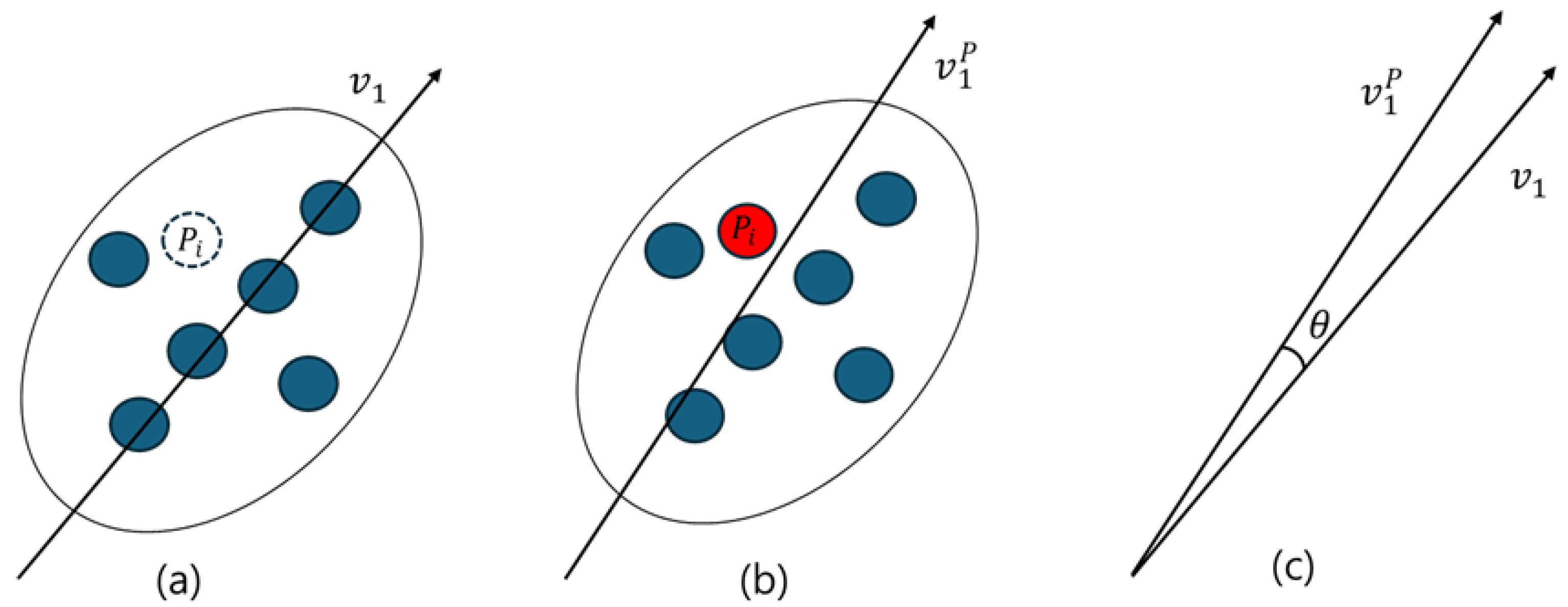
Among them, the eigenvectors ${\mathbf{v}}_1^p$ and ${\mathbf{v}}_1$ associated with the largest eigenvalue (assuming ${\lambda }_1>{\lambda }_2>{\lambda }_3$) are taken as the principal directions of the respective sets. To quantify the influence of the reference point on the local structure, we compare the angular difference between ${\mathbf{v}}_1^p$ and ${\mathbf{v}}_1$, computed on ${\mathcal{N}}_i^p$ (including $p_i$) and ${\mathcal{N}}_i$ (excluding $p_i$), respectively. The angle $\theta$ is given by

$$\theta ={cos}^{-1}\left({\displaystyle \frac{{\mathbf{v}}_1^p·{\mathbf{v}}_1}{\parallel {\mathbf{v}}_1^p\parallel \parallel {\mathbf{v}}_1\parallel }}\right).$$

(13)

The principal eigenvectors and their angular difference are illustrated in Figure 5.

The closer the angular difference $\theta$ between the two principal eigenvectors is to $0°$, the more similar the principal directions of the point sets with and without the reference point are. This indicates that the reference point has little influence on the local structure. Conversely, a larger value of $\theta$ implies that the principal direction changes significantly depending on the presence of the reference point, suggesting that the point plays an important role in forming the local structure. Accordingly, if the angle ${\theta }_i$ exceeds a certain threshold ${\theta }_{\mathrm{th}}$, the reference point $p_i$ is identified as a structural key point and is preserved. Otherwise, the point is considered removable to achieve compression while minimizing the loss of information:

$$\mathrm{Decision}\mathrm{on}{p}_i=\left\{\begin{array}{cc}\mathrm{conserve}{p}_i,\hfill & \mathrm{if}{\theta }_i\ge {\theta }_{\mathrm{th}}\hfill \\ \mathrm{remove}{p}_i,\hfill & \mathrm{if}{\theta }_i<{\theta }_{\mathrm{th}}\hfill \end{array}\right..$$

(14)

By directly comparing the directional changes of local structures within the point cloud using this method, a more precise and selective preservation of important points can be achieved, enabling a directionality-based compression strategy. The compression rate can be controlled using the threshold ${\theta }_{\mathrm{th}}$, where a larger ${\theta }_{\mathrm{th}}$ results in a higher compression rate.

3. Discussion

In this experiment, the subject stood stationary at a distance of $3.0\mathrm{m}$ from the radar sensor, with a height of $1.82\mathrm{m}$. The radar sensor moved along the linear stage over a total distance of $0.8\mathrm{m}$ at a speed of $5\mathrm{mm}/\mathrm{s}$. The scan interval was fixed at $100\mathrm{ms}$, resulting in the collection of 1600 frames of point-cloud data over $160\mathrm{s}$. As shown in Figure 6, the sensor was tilted upward by $15°$ relative to the horizontal plane to observe the human body. The sensor’s lateral movement allowed it to capture reflected signals from multiple perspectives, enabling multi-angle acquisition of the static human shape.

To quantitatively evaluate the structure-preserving performance of the proposed point cloud compression method, the SHREC’19 Track: Matching Humans with Different Connectivity dataset was additionally utilized. This dataset consists of hundreds of 3D human mesh pairs with varying mesh connectivity and vertex density, providing data suitable for assessing the robustness of algorithms in realistic shape matching scenarios. The correspondence between each mesh pair is computed using the functional automatic registration method (FARM) [20], which is based on the skinned multi-person linear (SMPL) [21] statistical human model, ensuring high-quality ground-truth data. This allows for a precise comparison and evaluation of structural preservation in the point clouds before and after compression.

Table 3. Summary of point cloud compression performance based on local structure (using $\theta$ thresholds).

Item	SAR-Based Data	SHREC’19 Mesh Data
Total Number of Points ($N_{\mathrm{original}}$)	32,964 points	27,061 points
Number of Removed Points	16,295 points (49.44%)	13,774 points (50.89%)
Preserved Key Points ($N_{\mathrm{remaining}}$)	16,669 points (50.56%)	13,287 points (49.11%)
Average Structural Angle ($\theta$)	$2.3375°$	$0.6586°$
Selected Threshold (${\theta }_{\mathrm{th}}$)	$0.6°$	$0.25°$
Compression Ratio (CR)	Approx. 2.0:1	Approx. 2.0:1

presents an example case where the compression ratio is maintained at approximately 2.0:1. For the SAR data, compression was performed using a threshold of $\theta =0.6°$, resulting in an average structural angle of approximately $2.3375°$. Out of a total of 32,964 points, only 16,669 structural key points were selectively preserved, achieving a compression ratio of about 2.0:1. In contrast, for the SHREC’19 mesh data, using a threshold of $\theta =0.25°$, the average structural angle was measured as $0.6586°$. From a total of 27,061 points, 13,287 structural key points were preserved, also achieving a compression ratio of approximately 2.0:1. The compression ratio is defined as

$$\mathrm{Compression}\mathrm{Ratio}\left(\mathrm{CR}\right)={\displaystyle \frac{N_{\mathrm{original}}}{N_{\mathrm{remaining}}}}.$$

(15)

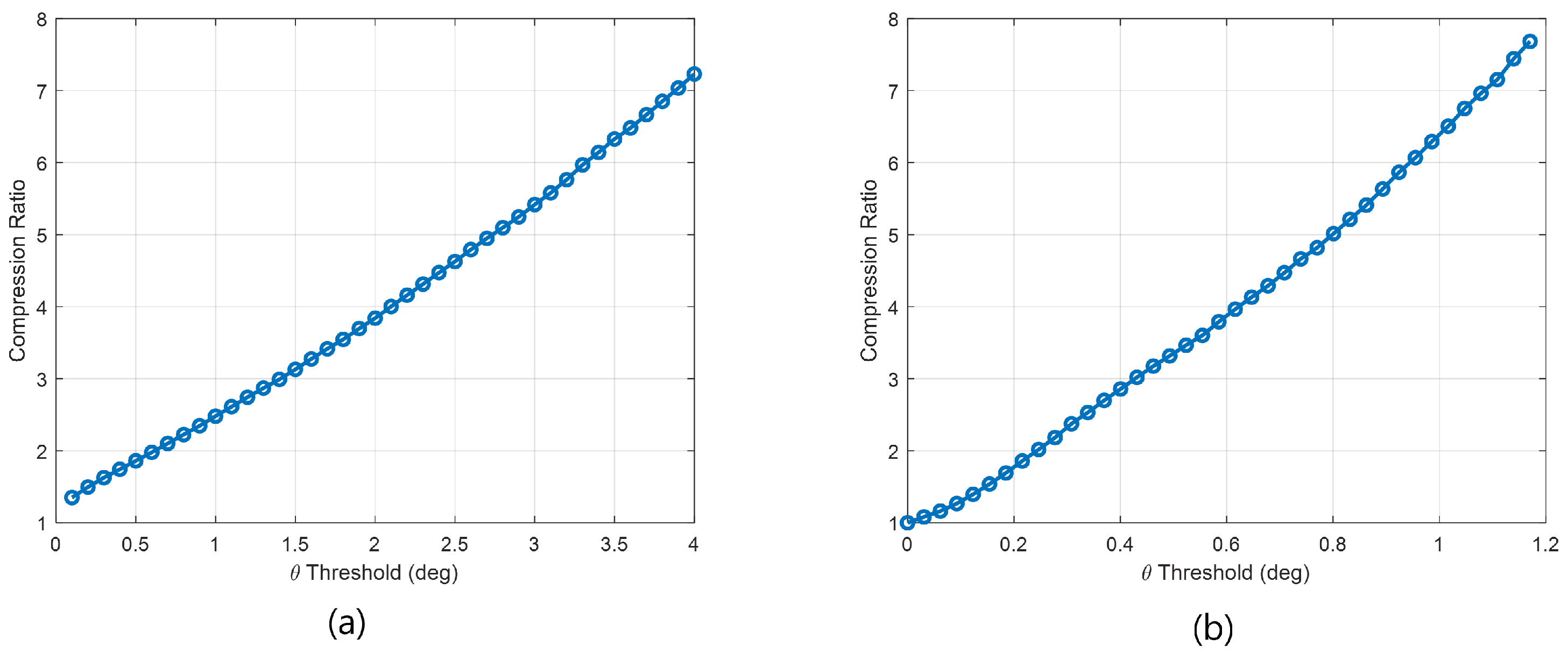
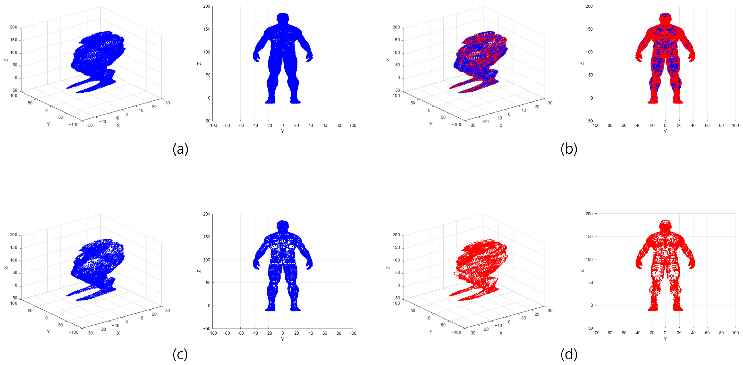
Here, $N_{\mathrm{original}}$ represents the number of original points, and $N_{\mathrm{remaining}}$ denotes the number of structural key points that were preserved (i.e., not removed) based on the given threshold $\theta$. To further investigate the influence of the angular threshold ${\theta }_{\mathrm{th}}$ on the compression performance, the compression ratio was computed across a range of threshold values by using the corresponding $N_{\mathrm{original}}$ and $N_{\mathrm{remaining}}$. The results, shown in Figure 7, demonstrate a clear trend: as ${\theta }_{\mathrm{th}}$ increases, more points are deemed structurally insignificant and consequently removed, leading to a higher compression ratio. This inverse relationship between threshold and point retention was consistently observed in both the SAR and SHREC’19 datasets, highlighting the structural sensitivity of each dataset. Figure 8 and Figure 9 illustrate the results before and after compression, respectively.

4. Experimental Results

4.1. Entropy-Based Compression Performance

The performance of the proposed structure-aware point cloud compression method was quantitatively evaluated using various metrics. To assess the degree of information preservation after compression, Shannon entropy was employed as a quantitative indicator. Entropy is an information-theoretic measure that quantifies uncertainty in a probability distribution. It can be used to indirectly evaluate how much structural information remains in the data after compression. For a 3D point cloud $X=\{x_1,x_2,\dots ,x_n\}$, the overall entropy $H\left(x\right)$ is defined based on the probability $p\left(x_i\right)$ of each point as follows:

$$H\left(x\right)=-\sum _{i=1}^{n}p\left(x_i\right)logp\left(x_i\right).$$

(16)

Here, $p\left(x_i\right)$ represents the probability density estimated using a Gaussian mixture model (GMM). Since point cloud data exhibit irregular and high-dimensional distributions, they are difficult to model using a single distribution. Therefore, in this study, we adopt a GMM, which is a linear combination of multiple Gaussian distributions, to construct the probability density function as follows:

$$p\left(x\right)=\sum _{k=1}^K{\pi }_k·\mathcal{N}(x\mid {\mu }_k,{\Sigma }_k).$$

(17)

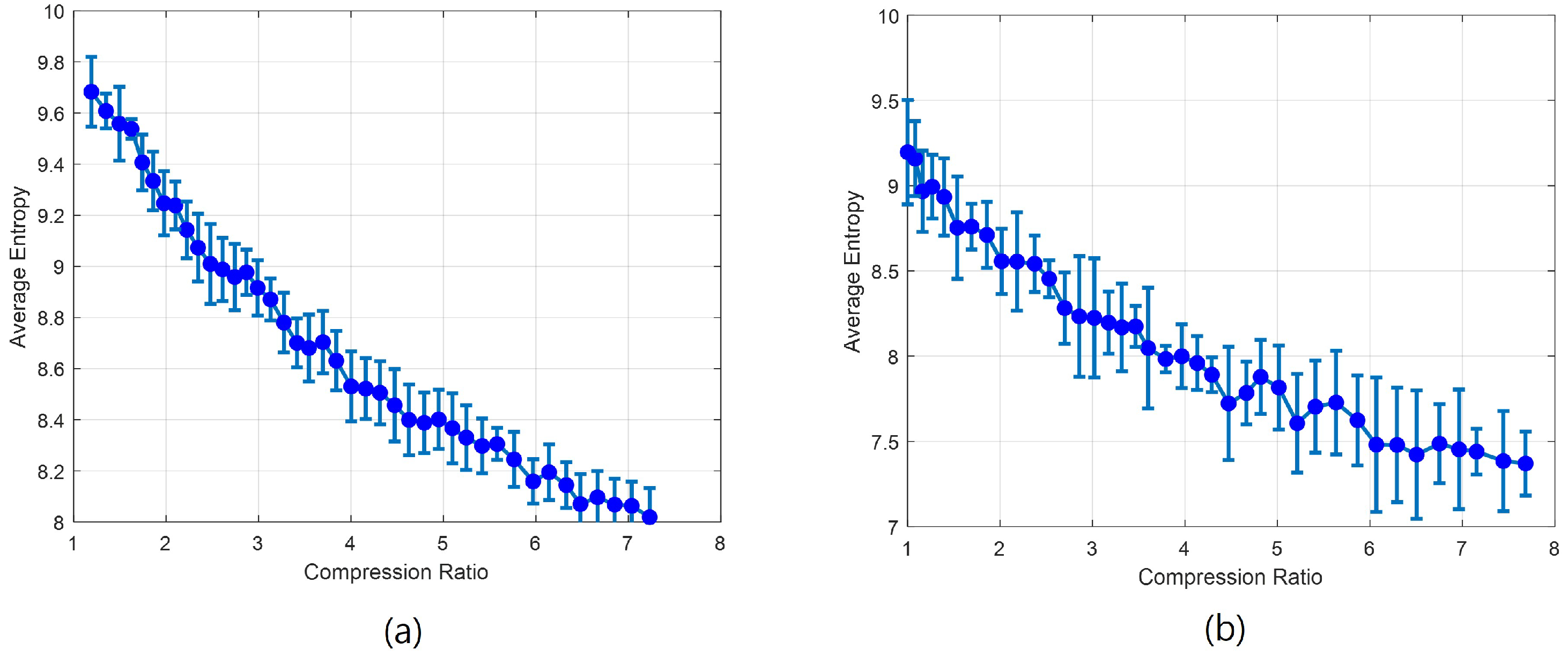
Here, K denotes the number of Gaussian components, each with a mean vector ${\mu }_k$ and a covariance matrix ${\Sigma }_k$. The mixing coefficient for each component is ${\pi }_k$, and the sum of all ${\pi }_k$ values equals 1. The probability density function of each Gaussian component is denoted as $\mathcal{N}(x\mid {\mu }_k,{\Sigma }_k)$. Based on this, the probability $p\left(x_i\right)$ for each point $x_i$ is calculated using the normalized probability density function (PDF) derived from the GMM, where the total probability density is normalized to 1. Entropy is then computed from this distribution. Compression is performed by varying the PCA-based eigenvector angular difference threshold $\theta$ from $0.1°$ to $4.0°$ in $0.1°$ increments. For each threshold $\theta$, only the points that satisfy the criterion are selectively retained, while those considered structurally less significant are progressively removed. As the compression ratio increases, the number of retained points decreases, and the corresponding changes in entropy are used to evaluate the performance of structural preservation. For each $\theta$, the experiment is repeated 10 times, and the average entropy and standard deviation are visualized. Figure 10 summarizes how average entropy varies with the compression ratio for the two datasets.

4.2. PSNR-Based Compression Performance

The peak signal-to-noise ratio (PSNR) is used as a quantitative metric to measure the similarity between the original and compressed point cloud data. The PSNR is typically expressed on a logarithmic scale as the ratio of the peak signal value to the mean squared error (MSE). A higher PSNR value indicates that the compressed data are more like the original. In this study, two distance-based criteria were used to compute PSNR. The first is the point-to-point distance. For each point $a_j$ in the original point cloud $A={\left\{a_j\right\}}_{j=1}^M$, the nearest point $b_i$ in the compressed point cloud $B={\left\{b_i\right\}}_{i=1}^N$ is found, and the Euclidean distance between the two points is calculated. Here, M and N denote the number of points in the original point cloud A and the compressed point cloud B, respectively. That is, M represents the total number of original data points before compression, and N represents the number of data points after compression. The mean squared error (MSE) is then defined as follows:

$$\mathrm{MSE}={\displaystyle \frac{1}{M}}\sum _{j=1}^M\underset{i}{min}{∥a_j-b_i∥}^2.$$

(18)

The second criterion used is the point-to-plane distance. Unlike the simple Euclidean point-to-point distance, the point-to-plane error is a more structure-sensitive quantitative metric, capable of better capturing geometric distortions. This metric is based on the method proposed by Dong Tian et al. [22]. For each point $a_j$ in the original point cloud $A={\left\{a_j\right\}}_{j=1}^M$, the nearest point $b_i$ is found in the compressed point cloud $B={\left\{b_i\right\}}_{i=1}^N$, and a local neighborhood is formed around $b_i$ to estimate the normal vector $N_j$. Then, the orthogonal (perpendicular) distance is computed based on the inner product between the vector $E(i,j)=a_j-b_i$ and the normal vector $N_j$. The mean squared error (MSE) in this case is calculated as follows:

$$\mathrm{MSE}={\displaystyle \frac{1}{M}}\sum _{j=1}^M{\left((a_j-b_i)·N_j\right)}^2.$$

(19)

In this study, the local neighborhood for estimating the surface normal was constructed using 15 points. The PSNR is then defined as follows:

$$\mathrm{PSNR}=10·{log}_{10}\left({\displaystyle \frac{p^2}{\mathrm{MSE}}}\right),$$

(20)

where p is the peak signal value in the point cloud data. Here, P is the peak value based on the maximum range of the point cloud, and it is calculated as follows:

$$P=\sqrt{{(x_{\max }-x_{\min })}^2+{(y_{\max }-y_{\min })}^2+{(z_{\max }-z_{\min })}^2}.$$

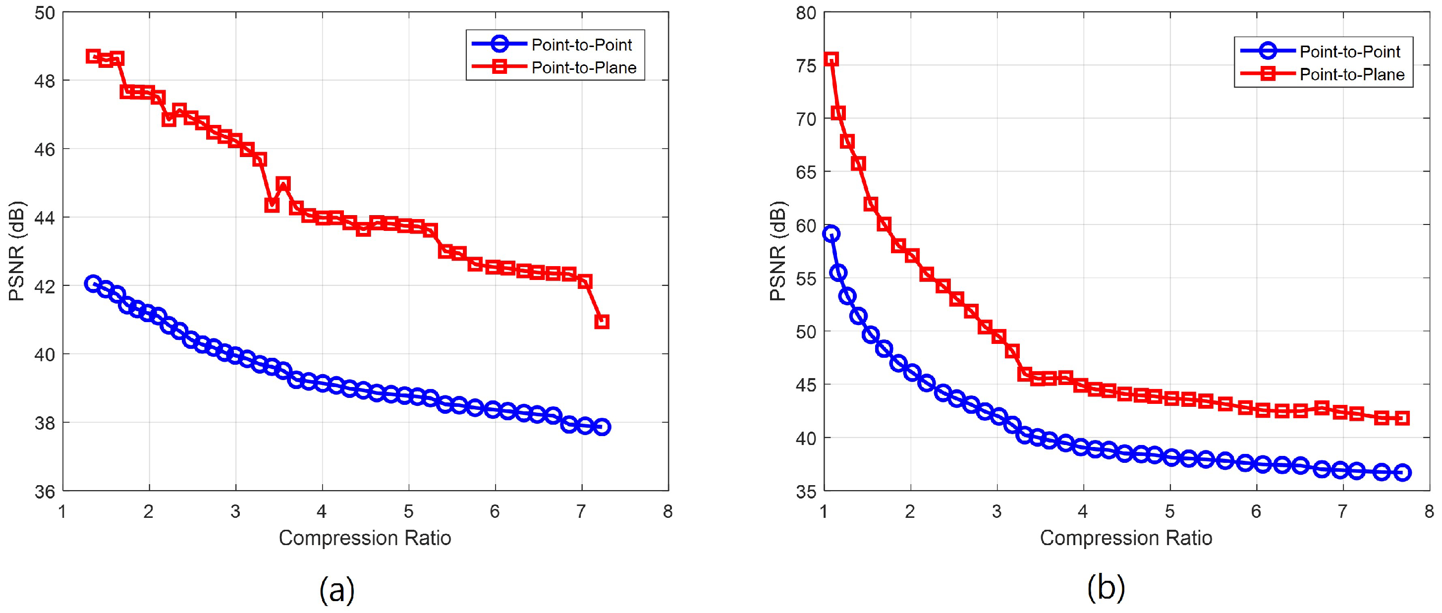
The minimum and maximum values along the x, y, and z axes are used to reflect the overall spatial extent of the original point cloud. In this study, the peak value P was set to 1.6173 for the radar dataset and 197.9034 for the SHREC’19 dataset. Figure 11 summarizes PSNR as a function of the compression ratio for the radar and SHREC’19 datasets.

4.3. SSIM-Based Compression Performance

The structural similarity index measure (SSIM) is a metric used to quantitatively evaluate the structural similarity between two images. In this study, the SSIM was employed to assess the degree of structural preservation between the original and compressed point clouds. The SSIM evaluates similarity based on three components: luminance, contrast, and structure. A value closer to 1 indicates higher structural similarity between the two datasets. To enable SSIM computation for 3D point cloud data, the point clouds were converted into 2D images through voxelization. Each point coordinate $(x,y,z)$ in the point cloud was mapped to a voxel grid location through normalization and integer transformation. In this study, the voxel size was set to 0.01 for the radar dataset and 0.1 for the SHREC’19 dataset.

$${\mathrm{Voxel}}_x=⌊{\displaystyle \frac{x}{\mathrm{voxel}\_\mathrm{size}}}⌋,{\mathrm{Voxel}}_y=⌊{\displaystyle \frac{y}{\mathrm{voxel}\_\mathrm{size}}}⌋,{\mathrm{Voxel}}_z=⌊{\displaystyle \frac{z}{\mathrm{voxel}\_\mathrm{size}}}⌋.$$

(21)

Next, 2D planar projections were performed for each plane (XY, YZ, and ZX). For each projection, a pixel value of 1 was assigned if a point existed at the corresponding location, and 0 otherwise, resulting in a binary image representation. The transformed binary images $s=s_i$ and $c=c_i$, corresponding to the source and compressed point clouds, respectively, were then used to compute the structural similarity using the following SSIM formula:

$$\mathrm{SSIM}(s,c)={\displaystyle \frac{(2{\mu }_s{\mu }_c+C_1)(2{\sigma }_{sc}+C_2)}{({\mu }_s^2+{\mu }_c^2+C_1)({\sigma }_s^2+{\sigma }_c^2+C_2)}},$$

(22)

where ${\mu }_s$ and ${\mu }_c$ are the mean values of images s and c, ${\sigma }_s^2$ and ${\sigma }_c^2$ are the variances, ${\sigma }_{sc}$ is the covariance between s and c, and $C_1$, $C_2$ are small constants to stabilize the division with weak denominators. Here, ${\mu }_s$ and ${\mu }_c$ represent the mean values of s and c, corresponding to luminance. ${\sigma }_s$ and ${\sigma }_c$ denote the variances of s and c, representing contrast. ${\sigma }_{sc}$ is the covariance between s and c, representing structural similarity. $C_1$ and $C_2$ are small constants introduced to avoid division by zero. The mean, variance, and covariance are defined as follows:

$$\begin{array}{cc}\hfill {\mu }_s& ={\displaystyle \frac{1}{N}}\sum _{i=1}^N{s}_i,{\mu }_c={\displaystyle \frac{1}{N}}\sum _{i=1}^N{c}_i,\hfill \end{array}$$

(23)

$$\begin{array}{cc}\hfill {\sigma }_s^2& ={\displaystyle \frac{1}{N}}\sum _{i=1}^N{(s_i-{\mu }_s)}^2,{\sigma }_c^2={\displaystyle \frac{1}{N}}\sum _{i=1}^N{(c_i-{\mu }_c)}^2,\hfill \end{array}$$

(24)

$$\begin{array}{cc}\hfill {\sigma }_{sc}& ={\displaystyle \frac{1}{N}}\sum _{i=1}^N(s_i-{\mu }_s)(c_i-{\mu }_c).\hfill \end{array}$$

(25)

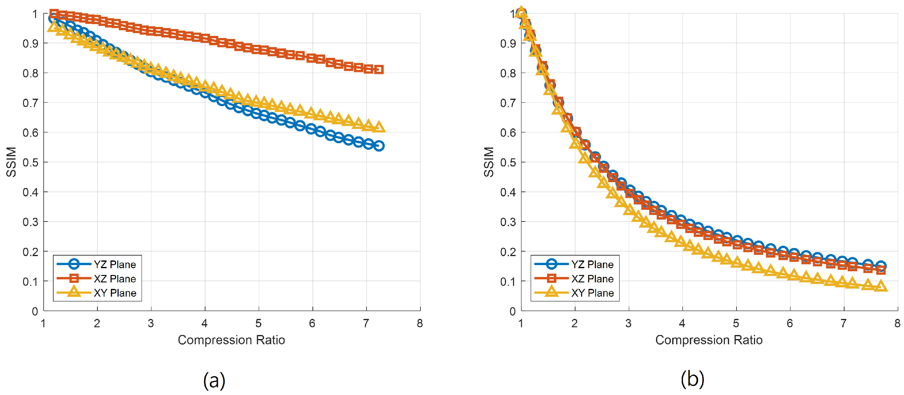
Figure 12 presents SSIM as a function of the compression ratio for the radar and SHREC’19 datasets.

4.4. Comparison of Point Cloud Compression Performance: Proposed Method vs. G-PCC

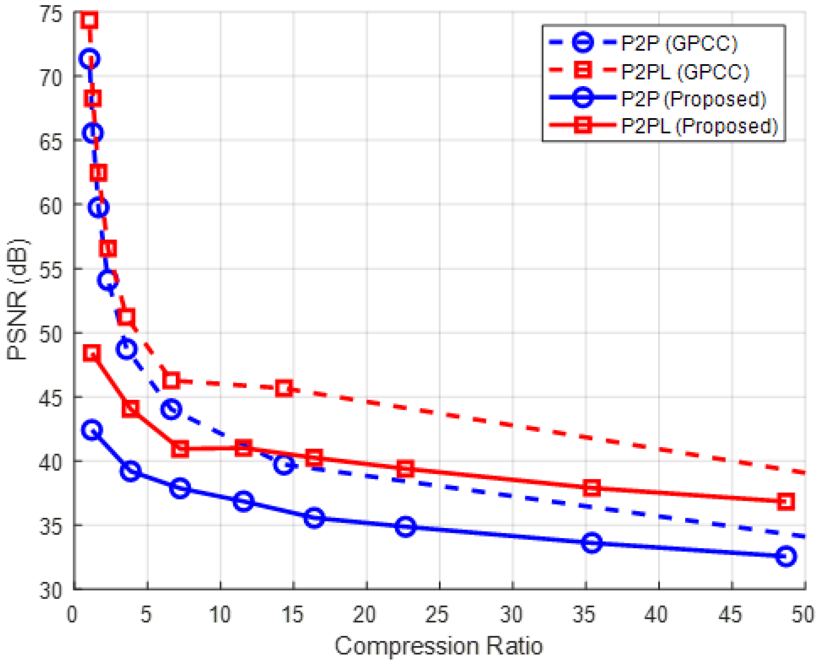
The proposed method was quantitatively compared with the conventional G-PCC compression technique on SAR data using three evaluation metrics: PSNR, entropy, and SSIM. For PSNR, two widely used metrics were considered: point-to-point (P2P), which measures the Euclidean distance between corresponding points in the original and compressed point clouds, and point-to-plane (P2PL), which evaluates the orthogonal distance from each original point to the local surface plane of the compressed point cloud. As shown in Figure 13, the PSNR of the proposed method is lower than that of G-PCC in both P2P and P2PL metrics. This is primarily because the proposed approach removes points with low structural importance, which improves the compression efficiency but may reduce point-level positional accuracy.

In the entropy comparison shown in Figure 14, both methods exhibit a decreasing trend in entropy as the compression ratio increases, indicating reduced information content. This demonstrates that the proposed method effectively removes redundant points while maintaining stable data characteristics during compression.

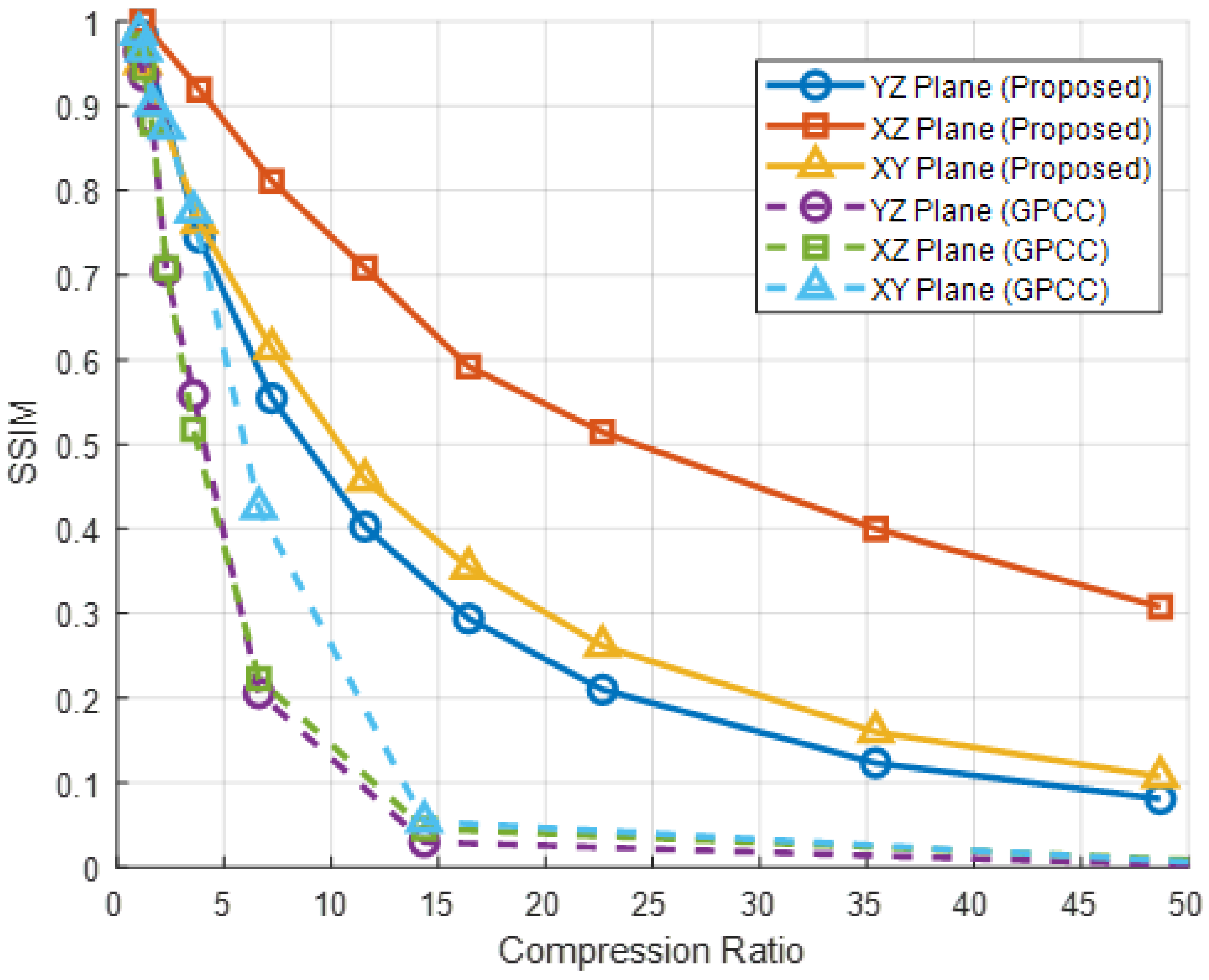
Finally, Figure 15 shows that the proposed method achieves a higher SSIM compared to G-PCC, indicating better preservation of structural similarity. By leveraging directional features of SAR point clouds, the proposed approach selectively retains points that contribute most to shape representation, resulting in improved structural fidelity.

Overall, while the proposed method shows a lower PSNR compared to G-PCC and achieves comparable performance in entropy, it demonstrates superior performance in structural similarity preservation (SSIM). This confirms its effectiveness for compressing SAR point cloud data, where maintaining shape and structural features is critical.

5. Conclusions

In this paper, we proposed a directionality-based key point preservation compression method for the efficient compression of SAR point cloud data. The proposed approach quantitatively evaluates the importance of directionality based on the angular difference of eigenvectors for each point. By removing points with directional significance below a predefined threshold, the method achieves a high compression ratio while preserving the core structural information of the data. The experimental results demonstrated that as the threshold $\theta$ increased, the compression ratio also increased gradually. Using various quantitative metrics—entropy, PSNR, and SSIM—we evaluated both the degree of information loss and the structural preservation performance. The results confirmed that the proposed method effectively performs compression by quantitatively analyzing directionality and selectively preserving key points based on their structural contribution. Unlike conventional voxel-based G-PCC compression techniques, this method introduces a new perspective by evaluating local structural differences through directional analysis. It enables the removal of redundant data while retaining essential information. As a novel approach that leverages directionality as a structural feature in point cloud compression, the proposed technique is expected to contribute to the real-time processing and transmission of high-resolution sensor-generated 3D data.

References

1. Otepka, J.; Ghuffar, S.; Waldhauser, C.; Hochreiter, R.; Pfeifer, N. Georeferenced Point Clouds: A Survey of Features and Point Cloud Management. ISPRS Int. J. Geo-Inf. 2013, 2, 1038–1065. [Google Scholar] [CrossRef]
2. Chen, S.; Liu, B.; Feng, C.; Vallespi-Gonzalez, C.; Wellington, C. 3D Point Cloud Processing and Learning for Autonomous Driving: Impacting Map Creation, Localization, and Perception. IEEE Signal Process. Mag. 2021, 38, 68–86. [Google Scholar] [CrossRef]
3. Cheng, Y.; Liu, Y. Person Reidentification Based on Automotive Radar Point Clouds. IEEE Trans. Geosci. Remote Sens. 2022, 60, 5101913. [Google Scholar] [CrossRef]
4. Zhang, Z.; Liu, J.; Jiang, G. Spatial and Temporal Awareness Network for Semantic Segmentation on Automotive Radar Point Cloud. IEEE Trans. Intell. Veh. 2024, 9, 3520–3530. [Google Scholar] [CrossRef]
5. Cheng, Y.; Su, J.; Jiang, M.; Liu, Y. A Novel Radar Point Cloud Generation Method for Robot Environment Perception. IEEE Trans. Robot. 2022, 38, 3754–3773. [Google Scholar] [CrossRef]
6. Sturm, C.; Wiesbeck, W. Waveform Design and Signal Processing Aspects for Fusion of Wireless Communications and Radar Sensing. Proc. IEEE 2011, 99, 1236–1259. [Google Scholar] [CrossRef]
7. Li, J.; Stoica, P.; Zheng, X. Signal Synthesis and Receiver Design for MIMO Radar Imaging. IEEE Trans. Signal Process. 2008, 56, 3959–3968. [Google Scholar] [CrossRef]
8. Brown, W.M.; Porcello, L.J. An Introduction to Synthetic-Aperture Radar. IEEE Spectr. 1969, 6, 52–62. [Google Scholar] [CrossRef]
9. Moreira, A.; Prats-Iraola, P.; Younis, M.; Krieger, G.; Hajnsek, I.; Papathanassiou, K.P. A Tutorial on Synthetic Aperture Radar. IEEE Geosci. Remote Sens. Mag. 2013, 1, 6–43. [Google Scholar] [CrossRef]
10. Garcia, D.C.; Fonseca, T.A.; Ferreira, R.U.; de Queiroz, R.L. Geometry Coding for Dynamic Voxelized Point Clouds Using Octrees and Multiple Contexts. IEEE Trans. Image Process. 2020, 29, 313–322. [Google Scholar] [CrossRef]
11. Liu, H.; Yuan, H.; Liu, Q.; Hou, J.; Zeng, H.; Kwong, S. A Hybrid Compression Framework for Color Attributes of Static 3D Point Clouds. IEEE Trans. Circuits Syst. Video Technol. 2022, 32, 1564–1577. [Google Scholar] [CrossRef]
12. Wang, J.; Zhu, H.; Liu, H.; Ma, Z. Lossy Point Cloud Geometry Compression via End-to-End Learning. IEEE Trans. Circuits Syst. Video Technol. 2021, 31, 4909–4923. [Google Scholar] [CrossRef]
13. Nguyen, D.T.; Quach, M.; Valenzise, G.; Duhamel, P. Lossless Coding of Point Cloud Geometry Using a Deep Generative Model. IEEE Trans. Circuits Syst. Video Technol. 2021, 31, 4617–4629. [Google Scholar] [CrossRef]
14. Li, D.; Ma, K.; Wang, J.; Li, G. Hierarchical Prior-Based Super Resolution for Point Cloud Geometry Compression. IEEE Trans. Image Process. 2024, 33, 1965–1976. [Google Scholar] [CrossRef] [PubMed]
15. Kim, J.; Rhee, S.; Kwon, H.; Kim, K. LiDAR Point Cloud Compression by Vertically Placed Objects Based on Global Motion Prediction. IEEE Access 2022, 10, 15298–15310. [Google Scholar] [CrossRef]
16. Sheng, X.; Li, L.; Liu, D.; Xiong, Z. Attribute Artifacts Removal for Geometry-Based Point Cloud Compression. IEEE Trans. Image Process. 2022, 31, 3399–3413. [Google Scholar] [CrossRef]
17. Wu, X.; Zhang, P.; Wang, M.; Chen, P.; Wang, S.; Kwong, S. Geometric Prior Based Deep Human Point Cloud Geometry Compression. IEEE Trans. Circuits Syst. Video Technol. 2024, 34, 8794–8807. [Google Scholar] [CrossRef]
18. Jung, C.; Yoo, Y.; Kim, H.-W.; Shin, H.-C. Detecting Sleep-Related Breathing Disorders Using FMCW Radar. J. Electromagn. Eng. Sci. 2023, 23, 437–445. [Google Scholar] [CrossRef]
19. Yoo, Y.-K.; Jung, C.-W.; Shin, H.-C. Unsupervised Detection of Multiple Sleep Stages Using a Single FMCW Radar. Appl. Sci. 2023, 13, 4468. [Google Scholar] [CrossRef]
20. Marin, R.; Melzi, S.; Castellani, U.; Rodolà, E. FARM: Functional Automatic Registration Method for 3D Human Bodies. arXiv 2019, arXiv:1807.10517. [Google Scholar] [CrossRef]
21. Loper, M.; Mahmood, N.; Romero, J.; Pons-Moll, G.; Black, M.J. SMPL: A Skinned Multi-Person Linear Model. ACM Trans. Graph. 2015, 34, 248:1–248:16. [Google Scholar] [CrossRef]
22. Tian, D.; Ochimizu, H.; Feng, C.; Cohen, R.; Vetro, A. Geometric Distortion Metrics for Point Cloud Compression. In Proceedings of the 2017 IEEE International Conference on Image Processing (ICIP), Beijing, China, 17–20 September 2017; pp. 346–350. [Google Scholar]
Figure 1. Linear stage system.
Applsci 15 08925 g001
Figure 2. Signal processing flowchart for radar-based point cloud generation.
Applsci 15 08925 g002
Figure 3. Merging process after Y-axis correction of point clouds for each scan.
Applsci 15 08925 g003
Figure 4. (a) Neighbor point set N i excluding the reference point p i ; (b) Augmented point set N i p including p i . Colors: reference point (red), neighbors (blue).
Applsci 15 08925 g004
Figure 5. (a) Principal eigenvector v 1 of N i (excluding p i ); (b) Principal eigenvector v 1 p of N i p (including p i ); (c) Angular difference θ between v 1 and v 1 p . Colors: reference point (red), neighbors (blue).
Applsci 15 08925 g005
Figure 6. Experimental setup. (a) Overview of the linear-stage measurement scene.; (b) Acquisition geometry showing the sensor tilted upward by 15 ° and the subject positioned at 3.0 m .
Applsci 15 08925 g006
Figure 7. Relationship between angular threshold ( θ th ) and compression ratio: (a) radar-based SAR data; (b) SHREC’19 mesh data.
Applsci 15 08925 g007
Figure 8. Visualization of radar point cloud before and after compression. (a) Full point cloud before compression; (b) overlay comparison of key points (in red) and removable points (in blue) before compression; (c) removable points after compression; (d) preserved key points after compression.
Applsci 15 08925 g008
Figure 9. Visualization of SHREC’19 mesh point cloud before and after compression. (a) Full point cloud before compression; (b) overlay comparison of key points (in red) and removable points (in blue) before compression; (c) removable points after compression; (d) preserved key points after compression.
Applsci 15 08925 g009
Figure 10. (a) Change in average entropy with respect to compression ratio (radar-based data); (b) change in average entropy with respect to compression ratio (SHREC’19 dataset).
Applsci 15 08925 g010
Figure 11. (a) PSNR according to compression ratio for radar data; (b) PSNR according to compression ratio for SHREC’19 data.
Applsci 15 08925 g011
Figure 12. (a) SSIM variation according to compression ratio for radar data. (b) SSIM variation according to compression ratio for SHREC’19 data.
Applsci 15 08925 g012
Figure 13. PSNR comparison between the proposed method and G-PCC on radar data.
Applsci 15 08925 g013
Figure 14. Entropy comparison between the proposed method and G-PCC on radar data.
Applsci 15 08925 g014
Figure 15. SSIM comparison between the proposed method and G-PCC on radar data.
Applsci 15 08925 g015