Rank-Restricted Hierarchical Alternating Least Squares Algorithm for Matrix Completion with Applications

Abstract

The matrix completion problem aims to recover missing entries in a partially observed matrix by approximating it with a low-rank structure. The two common approaches—the singular value thresholding and matrix factorization with alternating least squares—often become prohibitively expensive for large matrices or when rigorous accuracy is demanded. To address these issues, we propose a rank-restricted hierarchical alternating least squares with orthogonality and sparsity constraints, which includes a novel shrinkage function. Specifically, for faster execution speed, truncated factor matrices are updated to restrict the costly shrinkage step as well as boundary-condition heuristics. Experiments on image completion and recommender systems show that the proposed method converges with extremely fast execution speed while achieving comparable or superior reconstruction accuracy relative to state-of-the-art matrix completion methods. For example, in the image completion problem, the proposed algorithm produced outputs approximately 15 times faster on average than the most accurate reference algorithm, while achieving 98% of its accuracy.

1. Introduction

The matrix completion problem, which aims to recover missing or corrupted entries in a partially observed matrix, arises in various fields, such as recommender systems [1,2], computer vision [3,4,5], machine learning [6,7,8], and signal processing [9,10,11]. However, filling in the missing entries of a matrix is challenging because it is inherently ill-posed, as infinitely many completion results may exist. To address this issue, constraints are typically imposed on the complete matrix to capture its inherent structure or regularity. A common constraint is that the underlying matrix is of low rank, meaning that only a few linearly independent latent factors can be used to approximate the missing entries. This assumption is natural in many real-world scenarios. For example, in movie recommender systems, users’ preferences are often explained by only a few underlying factors, such as genres, actors, or directors. This low-rank property makes the matrix completion problem tractable, as it significantly reduces the degrees of freedom. Another important challenge is scalability. In real-world applications, the data matrices to be completed are often extremely large. Even though the data matrix is sparse, matrix completion algorithms typically need to perform computations on the entire matrix to recover the missing entries, requiring prohibitively expensive computational resources. Given the importance of matrix completion in practical applications, numerous methods have been developed to solve the low-rank matrix completion problem, which include optimization-based approaches and machine learning algorithms [6,7,8]. Furthermore, computationally more efficient algorithms have been extensively studied to handle large-scale data matrices [12,13].

In this paper, we focus on enhancing the performance of matrix completion by proposing a novel optimization algorithm and providing proofs of its performance in popular applications, such as image completion and recommender systems. The remainder of this paper is organized as follows. In Section 2, we introduce popular low-rank matrix completion algorithms and highlight our contributions. In Section 3, we propose a new rank-restricted hierarchical alternating least squares algorithm for matrix completion. Section 4 presents an evaluation of the numerical performance of the proposed algorithm using image completion and recommender system data. We conclude with a discussion in Section 5.

2. Related Works and Our Contribution

The mathematical expression of the low-rank completion problem is as follows: Assume that an incomplete matrix $M\in {\mathbf{R}}^{m\times n}$ is given whose observed entries are indexed by the set $\mathsf{\Omega }=\left\{(i,j)\right|M_{ij}\mathrm{is}\mathrm{observed}\}$. Matrix completion problems aim to obtain the low-rank matrix $X\in {\mathbf{R}}^{m\times n}$ that matches M on the observed positions by solving the optimization problem [14]:

$$\arg {\min }_X\mathrm{rank}\left(X\right)\mathrm{s}.\mathrm{t}.X_{ij}=M_{i,j},\forall (i,j)\in \mathsf{\Omega }.$$

(1)

Introducing the sampling operator $P_{\mathsf{\Omega }}\left(G\right)$ for any matrix G, defined by

$$P_{\mathsf{\Omega }}{\left(G\right)}_{ij}=\{\begin{array}{c}{g}_{ij}\mathrm{if}(i,j)\in \mathsf{\Omega },\hfill \\ 0\mathrm{otherwise},\hfill \end{array}$$

(2)

the problem (1) can be rewritten as

$$\arg {\min }_X\mathrm{rank}\left(X\right)\mathrm{s}.\mathrm{t}.P_{\mathsf{\Omega }}\left(X\right)=P_{\mathsf{\Omega }}\left(M\right).$$

(3)

Unfortunately, direct rank minimization in (3) is an NP-hard [15]. As a result, it requires a close approximation to rank minimization, which relaxes the problem in (3). For example, $l_1$ norm or nuclear norm relaxation have been studied [12,14,16,17]. Candès et al. [14] introduced a convex relaxation of the non-convex problem in (3) by employing nuclear norm regularization, such that

$$\arg {\min }_X{\left|\right|X\left|\right|}_{*}\mathrm{s}.\mathrm{t}.P_{\mathsf{\Omega }}\left(X\right)=P_{\mathsf{\Omega }}\left(M\right),$$

(4)

and showed that the optimal solution of (4) is equivalent to solving the following problems iteratively, such that

$$\{\begin{array}{c}{\overline{X}}_k=\mathrm{shrink}(X_k,\tau ),\hfill \\ X_{k+1}=X_k+\delta P_{\mathsf{\Omega }}(M-{\overline{X}}_k),\hfill \end{array}$$

(5)

where $\delta$ indicates the step length, k represents the iteration step, and the function $\mathrm{shrink}(X_k,\tau )$ is the soft singular value thresholding (SVT) operator with the predefined threshold value $\tau$. Inspired by the work of SVT, several methods based on nonlinear SVT algorithms have been proposed [12,18,19,20].

The method proposed by Candès et al. provided rigorous mathematical derivations of the problems and yielded excellent low-rank approximation of M. However, it demands substantial computational resources because it requires a singular value decomposition (SVD) in every iteration. To alleviate this burden, alternating minimization-based matrix factorization techniques have been explored. Assuming that the rank $r\ll \min (m,n)$ of X is known, one seeks two factor matrices $A\in {\mathbf{R}}^{m\times r}$ and $B\in {\mathbf{R}}^{n\times r}$ from M that minimize

$$\arg {\min }_{A,B}{\parallel P_{\mathsf{\Omega }}\left(M\right)-P_{\mathsf{\Omega }}\left(A{B}^T\right)\parallel }_F^2.$$

(6)

A basic alternating minimization scheme updates one factor matrix while fixing the other, such that

$$\begin{array}{cc}\hfill A_{k+1}& =\arg {\min }_A{\parallel P_{\mathsf{\Omega }}\left(M\right)-P_{\mathsf{\Omega }}\left(A{B}_k^T\right)\parallel }_F,\hfill \\ \hfill B_{k+1}& =\arg {\min }_B{\parallel P_{\mathsf{\Omega }}\left(M\right)-P_{\mathsf{\Omega }}\left(A_k{B}^T\right)\parallel }_F.\hfill \end{array}$$

(7)

Tanner and Wei proposed an alternating steepest-descent method to solve (7), which iteratively updates A and B using the steepest descent [13]. Hastie et al. [21] considered a nuclear norm-based matrix completion algorithm combined with the matrix factorization method, based on the following equation:

$${\left|\right|X\left|\right|}_{*}=\arg {\min }_{A,B,X=A{B}^T}{\displaystyle \frac{1}{2}}\left({\parallel A\parallel }_F^2+{\parallel B\parallel }_F^2\right).$$

(8)

Equation (8) implies that the nuclear norm of a matrix can be approximated by the sum of the Frobenius norms of its factor matrices. By substituting (8) into their matrix completion formulation, Hastie et al. obtained

$$\arg {\min }_X\left({\parallel A\parallel }_F^2+{\parallel B\parallel }_F^2\right)\mathrm{s}.\mathrm{t}.P_{\mathsf{\Omega }}\left(A{B}^T\right)=P_{\mathsf{\Omega }}\left(M\right).$$

(9)

Subsequently, they employed alternating minimization techniques to determine the optimal factor matrices A and B. Since solving (9) does not require an SVD, and the sizes of the factor matrices are smaller than that of X, the algorithm is expected to run faster than SVT in (5). However, the algorithm proposed by Hastie et al. is highly dependent on an accurate estimate of the rank; an incorrect value can cause the loss of crucial low-rank information or unnecessary increases in computational time. Later, Yang et al. and Li et al. proposed non-negative matrix-factorization algorithms with an adaptive graph to mitigate sensitivity to noise or outliers [22,23]. Xu et al. combined rank-1 matrix completion with an adaptive local filter to simultaneously incorporate local information and low-rank features [24]. Specifically, Xu et al. incrementally added dominant singular triplets to X and integrated it with locally filtered outputs to obtain the completed matrix. Xiao et al. proposed the tight-and-flexible rank (TFR) function—a tunable non-convex surrogate that hugs the true rank more closely than existing convex or non-convex penalties—and integrated it into a proximal alternating minimization algorithm [17]. Depending on the data characteristics, deep learning based matrix completion approaches can be also considered [6,8,25]. Specifically, deep learning-based methods offer significant advantages for highly sparse, nonlinear, and complex data matrices compared with the matrix factorization approaches introduced in this section.

This study concentrates on computing an accurate low-rank approximation of the incomplete matrix while maintaining computational efficiency. To attain this goal, a rank-restricted hierarchical alternating least squares algorithm with orthogonality and sparsity constraints is proposed. Specifically, the main contributions of the proposed algorithm are as follows:

• A novel optimal relaxation of (3) that enforces adjustable sparsity and incorporates an orthogonality constraint is proposed, yielding more accurate and computationally efficient results than the procedure in (9). Specifically, the orthogonality constraint is included to enhance computational efficiency, while a new shrinkage function is derived to enforce sparsity in the solution.
• To improve the computational efficiency within a single iteration, we employ hierarchical alternating minimization to the proposed model, enabling faster computation through column-wise updates rather than full-matrix updates. This method remains effective even with a relatively rough estimate of the rank and is faster than the procedure in (7).

3. Rank-Restricted Hierarchical Alternating Least Squares Algorithm

In this section, an efficient matrix completion algorithm, which employs hierarchical alternating least squares, is proposed. Also, orthogonality and sparsity constraints are incorporated to improve the accuracy of the matrix completion problem.

3.1. Rank-Restricted Hierarchical Alternating Least Squares with Orthogonality Constraint

Here, the hierarchical alternating least squares algorithm for the matrix completion problem is derived. Consider the matrix completion problem in (4). By substituting (8) into (4), the Lagrange multiplier equation of (4) is given as follows:

$$\mathcal{L}(A,B,\lambda )=\parallel P_{\mathsf{\Omega }}\left(M\right)-P_{\mathsf{\Omega }}\left(A{B}^T\right){\parallel }_F^2+{\lambda (\parallel A\parallel }_F^2+{\parallel B\parallel }_F^2),$$

(10)

where $\lambda$ represents the Lagrange multiplier. Because the factor matrices $A\in {\mathbf{R}}^{m\times r}$ and $B\in {\mathbf{R}}^{n\times r}$ can be interpreted as $U\mathsf{\Sigma }$ and V, respectively, where $X=U\mathsf{\Sigma }{V}^T$ denotes the SVD of X, it is reasonable to impose the orthogonality constraint on B in (10), such that

$$\mathcal{L}(A,B,\lambda ,\gamma )=\parallel P_{\mathsf{\Omega }}\left(M\right)-P_{\mathsf{\Omega }}\left(A{B}^T\right){\parallel }_F^2+{\lambda (\parallel A\parallel }_F^2+{\parallel B\parallel }_F^2)+\gamma \parallel I_r-B^T{B\parallel }_F^2,$$

(11)

where a matrix $I_r\in {\mathbf{R}}^{r\times r}$ denotes the identity matrix and $\gamma$ represents another Lagrange multiplier [26,27]. The orthogonality constraint encourages B to be orthogonal, an assumption used in the derivation of the proposed low-rank optimal relaxation method; details are provided in Section 3.2.

Remark 1.

The orthogonality constraint in (11) does not strictly enforce orthogonality; rather, it helps to avoid the zero-lock problem, which can cause intermediate results to stall at zero values and lead to convergence to a suboptimal solution [28]. Therefore, the orthogonality constraint on (11) employs an adjustable degree of orthogonality to impose a relaxed constraint on B. The Supplementary Materials present experimental results demonstrating the role of the constraint by comparing the number of iterations required for convergence with and without the constraint.

Instead of directly computing the optimal solution of (11) using the classical alternating least squares method, we employ the hierarchical least squares technique to avoid matrix inversions [29]. Let $A=[{\mathbf{a}}_1,{\mathbf{a}}_2,\dots ,{\mathbf{a}}_r]$ and $B=[{\mathbf{b}}_1,{\mathbf{b}}_2,\dots ,{\mathbf{b}}_r]$. The column-wise minimization of (11) can be written as follows:

$$\begin{array}{cc}\hfill \mathcal{L}(A,B,\lambda ,\gamma )& =\parallel P_{\mathsf{\Omega }}(M-\sum _{i=1}^r{\mathbf{a}}_i{\mathbf{b}}_i^T){\parallel }_F^2+\lambda \left[\sum _{i=1}^r\left(\parallel {\mathbf{a}}_i{\parallel }_2^2+{\parallel {\mathbf{b}}_i\parallel }_2^2\right)\right]\hfill \\ \hfill & +\gamma \left[\sum _{j=1}^r\sum _{i=1}^r\parallel {\mathbf{b}}_i^T{\mathbf{b}}_j{\parallel }_2^2-2\sum _{i=1}^r{\parallel {\mathbf{b}}_i\parallel }_2^2+r\right].\hfill \end{array}$$

(12)

The optimal solution of the column-wise minimization in (12) is obtained by taking derivatives with respect to each column ${\mathbf{a}}_i$ and ${\mathbf{b}}_i$ for $1\le i\le r$ in an alternating manner. For instance, the optimal i-th columns ${\mathbf{a}}_i$ and ${\mathbf{b}}_i$ are obtained by solving the alternating least squares method derived from (12), such that

$$\begin{array}{cc}\hfill {\mathbf{a}}_i& =\alpha M_i{\mathbf{b}}_i,\hfill \\ \hfill {\mathbf{b}}_i& =\beta M_i^T{\mathbf{a}}_i,\hfill \end{array}$$

(13)

where $M_i=M-A{B}^T+{\mathbf{a}}_i{\mathbf{b}}_i^T$, and the constants $\alpha$ and $\beta$ in (13) are defined as

$$\begin{array}{cc}\hfill \alpha & ={\displaystyle \frac{1}{({\mathbf{b}}_i^T{\mathbf{b}}_i+\lambda )}},\hfill \\ \hfill \beta & ={\displaystyle \frac{1}{({\mathbf{a}}_i^T{\mathbf{a}}_i+\lambda +\gamma \parallel I_r-B^{T}B{\parallel }_F)}}.\hfill \end{array}$$

(14)

For large-scale matrix completion problems, a further reduction in computational cost is crucial. To this end, a factor-by-factor procedure is preferred to the column-by-column procedure in (13), which is more beneficial for modern parallel computer architecture. Consequently, the updates for ${\mathbf{a}}_i$ and ${\mathbf{b}}_i$ can be obtained as

$$\begin{array}{cc}\hfill {\mathbf{a}}_i& \leftarrow \alpha M_i{\mathbf{b}}_i=\alpha ({\left[MB\right]}_i-A{\left[B^{T}B\right]}_i+{\mathbf{a}}_i{\mathbf{b}}_i^T{\mathbf{b}}_i)\hfill \\ \hfill {\mathbf{b}}_i& \leftarrow \beta M_i^T{\mathbf{a}}_i=\beta ({\left[M^{T}A\right]}_i-B{\left[A^{T}A\right]}_i+{\mathbf{b}}_i{\mathbf{a}}_i^T{\mathbf{a}}_i),\hfill \end{array}$$

(15)

where the matrix operations in (15) can be pre-computed. The detailed procedure of this algorithm is described in the following section.

3.2. Sparsity Constraint and Imposing the Boundary Condition

In this section, we discuss some performance improvement techniques for the proposed algorithm. One technique is to incorporate a sparsity constraint. The sparsity constraint enhances the quality of image denoising or filtering [30,31], and it is an essential prerequisite for recommender system problems [1]. Specifically, rather than using the truncation of the SVD of A with a predefined threshold, it is reasonable to enforce sparsity by applying a suitable nonlinear element-wise projection or filtering function known as a shrinkage function with a same threshold because the missing entries of the incomplete matrix act like sparse, high-magnitude noise when constructing $A{B}^T$. In this regard, we propose a novel shrinkage function for the sparsity constraint in the matrix completion problem.

Consider the optimization problem of the surrogate function obtained from (10), defined as follows:

$$f_{\mu ,p}(A,B)={\displaystyle \frac{1}{p}}\parallel A{B}^T{-M\parallel }_F^p+{\displaystyle \frac{\mu }{p}}{(\parallel A\parallel }_F^p+{\parallel B\parallel }_F^p),$$

(16)

for some fixed $\mu >0$. Then, the optimal solution to the matrix completion problem with a sparsity constraint can be obtained by solving

$$\arg \min f_{\mu ,p}(A,B),\mathrm{subject}\mathrm{to}{P}_{\mathsf{\Omega }}\left(M\right)=P_{\mathsf{\Omega }}\left(A{B}^T\right).$$

(17)

Proposition 1.

Let $A=U\mathsf{\Sigma }$ under the assumption in the previous section. Then, the solution of $f_{\mu ,p}(A,B)$ is obtained by applying the shrinkage operator ${\mathcal{D}}_{\gamma }(\mathsf{\Sigma },\tau ,d)$ to X, which is defined as

$${\mathcal{D}}_{\gamma }(\mathsf{\Sigma },\tau ,d)={\displaystyle \frac{{\sigma }_i^{d+1}}{{\sigma }_i^d+\tau }},$$

(18)

where ${\sigma }_i,1\le i\le r$ is the i-th element of the diagonal matrix Σ, $\tau =\sqrt[p-1]{\mu }$, and $d={\displaystyle \frac{p}{p-1}}$.

Proof. 

Taking the derivative of $f_{\mu ,p}(A,B)$ with respect to B while keeping A fixed yields

$${\displaystyle \frac{\partial f_{\mu ,p}(A,B)}{\partial B}}=A^T{(A{B}^T-M)}^{p-1}+\mu {\left(B^T\right)}^{p-1}=0.$$

(19)

Rearranging (19) and taking the $(p-1)$-th root to the equation gives

$$\begin{array}{cc}\hfill & {\left(A^T\right)}^{{\displaystyle \frac{1}{p-1}}}(A{B}^T-M)+\sqrt[p-1]{\mu }{B}^T\hfill \\ \hfill & =\left[{\left(A^T\right)}^{{\displaystyle \frac{1}{p-1}}}A+\sqrt[p-1]{\mu }I\right]B^T-{\left(A^T\right)}^{{\displaystyle \frac{1}{p-1}}}M=0.\hfill \end{array}$$

(20)

Hence,

$$B^T={\left[\tau I+{\left(A^T\right)}^{{\displaystyle \frac{1}{p-1}}}A\right]}^{-1}{\left(A^T\right)}^{{\displaystyle \frac{1}{p-1}}}M,$$

(21)

where $\tau =\sqrt[p-1]{\mu }$. Let $\mathsf{\Sigma }=\mathrm{diag}({\sigma }_1,\dots ,{\sigma }_r)$ and $U=[{\mathbf{u}}_1,\dots ,{\mathbf{u}}_r]$. If we rewrite (21) as a sum of vectors such that

$$B^T=\left[\sum _{i=1}^r{\displaystyle \frac{{\sigma }_i^{\frac{1}{p-1}}}{\tau +{\sigma }_i^{\frac{1}{p-1}}{\sigma }_i}}{\mathbf{u}}_i^T\right]M,$$

(22)

then X is obtained by

$$X=A{B}^T=\left[\sum _{i=1}^r{\mathbf{u}}_i{\displaystyle \frac{{\sigma }_i^d}{\tau +{\sigma }_i^d}}{\mathbf{u}}_i^T\right]M.$$

(23)

Let the SVD of M be $M=Z\mathsf{\Phi }{W}^T$, where $Z=[{\mathbf{z}}_1,\dots ,{\mathbf{z}}_r]$, $\mathsf{\Phi }=\mathrm{diag}[{\varphi }_1,\dots ,{\varphi }_r]$, and $W=[{\mathbf{w}}_i,\dots ,{\mathbf{w}}_r]$. Because we assumed earlier in this section that $X\approx M$, we can assume that ${\mathbf{u}}_i\approx {\mathbf{z}}_i$, ${\sigma }_i\approx {\varphi }_i$, and ${\mathbf{w}}_i\approx {\mathbf{b}}_i$ for $1\le i\le r$. Thus, X is computed as

$$X\approx \sum _{i=1}^r{\mathbf{u}}_i{\displaystyle \frac{{\sigma }_i^{d+1}}{{\sigma }_i^d+\tau }}{\mathbf{b}}_i^T.$$

(24)

Therefore, based on (24), the solution of $f_{\mu ,p}(A,B)$ is obtained by applying the shrinkage operator defined in (18), and that completes the proof.    □

Proposition 2.

The solution of (17) can be obtained by solving the two following equations alternatingly:

$$\left\{\begin{array}{c}{X}_k={\overline{\mathcal{D}}}_{\gamma }(Y_{k-1},\tau ,d)\hfill \\ Y_k=Y_{k-1}+\delta P_{\mathsf{\Omega }}(M-X_k),\hfill \end{array}\right.$$

(25)

where δ is the step length, ${\overline{\mathcal{D}}}_{\gamma }\left(Y_{k-1}\right)$ is defined as

$${\overline{\mathcal{D}}}_{\gamma }(Y_{k-1},\tau ,d)=U_{k-1}\overline{\mathsf{\Sigma }}{B}_{k-1}^T,$$

(26)

and $\overline{\mathsf{\Sigma }}$ is the diagonal matrix obtained from (18) with predefined τ and d.

Proof. 

See [14].    □

Remark 2.

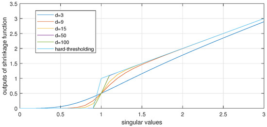
The shrinkage function (18) sharply filters out the small singular values ${\sigma }_i$,

$$D_{\gamma }(\mathsf{\Sigma },\tau ,d)={\displaystyle \frac{{\sigma }_i}{\frac{\tau }{{\sigma }_i^d}+1}}\approx 0,$$

when d is sufficiently large. Contrarily, for large singular values, since ${\displaystyle \frac{\tau }{{\sigma }_i^d}}\approx 0$, $D_{\gamma }(\mathsf{\Sigma },\tau ,d)\approx {\sigma }_i$. Figure 1 shows this behavior for singular values uniformly distributed in $[0,3]$; as d increases, the curve approaches that of the Iterative Hard Thresholding (IHT) operator, which enforces sparsity to the results [32].

Figure 1. Shrinkage function with different d.

The proposed hierarchical alternating least squares minimization algorithm for the matrix completion problem (HALMC) is summarized in Algorithm 1, and Figure 2 provides a high-level workflow for additional clarity.

Algorithm 1  $X_{k+1}=\mathrm{HALMC}(M,\mathsf{\Omega },\gamma ,\lambda ,\delta ,\tau ,d,r,ϵ)$
1:   $X_0=P_{\mathsf{\Omega }}\left(M\right)$
2:   $A_0=U_0(:,1:r){\mathsf{\Sigma }}_0(1:r,1:r)$ and $B_0=V_0(1:r)$, where $[U_0,{\mathsf{\Sigma }}_0,V_0]=\mathrm{svd}\left(M\right)$
3:  for k = 1,2,… do
4:      $W=X_k^T{A}_k$, $Y=A_k^T{A}_k$, and compute $\beta$ defined in (14)	▷ $O\left(\right|\mathsf{\Omega }|r+m{r}^2)$
5:      for j = 1,2,…,r do
6:          ${\mathbf{b}}_j=\beta (W_j-B{Y}_j+{\mathbf{b}}_j{\mathbf{a}}_j^T{\mathbf{a}}_j)$	▷ $O(nr+m^2)$
7:      end for
8:      $P=X_k{B}_k,Q=B_k^T{B}_k$, and compute $\alpha$ defined in (14)	▷ $O\left(\right|\mathsf{\Omega }|r+n{r}^2)$
9:      for j = 1,2,…,r do
10:          ${\mathbf{a}}_j=\alpha (P_j-A{Q}_j+{\mathbf{a}}_j{\mathbf{b}}_j^T{\mathbf{b}}_j)$	▷ $O(mr+n^2)$
11:      end for
12:      $[U,\mathsf{\Sigma },V]=\mathrm{svd}\left(A_k\right)$	▷ $O\left(m^{2}r\right)$
13:      $\overline{\mathsf{\Sigma }}=\mathrm{shrink}(A_k,\tau ,d)$ where shrinkage operator is defined in (18)
14:      Set $A_k=U\overline{\mathsf{\Sigma }}{V}^T$	▷ $O\left(m{r}^2\right)$
15:      $X_{k+1}=X_k+\delta P_{\mathsf{\Omega }}(M-A_k{B}_k^T)$	▷ $O\left(\right|\mathsf{\Omega }\left|r\right)$
16:      if ${\displaystyle \frac{\parallel X_{k+1}-X_k{\parallel }_F^2}{\parallel X_k{\parallel }_F^2}}>ϵ$ then
17:          break
18:      end if
19:  end for
20:  return  $X_{k+1}$

Figure 2. Diagram of proposed algorithm.

Another technique is to impose a boundary condition on M as a preprocess step for HALMC. It is well known that images reconstructed from the truncation of singular values are affected by the boundary value [33]. Therefore, considering the boundary condition may improve the performance of image completion, for example, by reducing the ringing artifacts, thus saving computational resources. For a detailed mathematical formulation imposing a boundary condition on low-rank matrix recovery, readers may refer to [34,35]. For the same reason, in the recommender system application, it is possible to improve the performance of HALMC by considering the boundary condition. Typical boundary conditions include zero (i.e., Dirichlet), periodic, and reflective (i.e., Neumann) boundary conditions. Among them, the reflective boundary condition, where the entries outside the matrix form a mirror image of the interior, is preferred in many image processing applications because it prevents discontinuity near the boundary. For example, a $3\times 3$ matrix M and its reflective extension $M_{\mathrm{ext}}$ of radius 3 are

$$M=\begin{array}{|ccc|}\hline 1& 2& 3\\ 4& 5& 6\\ 7& 8& 9\\ \hline\end{array},M_{\mathrm{ext}}=\begin{array}{|ccccccccc|}\hline 9& 8& 7& 7& 8& 9& 9& 8& 7\\ 6& 5& 4& 4& 5& 6& 6& 5& 4\\ 3& 2& 1& 1& 2& 3& 3& 2& 1\\ 3& 2& 1& 1& 2& 3& 3& 2& 1\\ 6& 5& 4& 4& 5& 6& 6& 5& 4\\ 9& 8& 7& 7& 8& 9& 9& 8& 7\\ 9& 8& 7& 7& 8& 9& 9& 8& 7\\ 6& 5& 4& 4& 5& 6& 6& 5& 4\\ 3& 2& 1& 1& 2& 3& 3& 2& 1\\ \hline\end{array}$$

In this study, a reflective boundary condition is applied to each incomplete matrix before executing HALMC. Subsequently, the restored matrix is cropped back to its original size.

3.3. Computational and Memory Complexity

HALMC performs an SVD at each iteration, but the decomposition is applied to the smaller factor matrix $A_k$ rather than to $X_k$, thereby reducing computational cost. If HALMC converges at iteration k, the overall complexity is approximately $O\left(m^{2}rk\right)$ flops. Detailed operation counts appears as comments in the pseudocode. For the memory cost analysis, we assume that only the entries of X in $\mathsf{\Omega }$ are required, resulting in a cost of $O\left(\right|\mathsf{\Omega }\left|\right)$. The memory required for the intermediate factor matrices is $O\left(\right(m+n\left)r\right)$. Therefore, the total memory cost requires $O\left(\right|\mathsf{\Omega }|+(m+n\left)r\right)$.

4. Numerical Experiments

This section presents numerical experiments designed to demonstrate the efficiency and accuracy of the proposed algorithm. For performance comparison with HALMC, we evaluated the following reference algorithms: Singular Value Thresholding (SVT) [14], Modified Schatten 2/3-Norm Minimization with Reweighting (TSNMR) [12], Rank-Restricted Efficient Minimum-Margin Matrix Factorization: SoftImpute-ALS (SoftImp) proposed by Hastie et al. [21] (p. 3375), Low-Rank Matrix Completion (LAMC) proposed by Xu et al. [24], and matrix completion with Tight and Flexible Rank (TFR) proposed by Xiao et al. [17] (https://jin-liangxiao.github.io/, accessed on 1 August 2025). Note that SVT, TSNMR, and TFR focus on developing novel shrinkage functions for matrix completion, while SoftImp and LAMC employ rank-restricted matrix factorization. All experiments were implemented using MATLAB version 9.10.00.1710957. The algorithms were tested on two common applications, image completion and recommender system, and were executed on an Intel Core i9-11900K processor with 64 GB memory.

4.1. Image Completion Problem

One of the most popular applications for matrix completion problems is image completion. The image completion problem, also known as image inpainting, involves repairing defects in individual pixel values or regions of digital images caused by some dirt, a scratch, or cracks on charge-coupled device (CCD) or impulse-type noise in images [3,36]. Given the location of the contaminated pixels, these pixels are treated as missing. An intuitive approach to restore the missing pixels is to replace their values with the interpolated values from adjacent pixels. Bertalmio et al. enhanced this approach by iteratively diffusing the values from the surrounding information, which exploits the idea of the thermal diffusion equation in physics [37]. Later, the time-consuming nature of the algorithm proposed by Bertalmio et al. was further improved by considering a total variation model [38]. Another strategy for image completion involves exploiting the low-rank structure inherent in many images. Low-rank image completion algorithms predict missing pixels using a low-rank approximation of the partially observed pixels from the image matrix. In this work, we focus on reconstructing the incomplete images based on low-rank image completion methods. We also demonstrate that the proposed algorithm is effective for image completion problems. For the experiments, we used popular natural images with randomly generated missing pixels to evaluate the performance of the algorithms.

Figure 3a, Figure 4a, Figure 5a and Figure 6a depict the natural images used in our experiments. The images have dimensions of $128\times 128$, $256\times 256$, $512\times 512$, and $1024\times 1024$, respectively. To compare the performance of the algorithms, we measured execution time, the number of iterations to converge, mean-squared error (MSE), peak signal-to-noise (PSNR) values, structural similarity index measure (SSIM), and feature similarity index (FSIM) [39]. PSNR is defined as

$$\mathrm{PSNR}=20{\log }_{10}\left({\displaystyle \frac{\max \left(\overline{X}\right)}{\sqrt{\frac{1}{mn}{\sum }_{i=0}^m{\sum }_{j=0}^n{(\overline{X}(i,j)-X(i,j))}^2}}}\right),$$

(27)

and SSIM is defined as

$$\mathrm{SSIM}={\displaystyle \frac{(2\overline{\mu }\left(\overline{X}\right)\overline{\mu }\left(X\right)+c_1)(2\overline{\sigma }(\overline{X},X)+c_2)}{(2\overline{\mu }{\left(\overline{X}\right)}^2+\overline{\mu }{\left(X\right)}^2+c_1)(\overline{\sigma }{\left(\overline{X}\right)}^2+\overline{\sigma }{\left(X\right)}^2+c_2)}}.$$

(28)

In (27) and (28), $\overline{X}$ represents the original image without missing pixels, while X denotes the image reconstructed by the algorithms. The term $\overline{\mu }\left(M\right)$ denotes the average of an arbitrary matrix M, $\overline{\sigma }\left(M\right)$ denotes its variance, and $\overline{\sigma }(M,N)$ represents the covariance between two arbitrary matrices M and N. The constants $c_1$ and $c_2$ are included to stabilize the division in cases where the denominator is small. While MSE and PSNR provide basic pixel-wise error measurements, SSIM evaluates structural fidelity, and FSIM captures perceptually important features, particularly in textured regions. Therefore, higher SSIM and FSIM values, along with lower MSE and higher PSNR, indicate better perceptual and numerical similarity to the ground truth.

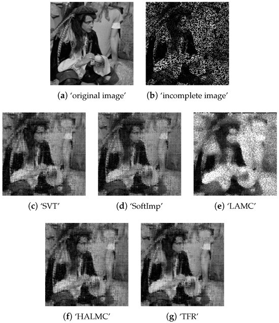
Figure 3. Experimental results of the algorithm on ‘indian’ image with 50% missing pixels.

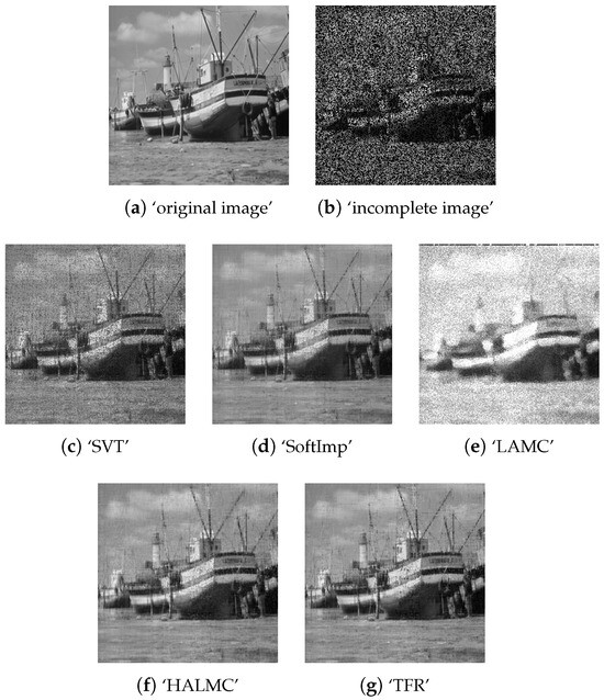
Figure 4. Experimental results of the algorithm on ‘boat’ image with 50% missing pixels.

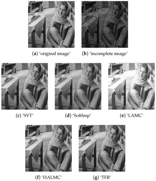
Figure 5. Experimental results of the algorithm on ‘barbara’ image with 50% missing pixels.

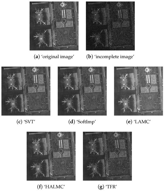
Figure 6. Experimental results of the algorithm on ‘airport’ image with 50% missing pixels.

To simulate incomplete images, we randomly selected missing pixels with various missing rates. Specifically, we randomly removed 30%, 50%, and 70% of the pixels from the entire image area and treated them as missing. To determine the optimal hyperparameters, we conducted empirical experiments by varying one hyperparameter at a time while keeping the others fixed. Based on these experiments, we set $\gamma =0.1$ defined in (12), the truncation level as $0.25m$ for both HALMC and SoftImp (where m is the size of the squared test image), $d=15$ as defined in (18), and the boundary condition to 3. For a detailed procedure of selecting the hyperparameters for HALMC, readers may refer to the Supplementary Materials.

To ensure a fair comparison among all algorithms, we define the stopping criterion as follows:

$${\displaystyle \frac{\parallel X_k-X_{k-1}{\parallel }_F^2}{\parallel X_k{\parallel }_F^2}}\le ϵ,$$

(29)

where $ϵ=1.0e-4$ is the predefined threshold. All experimental results were averaged over 20 independent trials.

Table 1, Table 2, Table 3 and Table 4 present the experimental results of all compared algorithms. To highlight the best performance, the top two results in each table are boldfaced. Since TSNMR produces meaningless output due to its inaccuracy and failure to converge, its results were excluded from the analysis. According to the experimental results, HALMC, TFR, and SVT achieved the highest visual quality across all test images and incompletion ratios. In some cases—such as ‘indian’ and ‘barbara’ under specific incompletion ratios—SVT produced highly accurate image restorations. TFR, in particular, achieved the best accuracy for the ‘indian’ image with 30% missing pixels. However, overall, the most accurate results across the experiments were achieved by HALMC. Specifically, HALMC consistently outperformed the other methods in terms of overall pixel-level differences (measured by MSE and PSNR) and structural differences (measured by SSIM and FSIM). Moreover, HALMC produced stable outputs regardless of the incompletion ratios, unlike SVT and TFR, which tended to yield less accurate results as the missing pixel rate increased. LAMC showed relatively higher FSIM values compared to the other accuracy metrics, such as MSE and PSNR. It can be interpreted that the local-filtering module in LAMC improved the local feature similarities, particularly under severe image degradation.

Table 1. Performance comparisons of the algorithms on the ‘indian’ image. The hyperparameters are set to $\lambda =1$ and $\tau =0.5$ for HALMC.

Missing Rate	Method	Iter.	Time	MSE	PSNR	SSIM	FSIM
30%	incomp.	-	-	0.2976	12.9949	0.9971	0.9468
	SVT	25.1	0.0405	0.0161	25.7045	0.9999	0.9962
	SoftImp	8.2	0.0111	0.0169	25.4353	0.9998	0.9961
	LAMC	102.6	4.7897	0.3074	13.0869	0.9953	0.9695
	HALMC	50.5	0.0245	0.0173	25.3861	0.9999	0.9954
	TFR	16.2	0.0259	0.0129	26.6635	0.9999	0.9968
50%	incomp.	-	-	0.5015	10.7283	0.9931	0.9209
	SVT	21.4	0.0364	0.0431	21.3984	0.9996	0.9888
	SoftImp	19.3	0.0184	0.0405	21.6562	0.9996	0.9894
	LAMC	99.2	4.8873	0.3030	13.1135	0.9955	0.9667
	HALMC	26.7	0.0141	0.0377	21.9917	0.9997	0.9893
	TFR	32.0	0.0504	0.0319	22.7804	0.9998	0.9911
70%	incomp.	-	-	0.69903	9.2864	0.9875	0.9016
	SVT	500.0	0.7911	0.1527	16.0030	0.9979	0.9616
	SoftImp	17.3	0.0147	0.0947	17.9690	0.9988	0.9724
	LAMC	93.0	4.7726	0.2925	13.2024	0.9957	0.9633
	HALMC	22.0	0.0112	0.0880	18.2990	0.9991	0.9729
	TFR	67.1	0.1028	0.0908	18.2937	0.9993	0.9738

Table 2. Performance comparisons of the algorithms on ‘boat’ image. The hyperparameters are set to $\lambda =1$ and $\tau =0.5$ for HALMC.

Missing Rate	Method	Iter.	Time	MSE	PSNR	SSIM	FSIM
30%	incomp.	-	-	0.2998	10.5942	0.9950	0.8889
	SVT	178.3	1.1371	0.0082	26.2113	0.9998	0.9915
	SoftImp	8.8	0.0347	0.0073	26.7184	0.9998	0.9905
	LAMC	71.7	18.7550	0.2675	11.5962	0.9928	0.9379
	HALMC	86.9	0.1484	0.0038	29.5150	0.9999	0.9959
	TFR	35.0	0.2162	0.0039	29.3969	0.9999	0.9960
50%	incomp.	-	-	0.4998	8.3751	0.9881	0.8663
	SVT	161.3	1.0556	0.0398	19.3630	0.9992	0.9625
	SoftImp	13.3	0.0481	0.0142	23.8497	0.9997	0.9819
	LAMC	66.8	18.4806	0.2593	11.6512	0.9929	0.9367
	HALMC	60.1	0.1064	0.0097	25.4886	0.9999	0.9879
	TFR	59.0	0.3657	0.0127	24.3281	0.9998	0.9850
70%	incomp.	-	-	0.6999	6.9127	0.9783	0.8561
	SVT	500.0	3.2191	0.0352	20.0334	0.9994	0.9578
	SoftImp	21.7	0.0578	0.0284	20.8240	0.9993	0.9632
	LAMC	61.4	18.7958	0.2395	11.8678	0.9931	0.9363
	HALMC	55.3	0.0458	0.0219	21.9476	0.9996	0.9689
	TFR	101.3	0.6076	0.0650	17.2651	0.9987	0.9345

Table 3. Performance comparisons of the algorithms on ‘barbara’ image. The hyperparameters are set to $\lambda =0.5$ and $\tau =0.3$ for HALMC.

Missing Rate	Method	Iter.	Time	MSE	PSNR	SSIM	FSIM
30%	incomp.	-	-	0.2998	11.1183	0.9956	0.9342
	SVT	266.5	7.8123	0.0040	29.8465	0.9999	0.9988
	SoftImp	10.4	0.1647	0.0104	25.7064	0.9998	0.9949
	LAMC	96.0	97.9771	0.2373	12.8977	0.9945	0.9772
	HALMC	22.5	0.2248	0.0072	27.3277	0.9999	0.9970
	TFR	53.5	1.4965	0.0107	25.5943	0.9999	0.9958
50%	incomp.	-	-	0.5002	8.8956	0.9895	0.9026
	SVT	248.5	7.5049	0.0114	25.3140	0.9998	0.9961
	SoftImp	17.1	0.2751	0.0189	23.1023	0.9997	0.9907
	LAMC	89.0	99.2489	0.2256	12.9940	0.9946	0.9766
	HALMC	53.0	0.5171	0.0125	24.9203	0.9998	0.9952
	TFR	189.3	5.3344	0.0154	24.1440	0.9998	0.9939
70%	incomp.	-	-	0.6998	7.4372	0.9809	0.8717
	SVT	500.0	14.0607	0.0376	20.1641	0.9994	0.9832
	SoftImp	29.0	0.3896	0.0374	20.1628	0.9992	0.9804
	LAMC	78.9	98.6612	0.2235	12.9410	0.9945	0.9745
	HALMC	18.7	0.1928	0.0368	20.2316	0.9994	0.9820
	TFR	220.1	5.9861	0.0640	17.8678	0.9991	0.9714

Table 4. Performance comparisons of the algorithms on ‘airport’ image. The hyperparameters are set to $\lambda =0.5$ and $\tau =0.1$ for HALMC.

Missing Rate	Method	Iter.	Time	MSE	PSNR	SSIM	FSIM
30%	incomp.	-	-	0.3001	14.2484	0.9978	0.9849
	SVT	500.0	68.8015	0.0125	28.0383	0.9999	0.9995
	SoftImp	12.0	1.2559	0.0173	26.6350	0.9998	0.9978
	LAMC	76.0	369.7370	0.1622	16.9316	0.9978	0.9867
	HALMC	56.1	1.8325	0.0105	28.8003	0.9999	0.9995
	TFR	72.7	10.6755	0.0137	27.6484	0.9999	0.9992
50%	incomp.	-	-	0.4997	12.0339	0.9948	0.9687
	SVT	500.0	72.2569	0.0296	24.3104	0.9998	0.9980
	SoftImp	19.0	1.7221	0.0288	24.4284	0.9997	0.9952
	LAMC	73.0	370.1930	0.1447	17.4208	0.9982	0.9872
	HALMC	54.4	1.7604	0.0191	26.2006	0.9999	0.9984
	TFR	81.0	11.9213	0.2502	15.5245	0.9981	0.9822
70%	incomp.	-	-	0.7002	10.5691	0.9905	0.9454
	SVT	500.0	71.9124	0.0523	21.8857	0.9997	0.9940
	SoftImp	29.0	2.1861	0.0494	22.0774	0.9995	0.9918
	LAMC	74.0	652.0080	0.1294	17.9027	0.9984	0.9876
	HALMC	37.0	1.2327	0.0393	23.0746	0.9997	0.9936
	TFR	82.0	11.8185	0.4199	13.2978	0.9957	0.9633

In terms of execution time, HALMC demonstrated significant efficiency while maintaining high accuracy. Although SoftImp achieved the fastest execution time, its performance degraded more rapidly as the incompletion ratio increased, specifically compared to HALMC. Overall, considering the execution time, robustness, and accuracy in image completion, HALMC emerges as the most effective algorithm among the four evaluated. Example output images generated by the algorithms for the case of 50% missing pixels are shown in Figure 3c–g, Figure 4c–g, Figure 5c–g and Figure 6c–g.

4.2. Recommender System

Another application for matrix completion problems is a recommender system. The primary goal of recommender systems is to provide personalized item recommendations to users based on their explicit or implicit preference information. Specifically, user preferences are typically estimated using ratings of similar items, indicating the user’s affinity for related items. As rating data of two entities (users and items) are often placed in matrix form, and users tend to rate only a small subset of items, estimation of the preferences can be considered as predicting missing entities from a large and sparse matrix. To address this challenge, matrix completion algorithms are extensively studied for decades. One widely adopted approach involves low-rank approximation of the rating matrix, providing an effective solution for predicting missing entries and enhancing the accuracy of recommender systems [1,2].

The low-rank matrix completion algorithms predict missing values by using the low-rank approximation of partially observed rating values in the rating matrix. Given a set of users $u\in 1,\dots ,m$ and items $i\in 1,\dots ,n$, if we let $y_{ui}$ be the rating of user u and item i, then the rating matrix $X\in {\mathbf{R}}^{m\times n}$ can be defined as

$$P_{\mathsf{\Omega }}{\left(X\right)}_{ui}=\{\begin{array}{c}{y}_{ui},\mathrm{if}(u,i)\in \mathsf{\Omega }\hfill \\ 0\mathrm{otherwise},\hfill \end{array}$$

(30)

where the set $\mathsf{\Omega }=\{(u,i)|y_{ui}\}$ is observed. Hence, the proposed low-rank matrix completion algorithm is applicable to the recommender system to fill out the missing rate values. To measure the performance of the proposed algorithm to recommender systems, we used the MovieLens 100k dataset that has a rating matrix $X\in {\mathbf{R}}^{943\times 1682}$, MovieLens 1M dataset that has a rating matrix $X\in {\mathbf{R}}^{6040\times 3952}$, and Bookcrossing dataset that has a rating matrix of size $1295\times 17,384$. The MovieLens 100k dataset has 97.48% of unrated entries, MovieLens 1M dataset has 98.32%, and Bookcrossing dataset has 99.95%. The datasets have rating values $y_{ui}$ ranging from 1 to 5 for MovieLens 100k and MovieLens 1M, and from 1 to 10 for Bookcrossing. To evaluate performance, we randomly chose 20%, 40%, and 60% of the non-zero-rating values in the datasets and considered them as missing values. After completing the rating matrices, we calculated the mean absolute error (MAE) from the ground truth data and RMSE, where MAE and root mean square error (RMSE) are defined as follows [2]:

$$\begin{array}{cc}\hfill \mathrm{MAE}& ={\displaystyle \frac{{\sum }_{u=1}^m{\sum }_{i=1}^n|P_{\overline{\mathsf{\Omega }}}\left(X^{*}\right)-P_{\overline{\mathsf{\Omega }}}\left(X\right)|}{N}},\hfill \\ \hfill \mathrm{RMSE}& =\sqrt{{\displaystyle \frac{{\sum }_{u=1}^m{\sum }_{i=1}^n{(P_{\overline{\mathsf{\Omega }}}\left(X^{*}\right)-P_{\overline{\mathsf{\Omega }}}\left(X\right))}^2}{N}}}.\hfill \end{array}$$

(31)

Here, $\overline{\mathsf{\Omega }}$ represents the set of randomly chosen missing values to be predicted, $X^{*}$ indicates the ground-truth rating matrix, and N denotes the number of missing values in $\overline{\mathsf{\Omega }}$. The lower the MAE, the closer the prediction of missing user ratings. Similarly, we empirically chose hyperparameters of the algorithm, as well as common parameters, including stopping criterion.

Table 5, Table 6 and Table 7 present the experimental results. As with the image completion experiments, SoftImp demonstrated relatively fast computation speed but yielded unsatisfactory accuracy. SVT produced highly accurate results; however, it suffered from excessive computation time, which makes it less viable for large recommender system datasets. Additionally, SVT showed limited robustness in terms of convergence. TSNMR achieved excellent accuracy across nearly all recommender system datasets, but it failed to converge within the predefined maximum number of iterations. The convergence history for TSNMR is shown in the Supplementary Materials. This resulted in prohibitively high computational costs, rendering TSNMR impractical for large-scale applications. In contrast, HALMC consistently demonstrated the best execution speed across all recommender system datasets and varying missing rates, making it well-suited for large datasets. Although HALMC did not achieve the highest accuracy in all cases, its significantly faster execution speed and reasonable accuracy make it a practical and scalable option for a recommender system.

Table 5. Performance comparisons of the algorithms on ‘Movielens 100K’ dataset. The hyperparameters are set to $\lambda =1$ and $\tau =0.5$ for HALMC.

Missing Rate	Method	Iter.	Time	MAE	RMSE
20%	incomp.	-	-	3.5280	3.7034
	SVT	210.90	30.1586	1.0732	1.2894
	SoftImp	50.00	4.3338	1.0772	1.2988
	TSNMR	500.00	88.6608	0.9778	1.1729
	HALMC	22.00	0.8978	0.9848	1.1927
	TFR	169.67	24.7094	1.1993	1.4351
40%	incomp.	-	-	3.5274	3.7032
	SVT	185.00	24.9133	1.1314	1.3569
	SoftImp	52.00	4.1866	1.1479	1.3789
	TSNMR	500.00	83.1942	1.0178	1.2298
	HALMC	22.40	0.9102	1.0152	1.2281
	TFR	162.50	23.3946	1.2675	1.5077
60%	incomp.	-	-	3.5291	3.7044
	SVT	155.20	21.0388	1.2425	1.4824
	SoftImp	56.00	4.4691	1.2589	1.5029
	TSNMR	500.00	84.1506	1.2208	1.4323
	HALMC	23.00	0.9184	1.0789	1.3025
	TFR	174.00	24.1157	1.3800	1.6268

Table 6. Performance comparisons of the algorithms on ‘Movielens 1M’ dataset. The hyperparameters are set to $\lambda =1$ and $\tau =1$ for HALMC.

Missing Rate	Method	Iter.	Time	MAE	RMSE
20%	incomp.	-	-	3.5812	3.7516
	SVT	500.00	6399.8700	1.0244	1.2265
	SoftImp	51.00	268.8490	1.2549	1.4883
	TSNMR	500.00	6860.5200	0.9359	1.1240
	HALMC	29.00	21.6903	1.0621	1.2591
	TFR	27.00	358.8730	2.6127	2.8424
40%	incomp.	-	-	3.5819	3.7519
	SVT	500.00	6401.6500	1.0884	1.2999
	SoftImp	55.00	285.1180	1.3028	1.5395
	TSNMR	500.00	6849.0600	0.9466	1.1321
	HALMC	28.50	21.6172	1.0820	1.2827
	TFR	35.00	463.2450	2.4723	2.7358
60%	incomp.	-	-	3.5813	3.7515
	SVT	434.00	5529.1200	1.1519	1.3707
	SoftImp	60.00	296.5940	1.4163	1.6599
	TSNMR	500.00	6821.0300	0.9495	1.1301
	HALMC	29.50	22.2253	1.1213	1.3269
	TFR	46.00	606.4590	2.4454	2.6799

Table 7. Performance comparisons of the algorithms on ‘Bookcrossing’ dataset. The hyperparameters are set to $\lambda =1$ and $\tau =1$ for HALMC.

Missing Rate	Method	Iter.	Time	MAE	RMSE
20%	incomp.	-	-	7.9513	8.1353
	SVT	500.00	3866.0800	6.4336	6.6708
	SoftImp	52.20	261.1780	5.4328	5.7538
	TSNMR	500.00	4775.2700	2.9857	3.3236
	HALMC	91.80	72.7517	3.0800	3.4051
	TFR	200.00	1750.8500	5.1806	5.4939
40%	incomp.	-	-	7.9601	8.1434
	SVT	500.00	3863.8100	6.9228	7.1359
	SoftImp	50.00	255.3880	5.7713	6.0657
	TSNMR	500.00	4682.0200	2.9569	3.3006
	HALMC	85.50	68.5895	3.6792	4.0054
	TFR	211.25	1756.0200	5.5961	5.8833
60%	incomp.	-	-	7.9568	8.1399
	SVT	500.00	3805.2900	7.3241	7.5232
	SoftImp	47.00	242.5140	6.3374	6.5932
	TSNMR	500.00	4802.9000	2.9562	3.2997
	HALMC	80.00	64.4128	5.7102	5.9981
	TFR	204.00	1815.1400	5.7946	6.0672

Consequently, HALMC stands out as the most attractive algorithm for recommender system applications, offering a strong balance between accurate restoration of missing entries and significantly reduced computation time compared to other matrix completion algorithms.

5. Conclusions and Future Works

This study introduces a rank-restricted hierarchical alternating least squares algorithm for matrix completion applications. Typical algorithms for matrix completion often demand substantial computational resources while iteratively computing the extremely expensive SVD, particularly when using large-sized images. To overcome these difficulties, we employ a rank-restricted matrix factorization with an orthogonality constraint using hierarchical alternating least squares. Additionally, we propose a novel shrinkage function of singular values to enforce the sparsity constraint. The experimental results demonstrate that the proposed algorithm restores an incomplete matrix significantly faster than existing methods, while maintaining similar or even superior accuracy in image completion problems and recommender systems. In future work, we plan to explore two directions to enhance the applicability and scalability of the proposed algorithm. First, we aim to incorporate an adaptive selection of the hyperparameters to enable more robust optimization. Second, to further address the computational demands of large-scale applications, we intend to develop a scalable implementation of the proposed algorithm. This includes parallelization strategies using GPU computing and distributed frameworks.

References

- Ramlatchan, A.; Yang, M.; Liu, Q.; Li, M.; Wang, J.; Li, Y. A Survey of Matrix Completion Methods, for Recommendation Systems. Big Data Min. Anal. 2018, 1, 308–323. [Google Scholar] [CrossRef]
- Chen, Z.; Wang, S. A review on matrix completion for recommender systems. Knowl. Inf. Syst. 2022, 64, 1–34. [Google Scholar] [CrossRef]
- Jam, J.; Kendrick, C.; Walker, K.; Drouard, V.; Hsu, J.G.; Yap, M.H. A comprehensive review of past and present image inpainting methods. Comput. Vis. Image Underst. 2021, 203, 103147. [Google Scholar] [CrossRef]
- Li, J.; Li, M.; Fan, H. Image Inpainting Algorithm Based on Low-Rank Approximation and Texture Direction. Math. Prob. Eng. 2014. [Google Scholar] [CrossRef]
- Xu, J.; Chen, Y.; Zhang, X. Color image inpainting based on low-rank quaternion matrix factorization. J. Ind. Manag. Optim. 2024, 20, 825–837. [Google Scholar] [CrossRef]
- Fan, J.; Cheung, J. Matrix completion by deep matrix factorization. Neural Net. 2018, 98, 34–41. [Google Scholar] [CrossRef] [PubMed]
- Xu, M.; Jin, R.; Zhou, Z. Speedup matrix completion with side information: Application to multi-label learning. In Proceedings of the NIPS’13: 26th International Conference on Neural Information Processing Systems, Lake Tahoe, NV USA, 5–10 December 2013; Volume 2, pp. 2301–2309. [Google Scholar]
- Radhakrishnan, A.; Stefanakis, G.; Belkin, M.; Uhler, C. Simple, fast, and flexible framework for matrix completion with infinite width neural networks. Proc. Natl. Acad. Sci. USA 2022, 119, e2115064119. [Google Scholar] [CrossRef] [PubMed]
- Candès, E.; Eldar, Y.; Strohmer, T. Phase retrieval via matrix completion. SIAM Rev. 2015, 52, 225–251. [Google Scholar] [CrossRef]
- Kalogerias, D.S.; Petropulu, A.P. Matrix Completion in Colocated MIMO Radar: Recoverability, Bounds & Theoretical Guarantees. IEEE Trans. Signal Process. 2013, 62, 309–321. [Google Scholar] [CrossRef]
- Sun, S.; Zhang, Y.D. 4D Automotive Radar Sensing for Autonomous Vehicles: A Sparsity-Oriented Approach. IEEE J. Sel. Top. Signal Process. 2021, 15, 879–891. [Google Scholar] [CrossRef]
- Ha, J.; Li, C.; Luo, X.; Wang, Z. Matrix completion via modified schattern 2/3-norm. Eurasip J. Adv. Signal Process. 2023, 2023, 62. [Google Scholar] [CrossRef]
- Tanner, J.; Wei, K. Low rank matrix completion by alternating steepest descent methods. Appl. Comput. Harmon. Anal. 2016, 40, 417–429. [Google Scholar] [CrossRef]
- Cai, J.F.; Candès, E.J.; Shen, Z. A Singular Value Thresholding Algorithm for Matrix Completion. Siam J. Optim. 2010, 20, 1956–1982. [Google Scholar] [CrossRef]
- Recht, B.; Fazel, M.; Parrilo, P.A. Guaranteed minimum-rank solution of linear matrix equations via nuclear norm minimization. SIAM Rev. 2010, 52, 471–501. [Google Scholar] [CrossRef]
- Shi, Q.; Lu, H.; Cheung, Y. Rank-One Matrix Completion With Automatic Rank Estimation via L1-Norm Regularization. IEEE Trans. Neural Net. Learn. Sys. 2017, 29, 4744–4757. [Google Scholar] [CrossRef] [PubMed]
- Xiao, J.; Huang, T.; Deng, L.; Dou, H. A Novel Nonconvex Rank Approximation with Application to the Matrix Completion. East Asian J. Appl. Math. 2025, 15, 741–769. [Google Scholar] [CrossRef]
- Cui, A.; Peng, J.; Li, H. Exact recovery low-rank matrix via transformed affine matrix rank minimization. Neurocomputing 2018, 319, 1–12. [Google Scholar] [CrossRef]
- Josse, J.; Sardy, S. Adaptive shrinkage of singular values. Stat. Comput. 2016, 26, 715–724. [Google Scholar] [CrossRef]
- Zhang, H.; Gong, C.; Qian, J.; Zhang, B.; Xu, C.; Yang, J. Efficient recovery of low-rank via double nonconvex nonsmooth rank minimization. IEEE Trans. Neural Netw. Learn. Syst. 2019, 30, 2916–2925. [Google Scholar] [CrossRef]
- Hastie, T.; Mazumder, R.; Lee, J.D.; Zadeh, R. Matrix Completion and Low-Rank SVD via Fast Alternating Least Squares. J. Mach. Learn. Res. 2015, 16, 3367–3402. [Google Scholar]
- Li, C.; Che, H.; Leung, M.F.; Liu, C.; Yan, Z. Robust multi-view non-negative matrix factorization with adaptive graph and diversity constraints. Inf. Sci. 2023, 634, 587–607. [Google Scholar] [CrossRef]
- Yang, X.; Che, H.; Leung, M.F.; Liu, C. Adaptive graph nonnegative matrix factorization with the self-paced regularization. Appl. Intell. 2023, 53, 15818–15835. [Google Scholar] [CrossRef]
- Xu, K.; Zhang, Y.; Dong, Z.; Li, Z.; Fang, B. Hybrid Matrix Completion Model for Improved Images Recovery and Recommendation Systems. IEEE Access 2021, 9, 149349–149359. [Google Scholar] [CrossRef]
- Xu, D.; Ruan, C.; Korpeoglu, E.; Kumar, S.; Achan, K. Rethinking Neural vs. Matrix-Factorization Collaborative Filtering: The Theoretical Perspectives. In Proceedings of the 38 th International Conference on Machine Learning, Virtual, 18–24 July 2021; PMLR: Cambridge, UK, 2021; Volume 139. [Google Scholar]
- Ding, C.; Li, T.; Peng, W.; Park, H. Orthogonal nonnegative matrix t-factorizations for clustering. In Proceedings of the KDD ’06: 12th ACM SIGKDD International Conference on Knowledge Discovery and Data Mining, Philadelphia, PA, USA, 20–23 August 2006; pp. 126–135. [Google Scholar]
- Gan, J.; Liu, T.; Li, L.; Zhang, J. Non-negative Matrix Factorization: A Survey. Comput. J. 2021, 64, 1080–1092. [Google Scholar] [CrossRef]
- Kimura, K.; Tanaka, Y.; Kudo, M. A Fast Hierarchical Alternating Least Squares Algorithm for Orthogonal Nonnegative Matrix Factorization. In Proceedings of the Sixth Asian Conference on Machine Learning, Ho Chi Minh City, Vietnam, 20–22 November 2015; Volume 39, pp. 129–141. [Google Scholar]
- Chichocki, A.; Zdunek, R.; Phan, A.H.; Amari, S.I. Nonnegative Matrix and Tensor Factorizations: Applications to Exploratory Multi-Way Data Analysis and Blind Source Separation; John Wiley & Sons, Ltd.: Hoboken, NJ, USA, 2009. [Google Scholar]
- Mairal, J.; Bach, F.; Ponce, J.; Sapiro, G.; Zisserman, A. Non-local sparse models for image restoration. In Proceedings of the IEEE 12th International Conference on Computer Vision, Kyoto, Japan, 29 September–2 October 2009; pp. 2272–2279. [Google Scholar]
- Dabov, K.; Foi, A.; Katkovnik, V.; Egiazarian, K. Image Denoising by Sparse 3-D Transformation-Domain Collaborative Filtering. IEEE Trans. Image Process. 2007, 16, 2080–2095. [Google Scholar] [CrossRef]
- Blumensath, T.; Davies, M.E. Iterative hard thresholding for compressed sensing. Appl. Comput. Harmon. Anal. 2009, 27, 265–274. [Google Scholar] [CrossRef]
- Hansen, P.C.; Nagy, J.G.; O’Leary, D.P. Deblurring Images Matrices, Spectra, and Filtering; SIAM: Philadelphia, PA, USA, 2006. [Google Scholar]
- Fan, Y.W.; Nagy, J.G. Synthetic boundary conditions for image deblurring. Linear Algebra Appl. 2011, 434, 2244–2268. [Google Scholar] [CrossRef][Green Version]
- Zhou, X.; Zhou, F.; Bai, X.; Xue, B. A boundary condition based deconvolution framework for image deblurring. J. Comput. Appl. Math. 2014, 261, 14–29. [Google Scholar] [CrossRef]
- Nguyen, L.T.; Kim, J.; Shim, B. Low-Rank Matrix Completion: A Contemporary Survey. IEEE Access 2019, 7, 94215–94237. [Google Scholar] [CrossRef]
- Bertalmio, M.; Sapiro, G.; Caselles, V.; Ballester, C. Image inpainting. In Proceedings of the 27th Annual Conference on Computer Graphics and Interactive Techniques, New Orleans, LA, USA, 23–28 July 2000; ACM Press/Addison-Wesley Co.: New Orleans, LA, USA, 2000; pp. 417–424. [Google Scholar]
- Chan, T.F.; Shen, J. Nontexture inpainting by curvature-driven diffusions. J. Vis. Commun. Image Represent. 2001, 12, 436–449. [Google Scholar] [CrossRef]
- Zhang, L.; Zhang, L.; Mou, X.; Zhang, D. FSIM: A Feature Similarity Index for Image Quality Assessment. IEEE Trans. Image Process. 2011, 20, 2378–2386. [Google Scholar] [CrossRef]
Disclaimer/Publisher’s Note: The statements, opinions and data contained in all publications are solely those of the individual author(s) and contributor(s) and not of MDPI and/or the editor(s). MDPI and/or the editor(s) disclaim responsibility for any injury to people or property resulting from any ideas, methods, instructions or products referred to in the content. |
© 2025 by the author. Licensee MDPI, Basel, Switzerland. This article is an open access article distributed under the terms and conditions of the Creative Commons Attribution (CC BY) license (https://creativecommons.org/licenses/by/4.0/).