An Improved Causal Physics-Informed Neural Network Solution of the One-Dimensional Cahn–Hilliard Equation

Abstract

Physics-Informed Neural Networks (PINNs) provide a promising framework for solving partial differential equations (PDEs). By incorporating temporal causality, Causal PINN improves training stability in time-dependent problems. However, applying Causal PINN to higher-order nonlinear PDEs, such as the Cahn–Hilliard equation (CHE), presents notable challenges due to the inefficient utilization of temporal information. This inefficiency often results in numerical instabilities and physically inconsistent solutions. This study systematically analyzes the limitations of Causal PINN in solving the one-dimensional CHE. To resolve these issues, we propose a novel framework called APM (Adaptive Progressive Marching)-PINN that enhances temporal representation and improves model robustness. APM-PINN mainly integrates a progressive temporal marching strategy, a causality-based adaptive sampling algorithm, and a residual-based adaptive loss weighting mechanism (effective with the chemical potential reformulation). Comparative experiments on two one-dimensional CHE test cases show that APM-PINN achieves relative errors consistently near 10⁻³ or even 10⁻⁴. It also preserves mass conservation and energy dissipation better. The promising results highlight APM-PINN’s potential for the accurate, stable modeling of complex high-order dynamic systems.

1. Introduction

Partial differential equations (PDEs) are vital tools for describing dynamic phenomena in physics, engineering, and other scientific disciplines. The Cahn–Hilliard equation, as a crucial model in multiphase flow dynamics, is uniquely advantageous in capturing interface evolution. Initially, the original CHE was proposed by Cahn and Hilliard in 1958 to simulate phase separation in binary two-phase systems [1,2]. Over time, it has been extended to multicomponent and multiphase systems to meet increasing physical modeling demands. In the realm of multiphase flows, the equation is frequently utilized to develop efficient interface capturing methods, such as the phase field model, which effectively captures the interfacial dynamics between different phases. This approach enables detailed analysis of phenomena such as droplet adhesion and extension [3,4]. The CHE, combined with the Navier–Stokes equations, facilitates a deeper exploration of the complex dynamics involved in droplet interaction processes [5]. This has substantially broadened its application scope in complex physical problems. For instance, Zhou et al. proposed a generalized CH model for topology optimization in multi-material systems, significantly enhancing its capability in representing multiphase evolution processes [6]. Xia et al. developed a modified CH model for multiphase interfacial dynamics, greatly improving stability and accuracy in simulating complex interface evolution [7]. To capture interfaces with high fidelity, Badalassi et al. applied high-order numerical schemes to solve the CHE and developed a high-resolution method for multiphase interface dynamics, extending its applicability in complex fluid dynamics systems [8]. Zhang et al. introduced a refined CH model that simplifies the governing formulations under ultra-high density ratios, improving computational efficiency and accuracy [9].

Traditional numerical methods for solving the CHE include finite difference methods, finite volume methods, spectral methods, and finite element methods, each tailored to handle the high-order derivatives and strong nonlinearity of the CHE. Ye and Cheng proposed a Fourier spectral method, analyzing the existence, uniqueness, and optimal error estimates for CH solutions via semi-discrete and fully discrete schemes [10]. Chai and Zhou applied the spectral Galerkin method to solve the CHE, incorporating enhanced time-stepping strategies to improve computational efficiency and stability [11]. Guillén-González et al. examined the finite element method’s application in CHE modeling, focusing on time discretization accuracy, energy conservation, and nonlinear convergence, while assessing the impact of different iterative strategies on numerical stability [12]. Kim et al. introduced multigrid techniques to CH simulations, significantly enhancing computational efficiency and demonstrating superior performance in resolving fine-scale interface dynamics [13].

However, traditional numerical approaches, such as finite element and finite difference methods, are generally restricted to solving specific problems with predefined conditions and parameters. They lack the capability to effectively integrate available data and are poorly suited for addressing inverse problems. Recently, the rapid advances in machine learning have led to the emergence of scientific machine learning (SciML) [14,15,16,17], a promising research domain that redefines scientific computation using artificial intelligence. SciML is also a key component of the emerging frontier known as “AI for Science” [18,19,20,21]. Since their inception in 2017, Physics-Informed Neural Networks (PINNs) have become a foundational method within SciML. PINNs integrate the physical constraints of PDEs into neural networks, enabling effective modeling in data-sparse or noisy environments [22]. Unlike most traditional numerical methods, solving PDEs with PINNs does not require mesh generation. Additionally, data for a specific problem can be incorporated flexibly within the framework of PINNs. These advantages have led to their broad adoption across fluid dynamics, biomedicine, and geophysics [23].

PINNs have been extended into various variants to solve both forward and inverse problems. For example, Frequency-Domain PINNs (FD-PINNs) utilize Fourier transforms to map periodic spatial dimensions into the frequency domain, which effectively reduces PDEs to lower-dimensional ordinary differential equations. This approach improves analytical tractability and solution precision, and increases stability [24]. Conservative PINNs (cPINNs) embed conservation laws directly into the network, enabling domain decomposition while maintaining flux continuity and physical consistency across subdomain interfaces. This approach ensures robust performance in modeling multi-physics problems. Most PINN approaches focus on strong-form PDEs, but PINNs can also be applied to weak (variational) forms [25]. Additionally, Physics-Informed Neural Operators (PINOs) enhance efficiency by combining data-driven models with physical priors to learn solution operators for parameterized PDEs [26].

The classical PINN framework embeds physical priors including governing equations, boundary conditions, and initial conditions into the training process. Its loss function typically comprises initial condition loss, boundary condition loss, and PDE residual loss. While this design performs well for simple problems, it often encounters training difficulties when applied to highly nonlinear or singular PDEs, primarily due to imbalanced loss components. To address this, researchers have proposed various improvements to enhance the trainability of PINNs: adaptive loss weighting [27,28,29,30], hard boundary condition constraints [31,32,33], weak form formulations [34,35], adaptive sampling [36,37], space-time decomposition [38,39,40], and pseudo-time derivatives to alleviate ill-conditioned losses [41]. Among all PDEs, time-dependent PDEs describe systems evolving over time and are more difficult to handle than time-independent ones. Therefore, effectively utilizing temporal information is crucial for accurately modeling dynamic systems [42]. Recently, Causal PINN was proposed to address this issue by enforcing temporal causality during training [43]. They introduce temporal weights that prioritize the sequential learning of PDE residuals, enabling stable optimization over time. However, Causal PINN still faces significant challenges when solving high-order PDEs such as the CHE. Previous studies have demonstrated that even state-of-the-art PINNs can suffer substantial accuracy degradation when dealing with strongly nonlinear problems or high-order differential operators [44]. The fourth-order spatial derivative and strong nonlinearity of the CHE lead to failure in accurately capturing the complex dynamics due to inadequate utilization of temporal information. To investigate this limitation, we focus exclusively on the CHE, which is a classical and widely used model for phase separation and multiphase flow dynamics [45,46,47]. The following describes some recent efforts to enhance the performance of PINNs for the CHE: Wight and Zhao improved PINNs through mini-batch training and a time-adaptive approach, introducing auxiliary variables to handle the higher-order derivatives of the CHE [48]. Mattey and Ghosh proposed a backward-compatible PINN (bc-PINN), which incorporates prior training data from previous time periods during the time-stepping process to ensure that the model can accurately predict earlier time periods while also being capable of forecasting the current time period [49]. Huang et al. developed a mass-preserving spatiotemporal adaptive PINN with energy-driven time segmentation and soft mass constraints, addressing singularities via output truncation [50]. Guo et al. proposed a TCAS-PINN framework (PINN with the temporal causality-based adaptive sampling method) based on Causal PINN to improve the solution of the CHE and achieved promising results. The core idea of their method is to dynamically allocate spatial–temporal points at different time instances, assigning more spatial points to regions with higher residuals [44].

What distinguishes the present work from existing approaches is that our method ensures causal consistency in the temporal direction while synergistically integrating diverse optimization techniques. This combination enables sufficiently accurate predictions using smaller neural networks. Compared to Wight and Zhao [48], we extend the Causal PINN framework by introducing a residual-adaptive loss weighting mechanism that dynamically balances contributions from PDE sub-terms based on their instantaneous error scales. This eliminates manual hyperparameter tuning while ensuring stable optimization. Additionally, based on the Fourier feature embedding within the Causal PINN framework, the present work strictly satisfies periodic boundary conditions, replacing the soft boundary loss term used in previous approaches [51]. In contrast to bc-PINN [49], we integrate a causality-based temporal point allocation algorithm to prioritize sampling in high-residual temporal regions, significantly enhancing the predictive accuracy of PINN while maintaining the principle of causality. Compared to Huang et al. [50], our method achieves predictions that closely conform to physical laws without introducing additional soft constraints for mass and energy equations. Our approach saves computational resources while ensuring consistent adherence to physical laws throughout the solution process. Compared to TCAS-PINN [44], we control the partitioning of the temporal domain from a different perspective, and our method adopts a simpler strategy while still achieving comparable performance in accuracy.

The major contributions of this work are as follows:

(i)

We demonstrate that directly applying Causal PINN to the CHE may lead to physically inconsistent solutions, revealing the limitations of Causal PINN in handling high-order PDEs.

(ii)

The failure patterns of Causal PINN when applied to specific problems described by the 1-D CHE are attributed to inadequate exploitation of temporal information. To address this, we introduce a progressive time-marching framework augmented with a causality-based temporal point allocation algorithm, forming a novel temporal training strategy that enhances temporal expressiveness.

(iii)

The key novelty of our work lies in the synergistic integration of three components—progressive time marching, causality-based adaptive temporal point allocation, and adaptive loss weighting—specifically tailored for solving the challenging high-order, time-dependent nonlinear CHEs.

These enhancements together form a new adaptive time-marching framework, termed Adaptive Progressive Marching PINN (APM-PINN). Comparative experiments on two representative test cases validate its superiority over traditional Causal PINN in accuracy and stability, highlighting its potential and generalizability in modeling complex high-order nonlinear PDEs.

The remainder of this paper is organized as follows: Section 2 introduces the methodology, covering PINNs, Causal PINN, our time-marching strategy, and the mathematical formulation of the CHE. Section 3 presents numerical experiments comparing different approaches and demonstrating the effectiveness of our APM-PINN framework through two test cases. Section 4 concludes this paper with a summary of findings and potential directions for future research.

2. Methodology

2.1. Physics-Informed Neural Networks (PINNs)

PINNs use neural networks to map discrete spatiotemporal coordinate inputs to target PDE variables. This is achieved through successive linear transformations and activation functions in hidden layers. Using automatic differentiation available in deep learning frameworks, the residuals of the PDEs are computed and the neural network parameters are updated dynamically via gradient descent. Mathematically, this process can be expressed as follows [52]:

$${\widehat{f}}_{\mathit{\theta }}\left(\mathit{x}\right)=F^{out}◦F^N◦F^{N-1}◦\dots F^1◦F^{in}$$

where ◦ denotes a composite function representing the neural network $\sigma \left(\mathit{w}\mathit{x}+\mathit{b}\right)$, with $\mathit{w}$ being the weights and $\mathit{b}$ the biases of the hidden layer. The activation function $\sigma$ is typically a nonlinear function such as $\tan \mathrm{h}\left(\mathit{x}\right)={\displaystyle \frac{2}{1+e^{-2\mathit{x}}}}-1$, $\mathrm{sigmoid}\left(\mathit{x}\right)={\displaystyle \frac{1}{1+e^{-\mathit{x}}}}$, or $\mathrm{ReLU}\left(\mathit{x}\right)=\max \left(0,\mathit{x}\right)$. The mapping from the (N − 1)-th layer to the N-th layer can be written as $F^N$, where the superscripts “in” and “out” indicate the input and output layers.

We focus on the parameterized time-dependent PDE system as follows:

$${\displaystyle \frac{\partial u}{\partial t}}\left(\mathit{t},\mathsf{x}\right)+F\left[u\right]\left(\mathit{t},\mathit{x}\right)=0,\mathit{x}\in \Omega ,\mathit{t}\in \left[0,T\right],$$

(1)

$$u\left(0,\mathit{x}\right)=g_0\left(0,\mathit{x}\right),\mathit{x}\in \Omega ,$$

(2)

$$\mathit{b}\left[u\right]=0, \mathit{t}\in [0,T], \mathit{x}\in \partial \Omega .$$

(3)

Here, $F\left[\cdot \right]$ denotes the function involving differential operators ($\left[{\displaystyle \frac{\partial }{\partial \mathit{x}}},{\displaystyle \frac{\partial }{\partial y}}\dots \right]$), and $\mathit{b}\left[\cdot \right]$ is a boundary operator corresponding to Dirichlet, Neumann, Robin, or periodic boundary conditions. $u$ is the real solution to the PDE with initial condition (2) and boundary condition (3). As in the original work [22], we use $\widehat{u}$ to represent the solution obtained by the deep neural network (DNN). $\Omega$ and $\partial \Omega$ represent the spatial domain and its boundary, respectively.

Under the PINN framework, the DNN is constructed as a fully connected feedforward architecture. Let ${\mathit{z}}_k$ denote the hidden variables in the $k$-th hidden layer. The DNN can be expressed as follows [53]:

$$\begin{array}{l}{\mathit{z}}^0=(\mathit{x},\mathit{y},\mathit{t}),\\ {\mathit{z}}^k=\sigma \left({\mathit{W}}^k{\mathit{z}}^{k-1}+{\mathit{b}}^k\right),1\le k\le L-1,\\ {\mathit{z}}_k={\mathit{W}}^k{\mathit{z}}^{k-1}+{\mathit{b}}^k,k=L.\end{array}$$

(4)

where ${\mathit{W}}^k$ and ${\mathit{b}}^k$ are the weight matrices and bias vectors in the $k$-th hidden layer. The final output approximates the true solution $\widehat{u}={\mathit{z}}^L\approx u$. All trainable parameters (weights and biases) in the model are denoted collectively by $\mathit{\theta }$.

Solving the PDE system (as in Equation (1)) using the PINN framework involves iteratively updating $\mathit{\theta }$ to minimize the total loss function $\mathcal{L}$, defined as follows:

$$\mathcal{L}=w_f{\mathcal{L}}_{pde}+w_i{\mathcal{L}}_{ic}+w_{\mathit{b}}{\mathcal{L}}_{bc},$$

(5)

$${\mathcal{L}}_{pde}={\displaystyle \frac{1}{N_r}}{\displaystyle \sum _{i=1}^{N_r}{\left|\frac{\partial \widehat{u}}{\partial t}\left(t_{res}^i,{\mathit{x}}_{res}^i\right)+F\left[\widehat{u}\right]\left(t_{res}^i,{\mathit{x}}_{res}^i\right)\right|}^2},$$

(6)

$${\mathcal{L}}_{bc}\left(\mathit{\theta }\right)={\displaystyle \frac{1}{N_{bc}}}{\displaystyle \sum _{i=1}^{N_{bc}}{\left|b\left[\widehat{u}\right]\left(t_{bc}^i,{\mathit{x}}_{bc}^i\right)\right|}^2},$$

(7)

$${\mathcal{L}}_{ic}\left(\mathit{\theta }\right)={\displaystyle \frac{1}{N_{ic}}}{\displaystyle \sum _{i=1}^{N_{ic}}{\left|\widehat{u}\left(0,{\mathit{x}}_{ic}^i\right)-g\left({\mathit{x}}_{ic}^i\right)\right|}^2}.$$

(8)

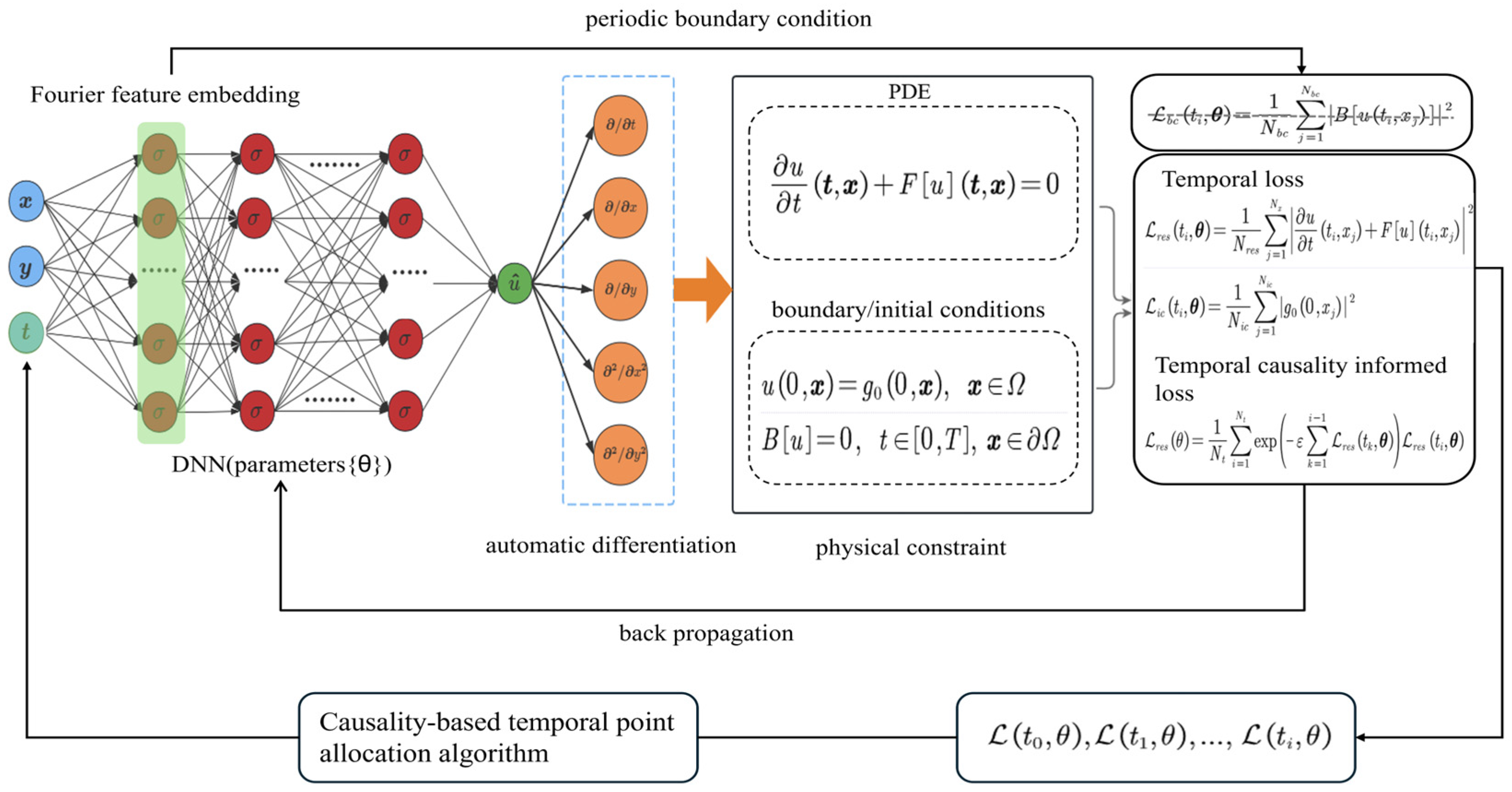
where ${\mathcal{L}}_{pde}$, ${\mathcal{L}}_{\mathit{b}c}$, and ${\mathcal{L}}_{ic}$ represent the losses from the PDE residual, boundary conditions, and initial conditions, respectively. $w_f$, $w_i$, and $w_b$ are their corresponding weights. Figure 1 gives a schematic of the Causal PINN framework for time-dependent problems with periodic boundary conditions in space, which are the main focus of this work.

2.2. Causal PINN

The Causal PINN proposed in [43] is briefly replicated here. Like [43], we mainly focus on problems with the periodic boundary condition $u\left(t,\mathit{x}\right)=u\left(t,\mathit{x}+L\right)$, with wavelength $L$ in a one-dimensional setting. To enforce the periodic boundary condition rigorously, we adopt a hard constraint approach based on Fourier feature embedding. Specifically, we embed the input spatial coordinates into a truncated Fourier series as follows:

$$v\left(\mathit{x}\right)=\left[\begin{array}{c}1,\cos \left(w\mathit{x}\right),\sin \left(w\mathit{x}\right),\cos \left(2w\mathit{x}\right),\sin \left(2w\mathit{x}\right),\dots ,\end{array}\cos \left(mw\mathit{x}\right),\sin \left(mw\mathit{x}\right)\right]$$

(9)

where $w=2\pi /L$, and $m$ is the number of Fourier modes, set to 10 in this work. For any neural network representation using this encoding, it can be shown that the output strictly satisfies the periodic constraint [54]. As a result, the loss function is simplified into two components:

$$\mathcal{L}\left(\mathit{\theta }\right)={\lambda }_{ic}{\mathcal{L}}_{ic}\left(\mathit{\theta }\right)+{\lambda }_{res}{\mathcal{L}}_{res}\left(\mathit{\theta }\right).$$

(10)

For a given set of spatial sampling points ${\left\{{\mathit{x}}_i\right\}}_{i=1}^{N_{\mathit{x}}}$, we define the temporal residual loss ${\mathcal{L}}_{res}\left(t_i,\mathit{\theta }\right)$ as

$${\mathcal{L}}_{res}\left(t_i,\mathit{\theta }\right)={\displaystyle \frac{1}{N_{\mathit{x}}}}{\displaystyle \sum _{j=1}^{N_{\mathit{x}}}{\left|\frac{\partial \widehat{u}}{\partial t}\left(t_i,{\mathit{x}}_j\right)+F\left[\widehat{u}\right]\left(t_i,{\mathit{x}}_j\right)\right|}^2}.$$

(11)

The total residual loss over the entire time domain is given by

$${\mathcal{L}}_{res}\left(\mathit{\theta }\right)={\displaystyle \frac{1}{N_t}}{\displaystyle \sum _{i=1}^{N_t}{w}_i{\mathcal{L}}_{res}}\left(t_i,\mathit{\theta }\right).$$

(12)

where $w_i$ is the temporal weight for $t_i$ and calculated from the residuals in previous times $\left(t_0,t_1,\dots ,t_{i-1}\right)$ as

$$w_i=\exp \left(-\epsilon {\displaystyle \sum _{k=1}^{i-1}{\mathcal{L}}_{res}\left(t_k,\mathit{\theta }\right)}\right).$$

(13)

Then, the weighted residual loss can be written as

$${\mathcal{L}}_{res}\left(\mathit{\theta }\right)={\displaystyle \frac{1}{N_t}}{\displaystyle \sum _{i=1}^{N_t}\exp \left(-\epsilon {\displaystyle \sum _{k=1}^{i-1}{\mathcal{L}}_{res}\left(t_k,\mathit{\theta }\right)}\right){\mathcal{L}}_{res}}\left(t_i,\mathit{\theta }\right).$$

(14)

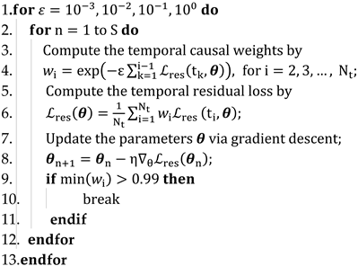
Here, $\epsilon$ is a hyperparameter that controls the steepness of the temporal weight decay. In this work, $\epsilon$ is empirically set to $[{10}^{-3},{10}^{-2},{10}^{-1},{10}^0]$. When $w_i$ is very small, it indicates that the residuals in $t\in \left[1,\dots ,i-1\right]$ have not effectively converged. When the residuals in $t\in \left[1,\dots ,i-1\right]$ are well-converged, $w_i$ will be sufficiently large. In the implementation, the stop criterion is set as $w_i>0.99$. The basic algorithm of the Causal PINN is given below (Algorithm 1).

Algorithm 1. PINNs with the temporal causality

2.2.1. Time Marching

The concept of time marching, although mentioned in Causal PINN, has not been thoroughly analyzed in terms of its impact on the results [43]. Wight and Zhao [48] first implemented this strategy by dividing the temporal domain into successive time segments and sequentially training the network within each segment [55].

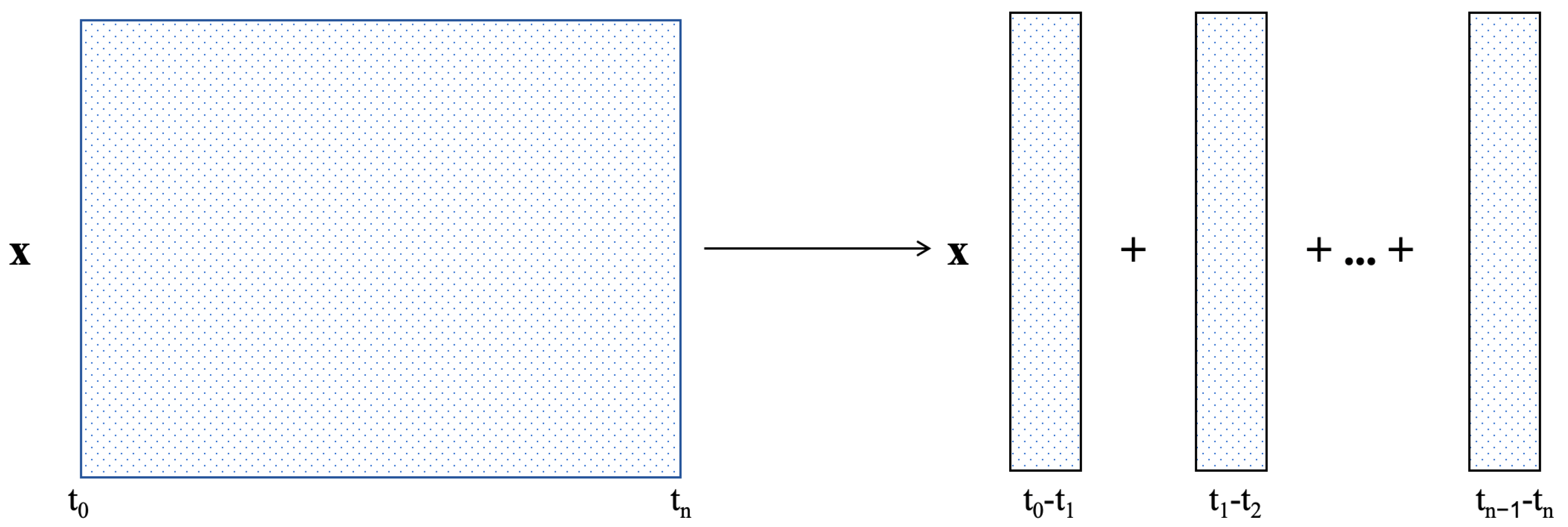
Figure 2 illustrate the time-marching framework. To make full use of temporal information across the entire domain, the time interval $\left[t_0,t_n\right]$ is partitioned as follows:

$$T_0:\left[t_0,t_1\right],T_1:\left[t_1,t_2\right],\dots ,T_{n-1}:\left[t_{n-1},t_n\right]$$

where $T_k,k=0,\dots ,n-1$ denotes the $k$-th time subinterval. In the first interval $\left[t_0,t_1\right]$, training is conducted using the given initial condition. For each subsequent subinterval $\left[t_i,t_{i+1}\right]$, the prediction at the final time point of the previous segment serves as the initial condition for the current segment. A dedicated neural network is constructed within each temporal subinterval. The time and space coordinates within that subdomain are used as inputs for training. This decomposition avoids the shortcomings of global training across the entire temporal domain. Global training in a single domain may lead to the inadequate utilization of local temporal features and result in prediction error and dynamic distortion [48]. The training with time marching progresses sequentially through time: each temporal subdomain is trained one after another until the entire domain is covered. This segmented and progressive time-marching strategy enables full exploitation of local temporal features within each small interval. It also ensures continuity and physical consistency across intervals. As a result, the overall accuracy and stability in solving time-evolution PDEs are significantly improved.

2.2.2. Causality-Based Temporal Point Allocation Algorithm

One unique feature of the present work is the adoption of the causality-based temporal point allocation algorithm. It is an adaptive sampling strategy grounded in the principle of temporal causality. It aims to dynamically adjust the distribution of temporal sampling points to enhance the performance of Causal PINN in solving time-dependent problems.

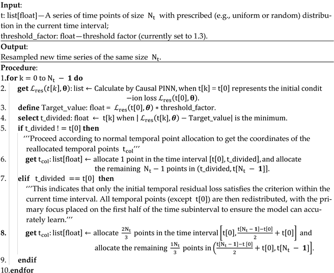
This algorithm uses temporal residual loss to identify regions with large errors. It prioritizes the sampling in these areas to guide the network to learn challenging dynamics better. This idea bears certain similarity to the TCAS-PINN [44], but the actual implementation is different (as seen below, Algorithm 2). Through iterative optimization, this strategy drives the network to incrementally reduce residuals across the time domain, ultimately improving prediction accuracy and convergence speed.

Algorithm 2. Causality-based temporal point allocation algorithm

The algorithm for a given time subinterval proceeds in the following steps:

1.

Initial temporal point allocation

The initial distribution of time points (with the total number being ${\mathrm{N}}_{\mathrm{t}}$) in a given time subinterval can be uniform or non-uniform depending on the characteristics of the problem.

2.

Error evaluation

At each time point, the current PDE residual is computed and compared against a preset threshold, which is an empirical parameter that defines whether the error at a given time point is acceptable. Here, the threshold is set to 130% of the initial temporal residual at the starting point of the current time subinterval (see Figure 3). The setting of this threshold is partly based on the observation that the loss at different time points usually increases with time, and one may relax the criterion for “well-trained” (in a sense relative to the starting point) time points slightly, say, by 30%. The effect of the threshold value will be briefly investigated in Section 3.4.

3.

Dynamic adjustment

The basic idea is to increase the local sampling density where the residual exceeds the threshold and to decrease the sampling density where the residual is below the threshold. Specifically, the point where the local residual is the closest to the threshold is searched first. For convenience, it is labeled as the separation point. If this point is simply the starting point of the current subinterval, two thirds of the ${\mathrm{N}}_{\mathrm{t}}$ points are distributed in the first half of the current subinterval and the other one third are put in the second half. Otherwise, only one point is put between the starting point and the separation point and all other points are distributed after the separation point.

4.

Iterative update

Based on the adjusted time point distribution, the Causal PINN is retrained. This procedure is repeated until the residuals at all time points fall below the threshold.

To better explain the algorithm, we present four typical temporal point distributions at different stages in Figure 4 (for one of the cases studied below). After initializing the neural network, the initial randomly generated sampling points are shown in Figure 4a. Note that the horizontal axis is for time and the vertical axis is for space. During the stage from (a) to (b), as the number of iterations increases, the separation point (t_divided) in the algorithm is some intermediate point in time and it is away from the starting point. Under such conditions, the algorithm causes the temporal sampling points to be progressively redistributed toward later times. After a certain number of iterations, with changes in temporal points and updates to the neural network parameters, the residuals at all time points (except the starting point) eventually fail to meet the preset criterion to determine t_divided. Then, the separation point moves back to the starting point. This triggers the elif condition in the pseudo-code and the time points are redistributed again, with 2/3 of the points in the first half and the remaining 1/3 in the second half of the subinterval. This process is represented by Figure 4b,c. It should be noted that 2/3 and 1/3 in the code block are empirically determined parameters, and the effectiveness of this setting is verified through numerical experiments. The choice of this ratio for the redistribution of time points is partly motivated by the causality principle that the earlier portion of a time interval should be approximated reasonably well by the PINNs first and, therefore, should require more attention. Some discussions on this ratio will be given later in Section 3.4. The process from Figure 4c,d is similar to that from Figure 4a,b.

2.3. The Cahn–Hilliard Equation

The CHE is often used in the study of multiphase flow dynamics. Its fourth-order nature and high nonlinearity pose significant challenges for numerical solution. Accurately solving the CHE using PINNs remains a major challenge. For a system described by the CHE, the total free energy of the CHE system can be defined as

$$E\left(u\right)={\displaystyle {\int }_{\Omega }\left(\frac{{\epsilon }^2}{2}{\left|\nabla u\right|}^2+F\left(u\right)\right)d\mathit{x}},$$

(15)

where $u\left(\mathit{x},t\right)$ is the phase variable, $\epsilon$ is a positive constant related to the interfacial width, and $F\left(u\right)$ is a nonlinear bulk potential. In this study, we adopt the following Ginzburg–Landau double-well potential [56,57]:

$$F_{db}\left(u\right)={\displaystyle \frac{1}{4}}{\left(u^2-1\right)}^2.$$

(16)

Under this free energy formulation, the CHE can be derived via a gradient flow approach as follows:

$$u_t-{\nabla }^2\left(-\alpha \kappa {\nabla }^{2}u+\kappa f\left(u\right)\right)=0,$$

(17)

where the function $f\left(u\right)$ is the derivative of the double-well potential $f\left(u\right)=F^{\prime }\left(u\right)=u^3-u$, and the two minima of the potential (at $u=\pm 1$) correspond to the two phases of the system. The parameter $\kappa$ denotes the mobility, and $\alpha ={\epsilon }^2$ is related to the interface width.

2.4. Causal PINN Solution of the CHE

With different PDE loss definitions, there are two different frameworks for solving the CHE using PINNs. The first is solving the original equation with the fourth-order derivative directly. The other is introducing the chemical potential to transform the equation into two coupled second-order equations. The PDE loss when it is solved directly is defined as follows:

$${\mathcal{L}}_{\mathrm{res}}(\mathit{\theta })={\displaystyle \frac{1}{N_t}}{\displaystyle \frac{1}{N_{\mathit{x}}}}{\displaystyle \sum _{i=1}^{N_t}{\displaystyle \sum _{j=1}^{N_{\mathit{x}}}{w}_i{\left|\frac{\partial \widehat{u}(t_i,{\mathit{x}}_j)}{\partial t}-\kappa {\nabla }^2(-\alpha {\nabla }^2\widehat{u}(t_i,{\mathit{x}}_j)+f(\widehat{u}(t_i,{\mathit{x}}_j)))\right|}^2}}.$$

(18)

where the temporal weight $w_i$ is calculated using Equation (13). However, the direct solution may face optimization problems due to higher-order derivatives. To simplify the computation of derivatives, the more commonly used method is to introduce an intermediate variable—the chemical potential $\phi$ [56,57]. The original CHE is then decomposed into two lower-order PDEs as

$$u_t=\kappa {\nabla }^2\phi ,$$

(19)

$$\phi =-\alpha {\nabla }^{2}u+f\left(u\right).$$

(20)

We design the output layer of the neural network to have two neurons to predict $\phi$ and $u$, denoted by $\widehat{\phi }$ and $\widehat{u}$. Previously, under the time-marching framework, we divided the entire temporal domain into n subintervals. Here, we implement a residual ratio-adaptive weighting scheme inspired by foundational dynamic loss balancing principles in SciML [58,59,60]. Our approach computes PDE residuals adaptively per subinterval. For each temporal interval containing $N_t$ time points and $N_{\mathit{x}}$ spatial points, the loss is formulated as follows:

$$\begin{array}{l}{\mathcal{L}}_{\mathrm{res}1}(\mathit{\theta })={\displaystyle \frac{1}{N_t}}{\displaystyle \frac{1}{N_{\mathit{x}}}}{\displaystyle \sum _{i=1}^{N_t}{\displaystyle \sum _{j=1}^{N_{\mathit{x}}}{w}_i{\left|\frac{\partial \widehat{u}(t_i,{\mathit{x}}_j)}{\partial t}-\kappa {\nabla }^2\widehat{\phi }(t_i,{\mathit{x}}_j)\right|}^2}},\\ {\mathcal{L}}_{\mathrm{res}2}(\mathit{\theta })={\displaystyle \frac{1}{N_t}}{\displaystyle \frac{1}{N_{\mathit{x}}}}{\displaystyle \sum _{i=1}^{N_t}{\displaystyle \sum _{j=1}^{N_{\mathit{x}}}{w}_i{\left|\widehat{\phi }(t_i,{\mathit{x}}_j)-(-\alpha {\nabla }^2\widehat{u}(t_i,{\mathit{x}}_j)+f(\widehat{u}(t_i,{\mathit{x}}_j)))\right|}^2}}.\end{array}$$

(21)

The ratio between the two terms $ratio=L_{res1}\left(\mathit{\theta }\right)/L_{res2}\left(\mathit{\theta }\right)$ is used to balance their contributions in the temporal residual loss function:

$$\begin{array}{l}{\mathcal{L}}_{res1}\left(t_i,\mathit{\theta }\right)={\displaystyle \frac{1}{N_{\mathit{x}}}}{\displaystyle \sum _{j=1}^{N_{\mathit{x}}}{\left|\frac{\partial \widehat{u}\left(t_i,{\mathit{x}}_j\right)}{\partial t}-\kappa {\nabla }^2\widehat{\phi }\left(t_i,{\mathit{x}}_j\right)\right|}^2},\\ {\mathcal{L}}_{res2}(\mathit{\theta })={\displaystyle \frac{1}{N_{\mathit{x}}}}{\displaystyle {\displaystyle \sum _{j=1}^{N_{\mathit{x}}}{\left|\widehat{\phi }(t_i,{\mathit{x}}_j)-(-\alpha {\nabla }^2\widehat{u}(t_i,{\mathit{x}}_j)+f(\widehat{u}(t_i,{\mathit{x}}_j)))\right|}^2}}.\\ {\mathcal{L}}_{res}(\mathit{\theta })={\mathcal{L}}_{res1}(\mathit{\theta })+\mathit{ratio}\times {\mathcal{L}}_{res2}(\mathit{\theta })\end{array}$$

(22)

Through this adaptive weighting mechanism, the magnitudes of both temporal residual losses are kept at the same scale, ensuring the stability of the Causal PINN during training.

$${\mathcal{L}}_{res}\left(t_i,\mathit{\theta }\right)={\mathcal{L}}_{res1}\left(t_i,\mathit{\theta }\right)+ratio\times {\mathcal{L}}_{res2}\left(t_i,\mathit{\theta }\right)$$

(23)

Previous works used fixed weights, with the temporal residual loss given by the following [48,49]:

$${\mathcal{L}}_{res}\left(t_i,\mathit{\theta }\right)={\lambda }_{res1}{\mathcal{L}}_{res1}\left(t_i,\mathit{\theta }\right)+{\lambda }_{res2}{\mathcal{L}}_{res2}\left(t_i,\mathit{\theta }\right)$$

(24)

where ${\lambda }_{res1}$ and ${\lambda }_{res2}$ are two constants.

Two forms of the temporal residual loss expression are now established: one employing fixed weights (24) and another utilizing adaptive weights (23). The difference between them lies in the distinct methods used to control the magnitudes of the residuals for the two sub-equations upon the introduction of the chemical potential. The comparisons between them will be presented subsequently.

3. Results and Discussion

In this section, we first discuss the influence of several factors on the predictive accuracy of the neural network. Then, we present the results of our improved method and validate its efficacy using two distinct CHEs. All computations were executed on an NVIDIA GeForce RTX 4090 graphics processing unit (GPU) (Nvidia, Santa Clara, CA, USA). The software package used for all the computations was Jax 0.4.35 [61]. The reference solutions, against which the prediction accuracy was evaluated, were generated using the Chebfun package V 5.7.0 [62]. The neural network hyperparameters are detailed in Appendix A.

3.1. Quantities of Interest for Result Assessment

The Cahn–Hilliard equation possesses several fundamental physical properties [50], including

(a)

Mass conservation

$${\displaystyle {\int }_{\Omega }u\left(\mathit{x},t\right)d\mathit{x}}={\displaystyle {\int }_{\Omega }u\left(\mathit{x},0\right)d\mathit{x}},\forall t>0.$$

(25)

(b)

Energy dissipation

$$E\left(u\left(t\right)\right)\le E\left(u\left(s\right)\right),\forall t>s.$$

(26)

To evaluate the reliability of the model predictions, we define the relative $l^2$-norm error between the neural network output and the reference solution as described below.

To perform the error analysis at a specific time point, we use the following equation to calculate the error:

$${ϵ}_{error}={\displaystyle \frac{{\left[{\displaystyle {\sum }_{j=1}^N{\left(\widehat{u}\left(t,{\mathit{x}}_j\right)-u\left(t,{\mathit{x}}_j\right)\right)}^2}\right]}^{1/2}}{{\left[{\displaystyle {\sum }_{j=1}^N{\left(u\left(t,{\mathit{x}}_j\right)\right)}^2}\right]}^{1/2}}}.$$

(27)

Similarly, the error over the entire spatiotemporal domain can be found by using the following equation:

$${ϵ}_{error}={\displaystyle \frac{{\left[{\displaystyle {\sum }_{i=1}^N{\displaystyle {\sum }_{j=1}^N{\left(\widehat{u}\left(t_i,{\mathit{x}}_j\right)-u\left(t_i,{\mathit{x}}_j\right)\right)}^2}}\right]}^{1/2}}{{\left[{\displaystyle {\sum }_{i=1}^N{\displaystyle {\sum }_{j=1}^N{\left(u\left(t_i,{\mathit{x}}_j\right)\right)}^2}}\right]}^{1/2}}}.$$

(28)

In the first test case, we consider the following setting [49]:

$$\begin{array}{l}u\left(\mathit{x},0\right)=\cos \left(\pi \mathit{x}\right)-\exp \left(-4{\left(\pi \mathit{x}\right)}^2\right),\\ \alpha =0.02,\kappa =1\end{array}$$

(29)

This initial condition describes a perturbation superimposed on a cosine function, where the exponential term introduces a localized sharp variation. The relatively large value of $\kappa$ leads to strong interfacial effects, and the value of $\alpha$ affects the interface thickness.

In the second test case, we consider a different setting [48]:

$$\begin{array}{l}u\left(\mathit{x},0\right)=-\cos \left(2\pi \mathit{x}\right),\\ \alpha ={10}^{-4},\kappa =0.01\end{array}$$

(30)

This initial setup corresponds to a periodic phase distribution. It has a relatively small interface energy coefficient $\kappa$ and a very sharp interface controlled by a small $\alpha$. This case challenges the model’s capacity to resolve fine-scale structures and steep gradients in the phase field.

3.2. Discussion of Parameters and Settings Affecting Solution Performance

Using Case 1 as an example, we first compare different settings in several aspects: (1) Causal PINN with and without time marching; (2) a direct solution versus a solution with intermediate variables; and (3) the use of fixed versus adaptive weights for the two PDE loss terms for the chemical potential formulation. Subsequently, we select an optimal scheme based on these comparisons. By integrating this scheme with our proposed causality-based temporal point allocation algorithm, we introduce an improved method termed APM-PINN.

3.2.1. Causal PINN vs. Causal PINN with Time Marching

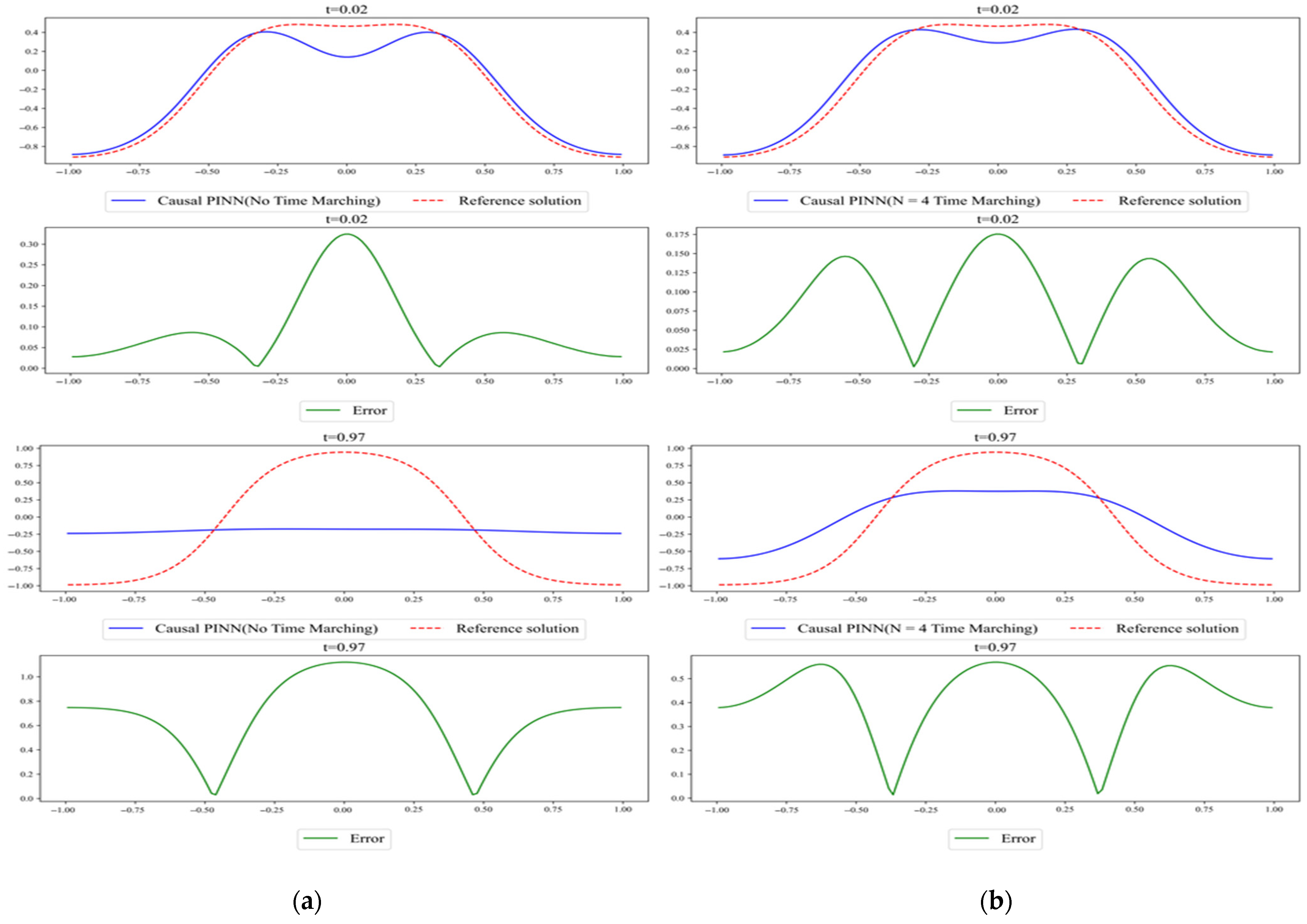
To demonstrate the necessity of incorporating a time-marching strategy, we first solve the CHE in Case 1 using the standard Causal PINN. We compare the performance of Causal PINN under two configurations: one without time marching (i.e., N = 1), and another with a four-step time-marching scheme (i.e., N = 4), as shown in the figures below.

Figure 5 shows that the N = 4 time-marching improves solution accuracy as compared with that with no time-marching (N = 1). This confirms the effectiveness of time marching for high-order dynamical systems. Figure 6 further confirms that the predicted mass and energy evolution curves with the time-marching scheme align more closely with the reference values. This indicates that the solution by time marching has improved conservation property and physical fidelity.

Table 1. Comparison of the relative error ${ϵ}_{error}$ between Causal PINN with and without time marching.

Time	$\mathbf{Relative} {\mathit{L}}^2$ Error (N = 1)	$\mathbf{Relative} {\mathit{L}}^2$ Error (N = 4)
0.02	0.2260	0.1765
0.12	0.6680	0.4558
0.37	0.8882	0.5367
0.5	0.9213	0.5388
0.97	0.9583	0.5633

shows the relative errors of the two methods with respect to the reference solution at a few specific time points. The standard Causal PINN (N = 1) with the entire time domain sampled faces challenges in global temporal optimization. In contrast, the time-marching strategy (N = 4) divides the time domain into four subintervals, performs localized training and passes the solution forward through intermediate initial conditions. This segmented optimization avoids issues such as gradient vanishing or explosion and enables more effective capture of local temporal features [63]. It results in significantly reduced relative error—for instance, a 39.5% error reduction at t = 0.97. In long-time simulations, standard Causal PINN suffers from accumulated prediction errors, with residuals exceeding 0.9 beyond t = 0.5. That indicates a substantial deviation from the ground truth.

In conclusion, the time-marching strategy improves the solution capability of Causal PINN for high-order nonlinear PDEs by enabling localized optimization and error isolation across temporal intervals. It is thus essential for long time-evolution problems. All subsequent numerical experiments in this study adopt the time-marching framework.

3.2.2. Direct Solution vs. Chemical Potential Reformulation

In this section, we focus on whether introducing intermediate variables can improve the predictive performance of the model. All experiments were conducted under the time-marching framework described in Section 2.2.1, where the entire temporal domain $\left[t_0,t_n\right]$ is divided into four subintervals $\left[t_0,t_1\right],\left[t_1,t_2\right],\left[t_2,t_3\right],\left[t_3,t_4\right]$ of the same size. Each subinterval is trained with an independent Causal PINN model.

Recalling Equations (18), (22) and (24), the primary difference between direct solution and chemical potential reformulation lies in the distinct PDE temporal loss term within the loss function.

$$\mathrm{direct}\mathrm{solution}:{\mathcal{L}}_{\mathrm{res}}\left(t_{\mathrm{i}},\mathit{\theta }\right)={\displaystyle \frac{1}{N_x}}{\displaystyle \sum _{j=1}^{N_x}{\left|\frac{\partial \hat{u}\left(t_i,x_j\right)}{\partial t}-{\nabla }^2\left(-\alpha \kappa {\nabla }^2 \hat{u}\left(t_i,x_j\right)+\kappa f\left( \hat{u}\left(t_i,x_j\right)\right)\right)\right|}^2}$$

(31)

$$\begin{array}{l}\hspace{1em}\hspace{1em}\hspace{1em}\hspace{1em}\hspace{1em}\hspace{1em}\hspace{1em}\hspace{1em}\hspace{1em}\hspace{1em}\hspace{1em}\hspace{1em}\hspace{1em}\hspace{1em}{\mathcal{L}}_{res1}\left(t_i,\mathit{\theta }\right)={\displaystyle \frac{1}{N_{\mathit{x}}}}{\displaystyle \sum _{j=1}^{N_{\mathit{x}}}{\left|\frac{\partial \widehat{u}\left(t_i,{\mathit{x}}_j\right)}{\partial t}-\kappa {\nabla }^2\widehat{\phi }\left(t_i,{\mathit{x}}_j\right)\right|}^2},\\ \mathrm{chemical} \mathrm{potemtial} \mathrm{reformulation}: {\mathcal{L}}_{res2}(\mathit{\theta })={\displaystyle \frac{1}{N_{\mathit{x}}}}{\displaystyle {\displaystyle \sum _{j=1}^{N_{\mathit{x}}}{\left|\widehat{\phi }(t_i,{\mathit{x}}_j)-(-\alpha {\nabla }^2\widehat{u}(t_i,{\mathit{x}}_j)+f(\widehat{u}(t_i,{\mathit{x}}_j)))\right|}^2}}.\\ \hspace{1em}\hspace{1em}\hspace{1em}\hspace{1em}\hspace{1em}\hspace{1em}\hspace{1em}\hspace{1em}\hspace{1em}\hspace{1em}\hspace{1em}\hspace{1em}\hspace{1em}\hspace{1em}{\mathcal{L}}_{res}\left(t_i,\mathit{\theta }\right)={\lambda }_{res1}{\mathcal{L}}_{res1}\left(t_i,\mathit{\theta }\right)+{\lambda }_{res2}{\mathcal{L}}_{res2}\left(t_i,\mathit{\theta }\right)\end{array}$$

(32)

For the chemical potential reformulation, we apply an appropriate weighting scheme to balance the temporal loss terms with ${\lambda }_{res1}=100$ and ${\lambda }_{res2}=1$. For both algorithms, when calculating the total loss, the weight for the initial condition loss ${\lambda }_{ic}$ is set to 100.

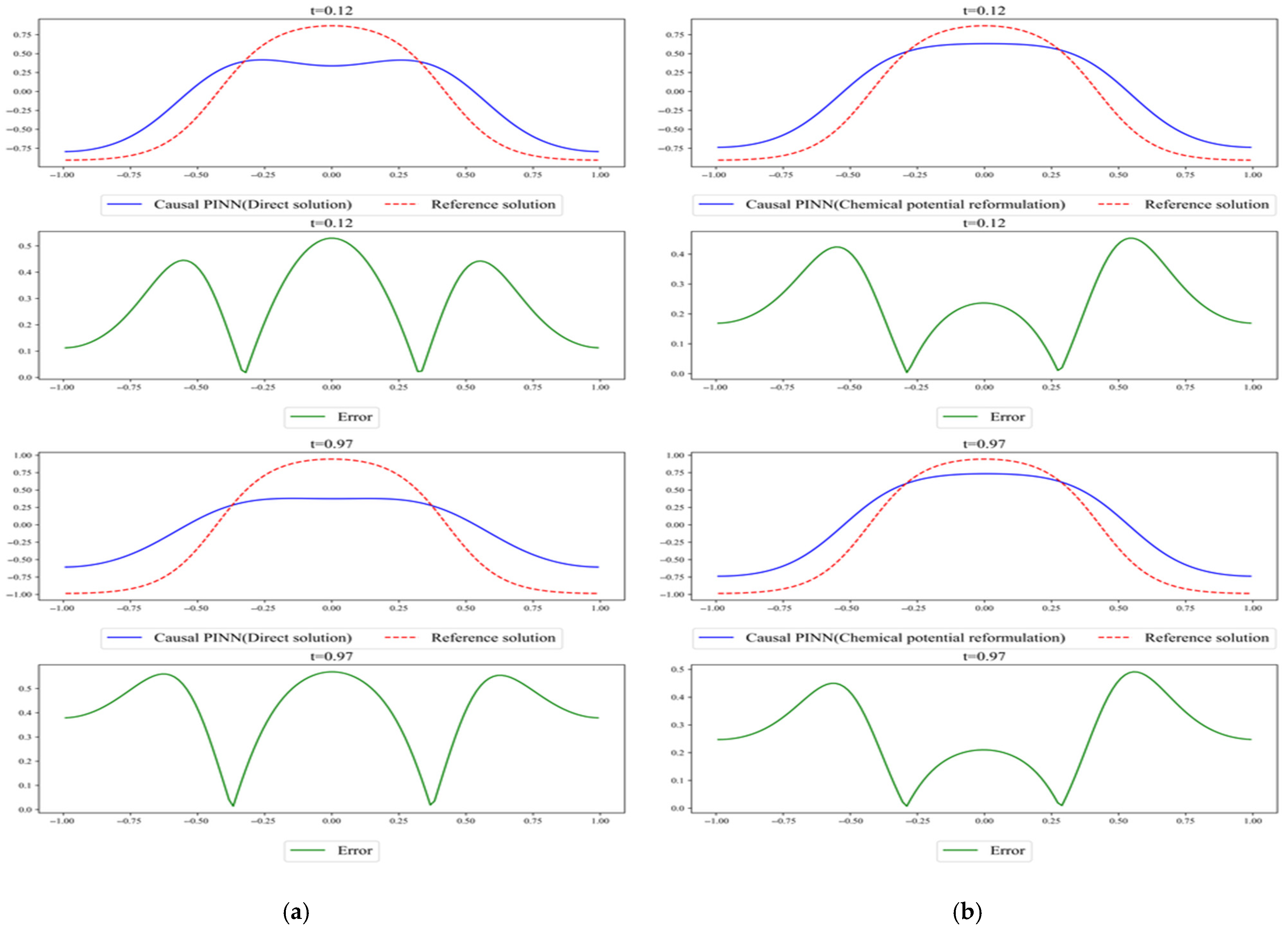
Figure 7 shows the comparison of the results predicted via (a) the direct solution and (b) chemical potential reformulation. Figure 8 shows the comparison of the evolutions of mass and energy. The results show that, compared to the reference solution, the outcomes from both methods still exhibit significant errors. However, the introduction of intermediate variables and the assignment of appropriate weights can nevertheless reduce the errors.

From

Table 2. Comparison of the relative error ${ϵ}_{error}$ between direct solution and chemical potential reformulation (both using Causal PINN with four time-marching steps).

Time	$\mathbf{Relative} {\mathit{L}}^2$ Error (Direct)	$\mathbf{Relative} {\mathit{L}}^2$ Error (Chemical Potential)
0.02	0.1765	0.1437
0.12	0.4558	0.3795
0.37	0.5367	0.4084
0.5	0.5388	0.4000
0.97	0.5633	0.3828

, it is seen that the prediction error is reduced by 12.8% at t = 0.37 when using the chemical potential formulation. This confirms that the approach not only simplifies the computational process but also improves predictive accuracy. However, despite its effectiveness, the chemical potential method still requires manual tuning of the loss weights. Improper settings of the weights may cause imbalance between the temporal residual terms ${\mathcal{L}}_{res1}\left(t_i,\mathit{\theta }\right)$ and ${\mathcal{L}}_{res2}\left(t_i,\mathit{\theta }\right)$ and affect training stability. To address this issue, we further introduce an adaptive loss weighting mechanism as detailed in Section 2.4.

3.2.3. Static vs. Adaptive Loss Weighting

We revisit two forms of temporal loss function introduced in Section 2.4 (cf. Equations (23) and (24)):

$$\begin{array}{l}{\mathcal{L}}_{res}\left(t_i,\mathit{\theta }\right)={\mathcal{L}}_{res1}\left(t_i,\mathit{\theta }\right)+ratio\ast {\mathcal{L}}_{res2}\left(t_i,\mathit{\theta }\right)\\ {\mathcal{L}}_{res}\left(t_i,\mathit{\theta }\right)={\lambda }_{res1}{\mathcal{L}}_{res1}\left(t_i,\mathit{\theta }\right)+{\lambda }_{res2}{\mathcal{L}}_{res2}\left(t_i,\mathit{\theta }\right)\end{array}$$

For the fixed weights, we apply an appropriate weighting scheme to balance the loss terms with ${\lambda }_{res1}=100$ and ${\lambda }_{res2}=1$. For both approaches to obtaining the total loss, we use the same initial condition loss weight ${\lambda }_{ic}=100$. Next, we compare the performance of the fixed weighting and the adaptive weighting schemes. All experiments are conducted under the time-marching framework, where the entire temporal domain is evenly divided into four subintervals. Each subinterval is trained independently with its own neural network, and the prediction at the end of the previous subinterval is used as the initial condition for the current one, enabling step-by-step temporal propagation.

Fixed weights, though tunable at the beginning, cannot adapt to dynamic residual changes. As a result, one residual component may dominate the optimization process during certain time intervals and ultimately degrade the overall predictive accuracy. In contrast, the adaptive weighting scheme employs a dynamic residual-based weighting strategy. It continuously monitors the magnitude of the residuals corresponding to the equation for the chemical potential and that for the original variable during training. Based on such information, it adjusts their respective weights in time. This enables the model to automatically balance the optimization direction across different stages of training. The adaptive mechanism reduces the dependence on manual hyperparameter tuning and enhances the model’s robustness and generalization capability.

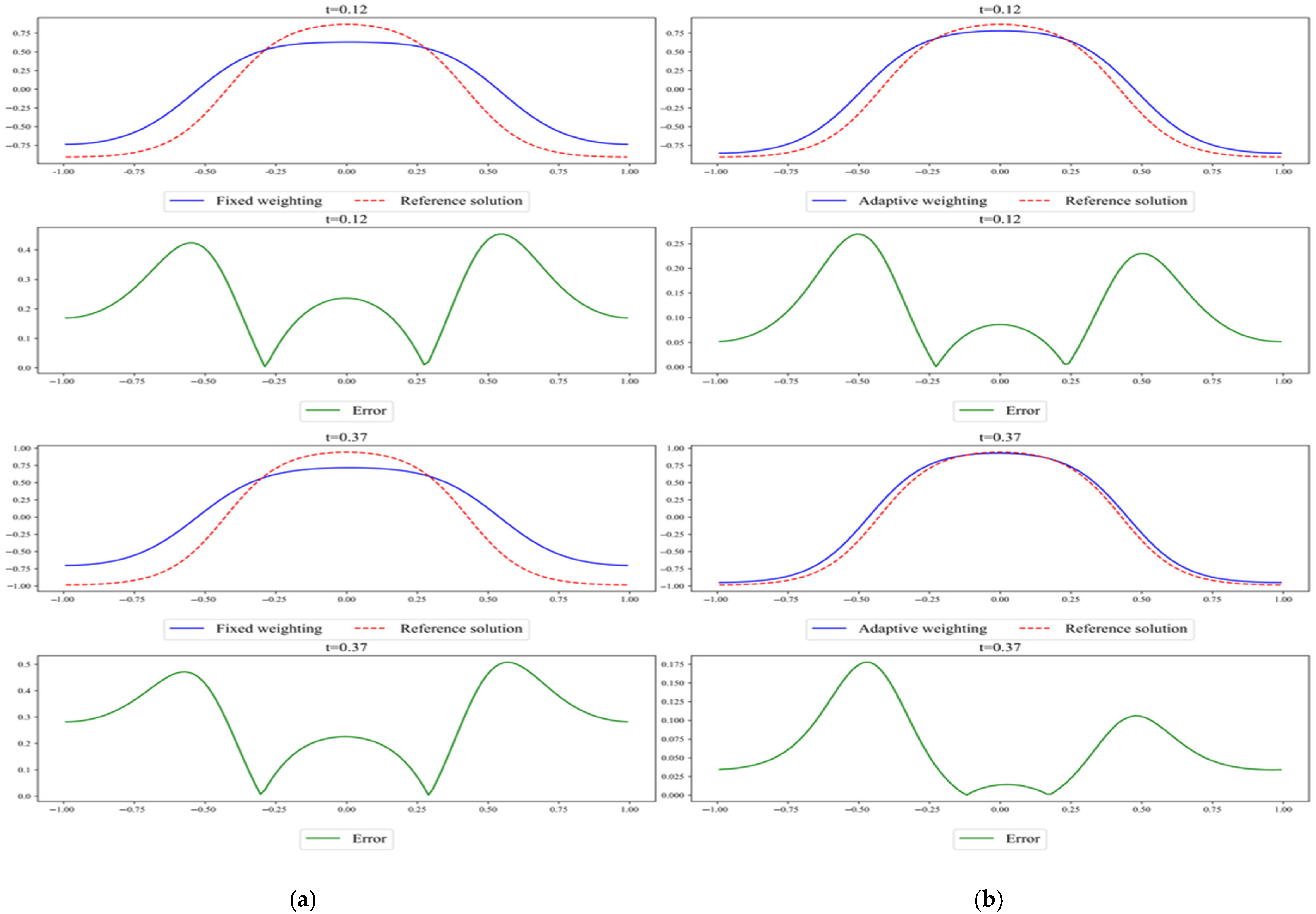
From Figure 9, it is evident that the adaptive weighting method outperforms the fixed weighting strategy at both t = 0.12 and t = 0.37. As found in

Table 3. Comparison of the relative error ${ϵ}_{error}$ between fixed weighting and adaptive weighting (both using Causal PINN with time marching).

Time	$\mathbf{Relative} {\mathit{L}}^2$ Error (Fixed Weighting)	$\mathbf{Relative} {\mathit{L}}^2$ Error (Adaptive Weighting)
0.02	0.1437	0.1020
0.12	0.3795	0.1948
0.37	0.4084	0.1022
0.5	0.4000	0.1037
0.97	0.3828	0.1069

, the relative errors ${ϵ}_{error}$ at t = 0.02, 0.12, 0.37, 0.5, and 0.97 for the adaptive weighting method are 0.1020, 0.1948, 0.1022, 0.1037, and 0.1069, respectively. For the fixed weighting method, they are 0.1437, 0.3795, 0.4084, 0.4000, and 0.3828, respectively. These results clearly demonstrate that the adaptive weighting mechanism offers significant advantages in capturing temporal evolution and maintaining model stability. The improvements are particularly evident during the mid-to-late stages (t = 0.37∼0.97). This indicates that this approach holds strong potential for generalization in long time-evolution problems. From the convergence curves of the loss function in Figure 10, the adaptive strategy demonstrates superior convergence efficiency: it converges 1–2 orders of magnitude better than the fixed weighting method in the later three subintervals.

Within the time-marching framework, the adaptive method also maintains stable performance across consecutive time intervals. In contrast, the fixed weighting scheme exhibits noticeable prediction error in certain intervals. This is because prediction errors at the end of one subinterval can be passed as inaccurate initial conditions to the next, and the error gradually accumulates. This accumulation leads to significant degradation in solution quality over a long time. In contrast, the adaptive weighting method offers a residual-aware, dynamically balanced training mechanism. It effectively suppresses error accumulation through in-time adjustment of the optimization trajectory, particularly in subdomains prone to instability. This mechanism not only improves accuracy but also stabilizes training across subintervals.

3.3. Results Obtained by APM-PINN

In the preceding sections, we systematically analyzed how the time-marching strategy improves the accuracy of Causal PINN, explored the effect of introducing intermediate variables (i.e., the chemical potential $\phi$), and compared the performance of fixed weighting with the adaptive weighting strategy for the solution of the 1-D CHE. Building on these foundations, we further improve the time-marching framework by incorporating the causality-based temporal point allocation algorithm introduced in Section 2.2.2. This enhancement is designed to strengthen the model’s expressiveness at critical time points and improve training efficiency.

By integrating these three key improvements—time marching, causality-based temporal point allocation algorithm, and adaptive loss weighting—we propose a new solution framework: APM-PINN. This method represents an enhanced extension of the classical Causal PINN. It is able to improve both the accuracy and stability in modeling dynamic systems, as seen from the results presented below. For ease of understanding, the flowchart of the complete APM-PINN code is given in the Appendix A.

3.3.1. Case 1

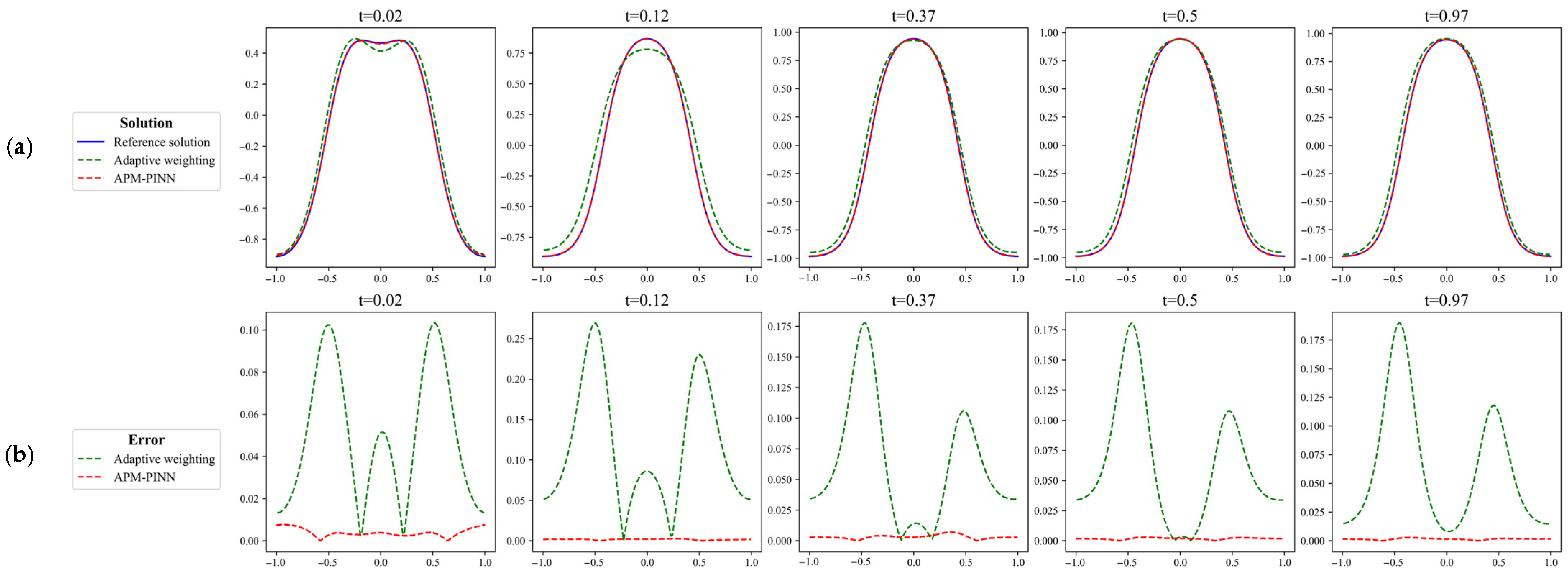
As shown in Figure 11, the introduction of the causality-based temporal point allocation algorithm effectively reduces the loss corresponding to different time intervals. Compared to the adaptive weighting method that does not utilize this algorithm, the relative error is reduced from the order of 10⁻¹ to 10⁻³, while significantly minimizing the range of error fluctuations. Figure 12 and Figure 13 show the good prediction results of the APM-PINN at five selected times and over the entire domain, respectively. Figure 14 shows a comparison of the evolutions of mass and energy. These results indicate that the APM-PINN maintains high solution accuracy throughout the temporal domain. Compared with the traditional Causal PINN, our method enables more effective exploitation of temporal information and significantly reduces the overall error.

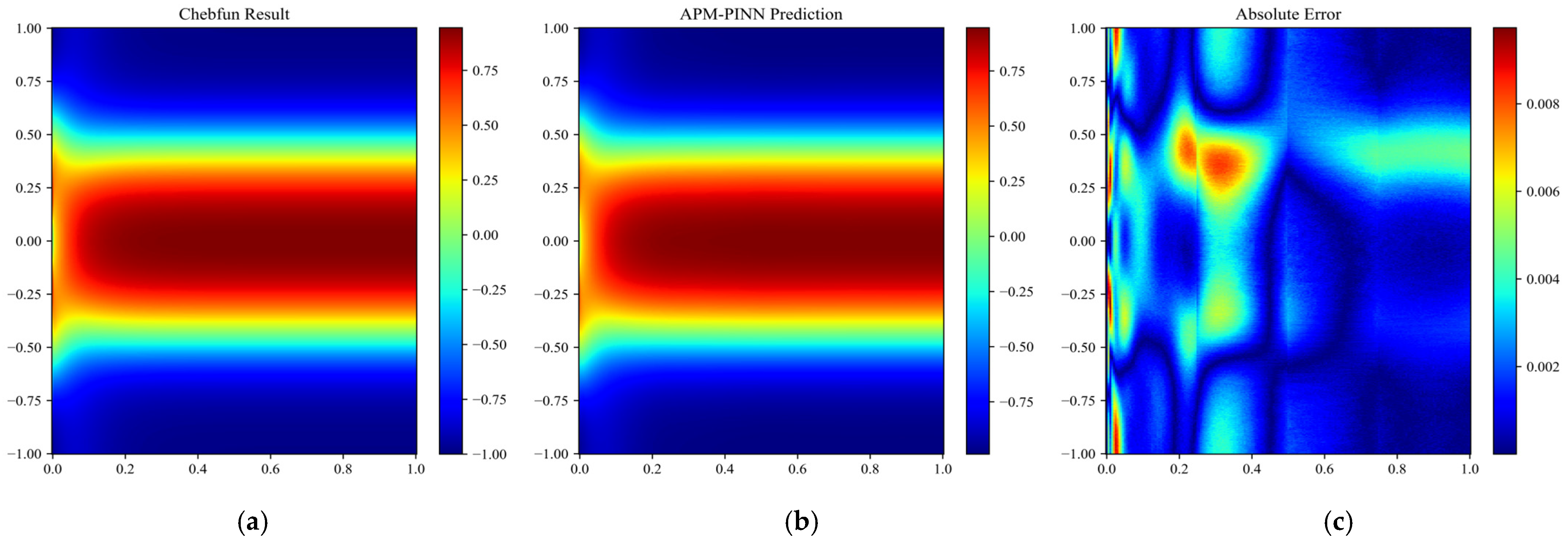
From

Table 4. Relative errors of APM-PINN ${ϵ}_{error}$ for Case 1 at t = 0.02, 0.12, 0.37, 0.5, and 0.97.

Time	$\mathbf{Relative} {\mathit{L}}^2$ Error
0.02	0.007499
0.12	0.002452
0.37	0.004565
0.5	0.002475
0.97	0.002097

, it is obvious that the APM-PINN reduces the relative error to an order of 10⁻³ at all monitoring time points, representing a 1–2-order-of-magnitude improvement over the traditional Causal PINN, which yields errors on the order of 10⁻¹, as shown in Section 3.2.1. More comparisons between different PINN methods are shown in

Table 5. Comparison of overall relative $L^2$ errors for Case 1 using different PINN methods, including the Standard-PINNs, bc-PINN, TCAS-PINN, and APM-PINN, with varying numbers of neurons and training points [44,49]. For APM-PINN, N = 4 time marching was used and the number of points is for one time interval. The results of APM-PINN are obtained from five runs with different network initializations, and the mean value and standard deviation are given.

Method	Number of Neurons	Number of Points	Relative Error
Standard-PINNs	4 × 128	1000	1.025
bc-PINN	4 × 200	20,000	0.03600
TCAS-PINN	4 × 128	1000	0.004568
APM-PINN	4 × 64	16 × 128	0.005005 ± 0.001416

. Note that to ensure reproducibility, five sets of numerical experiments with different network initializations were performed using APM-PINN. It can be seen that the accuracy of APM-PINN is comparable to that of TCAS-PINN and improves at least by an order of magnitude when compared to bc-PINN and Standard-PINN. At t = 0.97, the relative error predicted by APM-PINN is as low as 0.002097, demonstrating the method’s ability to accurately capture the dynamic features of long time-evolution processes. Compared with other methods shown in Table 3.5, our method also demonstrates strong competitiveness in terms of the overall error. With fewer neural network nodes, we achieve very low relative errors. From the mass conservation and energy dissipation curves in Figure 14, we make the following observations: The mass evolution predicted by APM-PINN is very close to the reference result, with a maximum deviation below 4.7%. This confirms that the algorithm reasonably adheres to the conservation property of the CHE. The total energy decreases monotonically with time, consistent with the theoretical dissipation law. At t = 0.37, the relative energy error is only 0.9%, which is substantially better than that of the standard Causal PINN (where the relative error is approximately 54%; see Section 3.2.1). This demonstrates that the improved method prevents physical inconsistency caused by optimization bias. From Figure 15, it can be seen that the losses reach convergence at around 100,000 steps. Compared with the direct solution using the standard Causal PINN (shown in Figure 5), APM-PINN reduces the relative error at t = 0.5 from 0.9213 to 0.002475. This highlights the critical role of localized time-domain training in effectively suppressing error accumulation.

3.3.2. Case 2

In Case 2, we further evaluate the capability of the APM-PINN in solving the CHE for problems with steep gradients. Compared to Case 1, Case 2 involves much steeper changes and more intense dynamic evolution. This poses greater challenges to the model’s stability and accuracy.

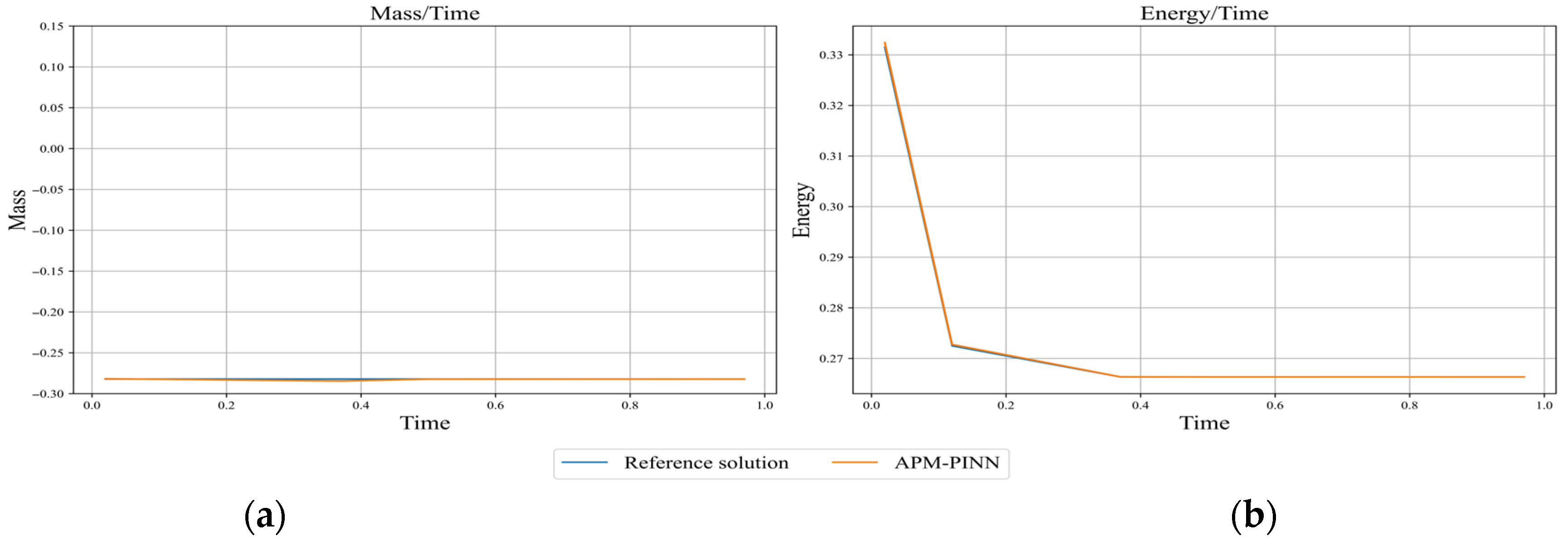
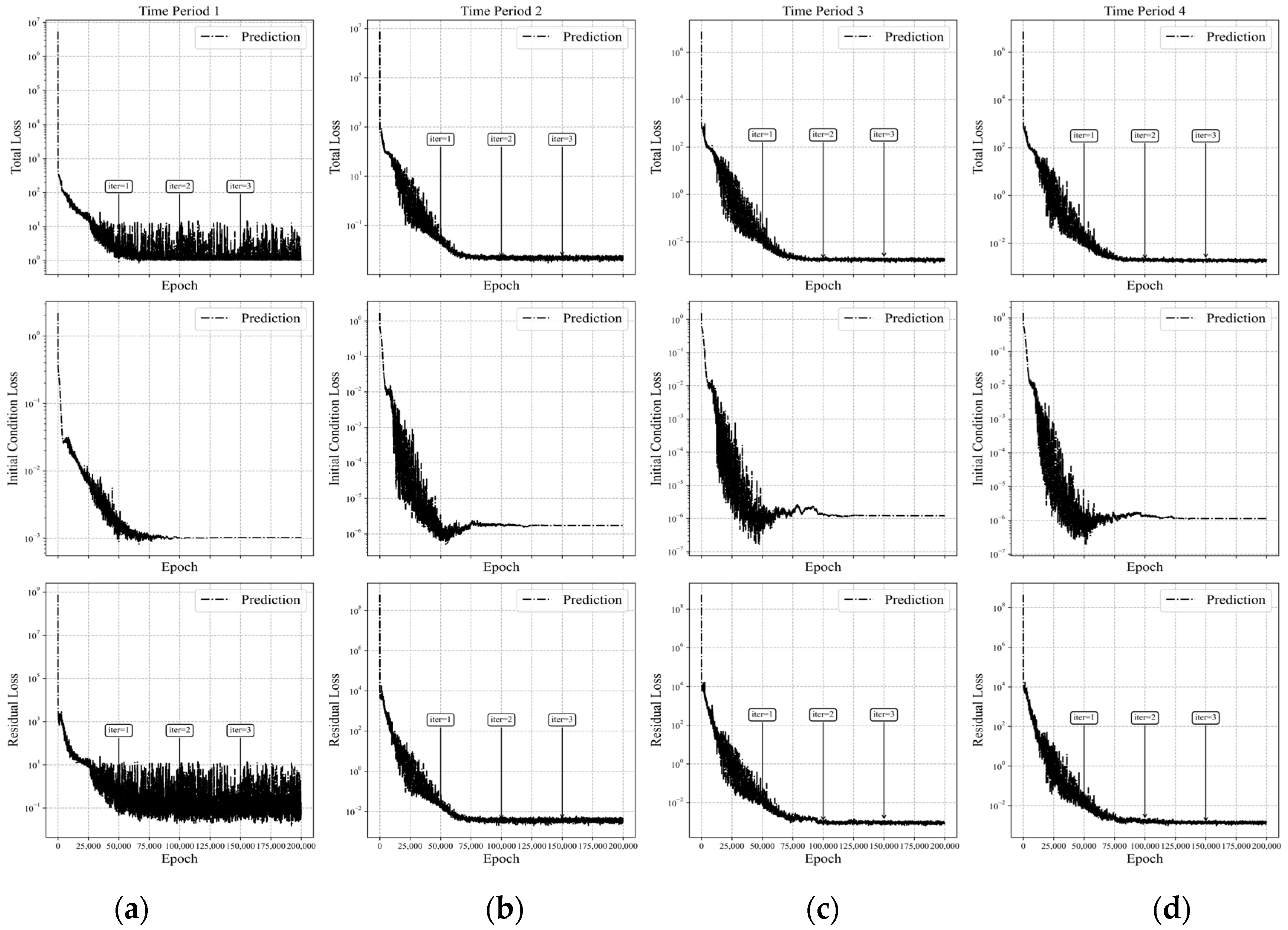
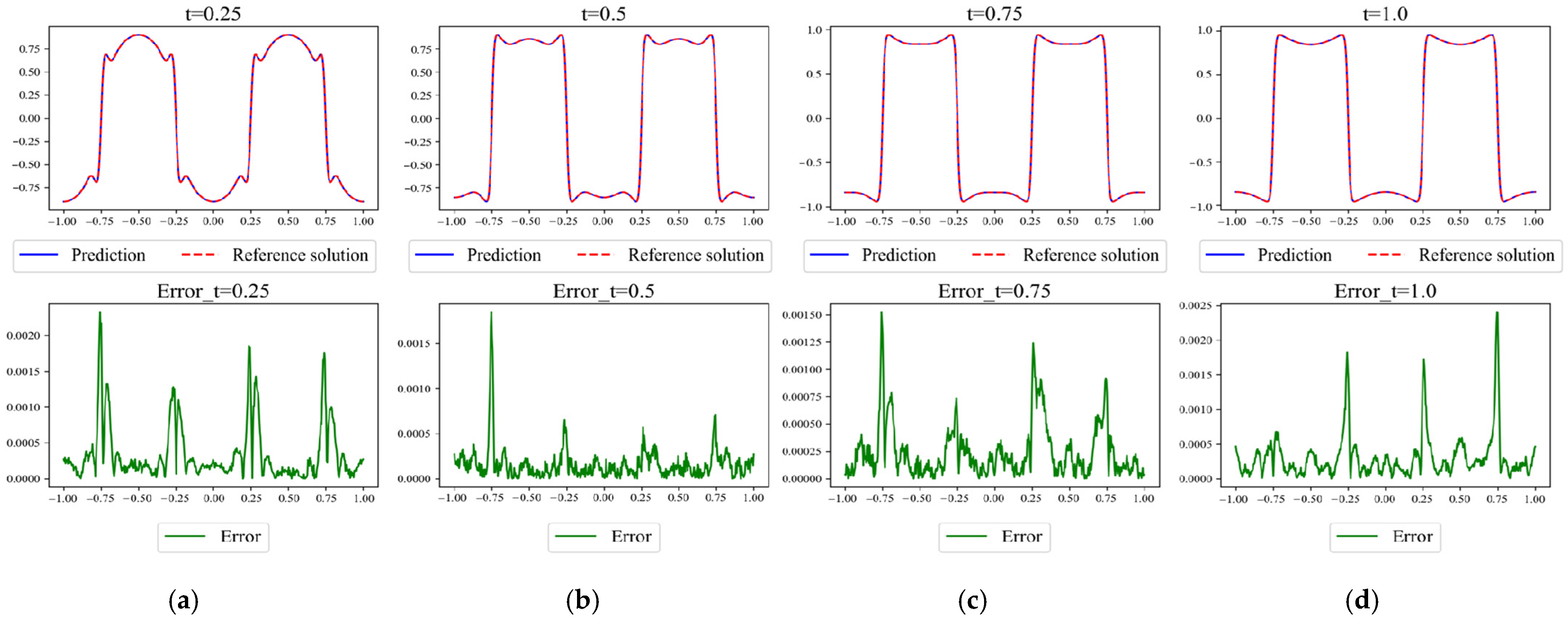
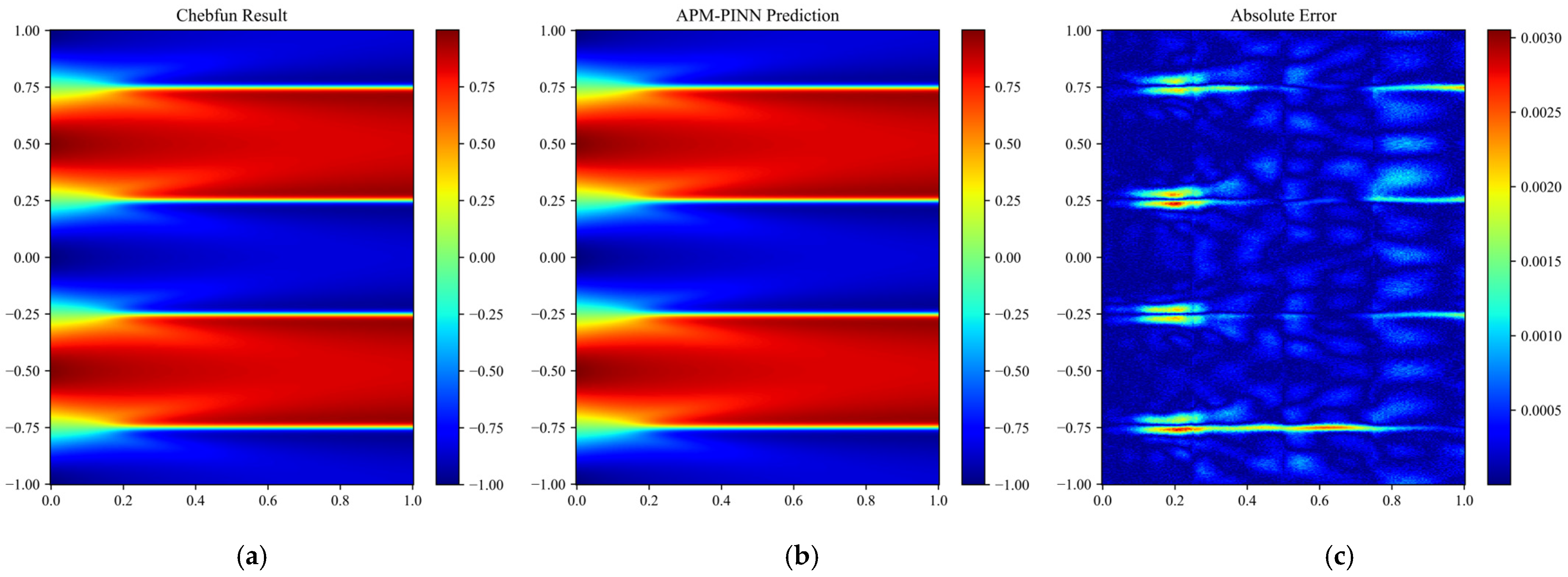
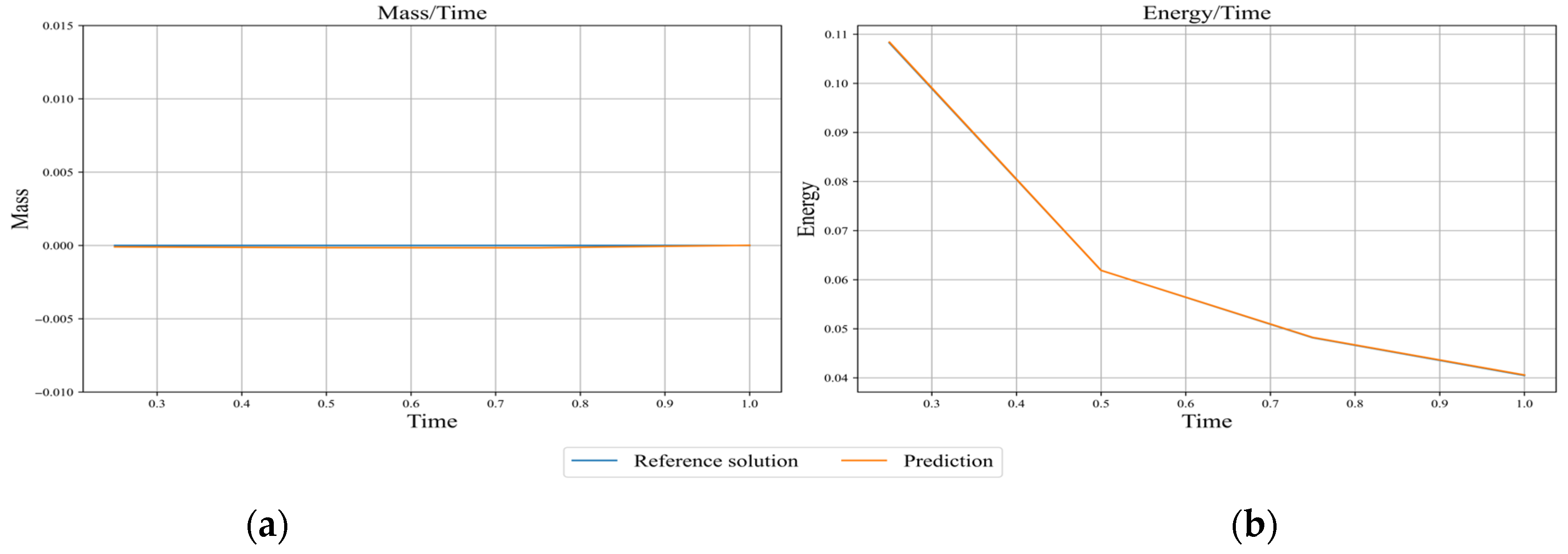
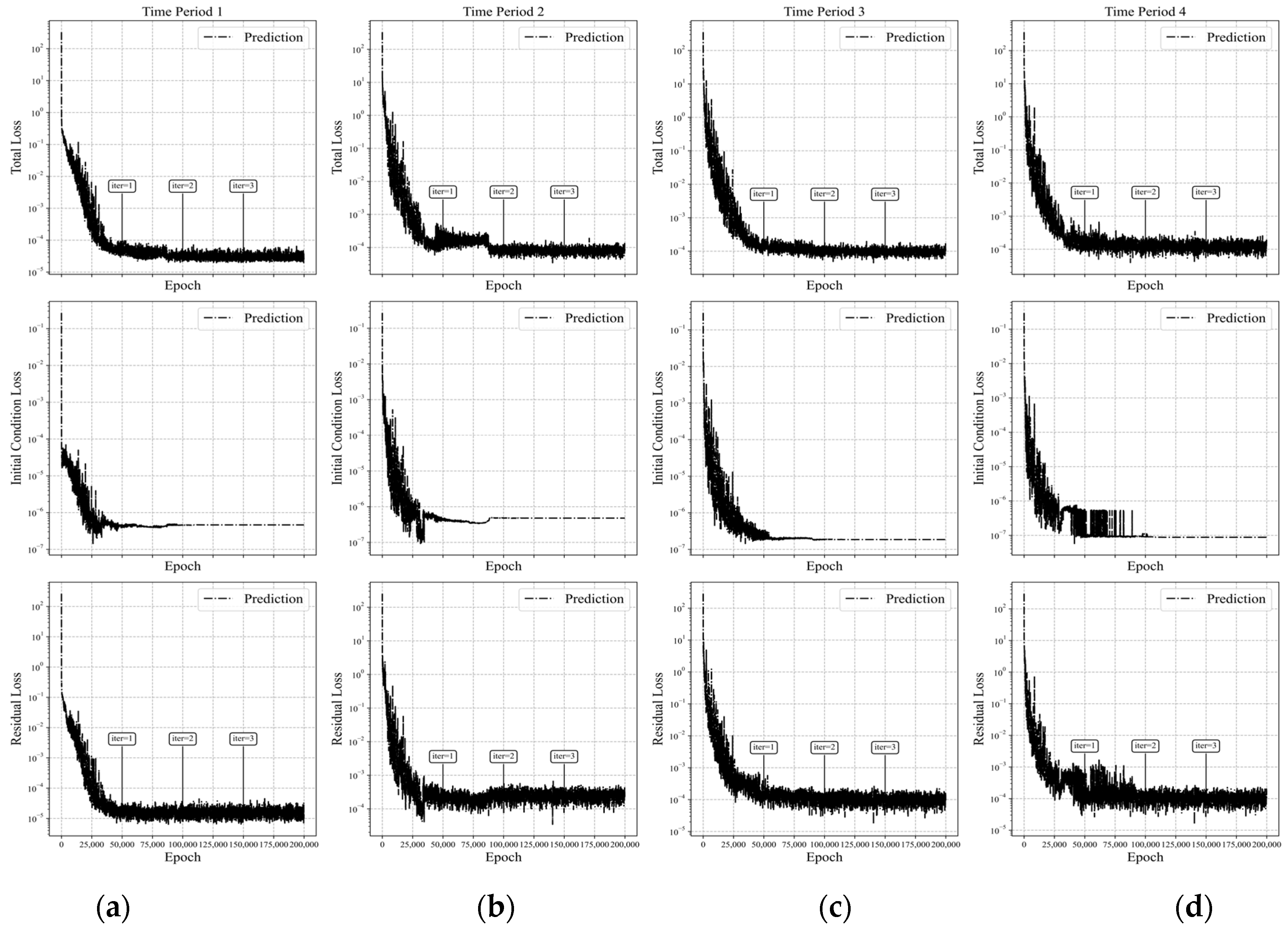
Figure 16 and Figure 17 present the prediction performance of APM-PINN for Case 2 at four selected times and over the entire domain, respectively. The results show that the model accurately captures the key dynamical features of the 1-D CHE solution throughout the entire evolution process. The predicted solutions are close to the reference solutions.

Table 6. Relative errors of APM-PINN ${ϵ}_{error}$ for Case 2 at t = 0.25, 0.50, 0.75, and 1.0.

Time	$\mathbf{Relative} {\mathit{L}}^2$ Error
0.25	0.0006993
0.5	0.0003035
0.75	0.0004053
1.0	0.0005116

shows that the APM-PINN reduces the relative error to an order of 10⁻⁴ at all monitored time points. In addition,

Table 7. Comparison of the overall relative error for Case 2 using different PINN methods, including the improved PINNs in [48] and the present APM-PINN, with different numbers of neurons and training points. For APM-PINN, N = 4 time marching was used and the number of points is for one time interval. Note that “-” means the information is not found in the original paper. The results of APM-PINN are obtained from five runs with different network initializations, and the mean value and standard deviation are given.

Method	Number of Neurons	Number of Points	Relative Error
Improved PINNs	6 × 128	-	0.00951
APM-PINN	4 × 64	16 × 128	0.0005886 ± 0.00008482

compares the relative errors of the improved PINNs in [48] and the present APM-PINN. It is seen that the current method reduces the error by an order of magnitude. These results demonstrate that the proposed method maintains good generalization ability and numerical stability even under more complex conditions. As shown in Figure 18, the model also preserves the physical properties of the CHE in Case 2. The predicted mass evolution is nearly indistinguishable from the reference result, and the energy variation also matches the theoretical trend. These further confirm the model’s superior physical consistency. From the loss convergence curves in Figure 19, it is evident that the improved method also converges rapidly in Case 2. The final loss values are significantly reduced for all subintervals, indicating that the model maintains stable and efficient optimization even under complex conditions with sharp interfaces.

3.4. Sensitivity Analysis of Hyperparameter Robustness

In Section 3.3, we discussed the performance of the neural network after the introduction of the causality-based temporal point allocation algorithm. In this section, we carry out further sensitivity analyses on the numbers of sampling points and time intervals, and two empirical parameters in the causality-based temporal point allocation algorithm. We also make some comparisons with existing methods. Here, we take Case 1 as an example.

Table 8. Comparison of the relative $L^2$ errors of three methods for Case 1, TCAS-PINN, APM-PINN, and Standard-PINN, with varying numbers of neurons and training points [48]. Note that the results presented for TCAS-PINN and Standard-PINN are from [44]. For APM-PINN, N = 4 time marching was used and the number of points is for one time interval.

Method	Number of Neurons	Number of Points	$\mathbf{Relative} {\mathit{L}}^2$ Error
APM-PINN	4 × 64	8 × 128	0.016341
	4 × 64	16 × 128	0.003203
	4 × 64	32 × 128	0.002907
TCAS-PINN	4 × 128	1000	0.004568
	4 × 128	2000	0.004447
	4 × 128	3000	0.004393
Standard-PINN	4 × 128	1000	1.025
	4 × 128	2000	1.031
	4 × 128	3000	1.020

shows the change in the prediction accuracy of the neural network for different numbers of temporal points (8, 16, and 32) used in training for APM-PINN using N = 4 time marching. The number of spatial points is fixed at 128. The results for TCAS-PINN and Standard-PINN are also included for comparison. From this table, it is observed that the number of time points in each time interval affects the accuracy of the results of APM-PINN. The use of too few time points may degrade the accuracy significantly. With a sufficient number of time points, the relative error of our proposed method consistently remains on the order of 10⁻³, demonstrating its effectiveness and reliability. The results highlight that the present APM-PINN has certain advantages in accuracy and robustness for solving complex high-order PDEs compared with existing PINN methods.

Table 9. Comparison of the relative errors of APM-PINN with different numbers of time intervals for Case 1. The neuron number is fixed at 4 × 64 and the number of points per interval is fixed at 16 × 128.

Method	Number of Points	Number of Time Intervals	$\mathbf{Relative} {\mathit{L}}^2$ Error
APM-PINN	16 × 128	4	0.003203
	16 × 128	8	0.005293
	16 × 128	16	0.005490

shows the relative error of APM-PINN using different numbers of time intervals with the number of training points (per interval) fixed at 16 × 128. It is seen that increasing the number of time intervals beyond four does not bring further improvement to the prediction accuracy. On the contrary, the relative error actually increases slightly, but maintains at the order of 10⁻³. These results demonstrate the reliability of APM-PINN to some extent.

Next, we briefly study the effects of two empirical parameters in the causality-based temporal point allocation algorithm, namely, the value of the threshold_factor and the ratio of the number of temporal sampling points in the first and second half of the time interval for the redistribution triggered by the condition “t_divided == t[0]”.

Table 10. Comparison of the relative errors with different values for the threshold_factor in the causality-based temporal point allocation algorithm. N = 4 time marching is used, and the number of points is fixed at 16 × 128. The ratio of the number of temporal sampling points in the first and second half of the time interval for the redistribution (triggered by the condition “t_divided == t[0]”) is fixed at 2/1.

Method	Threshold_Factor	Ratio	Relative Error
APM-PINN	1.1	2/1	0.006953
	1.3	2/1	0.004864
	1.5	2/1	0.008437

and

Table 11. Comparison of the relative errors with different temporal point redistributions (triggered by the condition “t_divided == t[0]”) in the causality-based temporal point allocation algorithm. N = 4 time marching is used, and the number of points is fixed at 16 × 128. The value of the threshold_factor is fixed at 1.3. The ratio denotes that for the number of temporal sampling points in the first and second half of the time interval for the redistribution.

Method	Threshold_Factor	Ratio	Relative Error
APM-PINN	1.3	3/1	0.01045
	1.3	2/1	0.004864
	1.3	1/1	0.005623

show the influences of these two empirical parameters on the prediction accuracy, respectively. From Table 10, it can be seen that the effect of the threshold_factor parameter on the results is in a manageable range. When it varies from 1.1 to 1.5, the relative error remains at the same order of magnitude. Based on this case, it appears that threshold_factor = 1.3 is a relatively better choice. Table 11 shows that the ratio for the redistribution of temporal sampling points has greater effect on the results. In the early stage of the training, when the differences between the temporal losses at different time points are large, the redistribution step in the algorithm is more likely to be triggered. Under such circumstances, the training relies heavily on a reasonable allocation of time points. When an excessively dense allocation of points occurring in the first half of the time interval while insufficient points are distributed in the latter half (e.g., the case with a ratio 3/1 in Table 11), error accumulation may occur in the second half of the time interval and the overall error in the full domain will be large. Such a situation may be alleviated by increasing the number of temporal points for the second half. At the same time, even point distribution cannot provide optimal results. For this case, the ratio of 2/1 for the redistribution seems to be the best.

To summarize the results so far, APM-PINN can achieve reasonably good prediction accuracy for the 1-D CHE. However, it is also clear that to obtain the best results, it is necessary to select some hyperparameters (e.g., the residual threshold, the point redistribution rule, the number of points, and the number of time intervals) properly. At present, these still need to be found empirically. In addition, it must be noted that the 1-D CHEs considered here are simplified compared with those in higher spatial dimensions. Several challenges may arise when the present method is extended to 2-D and 3-D cases. The most notable one is the significantly increased number of spatial sampling points, which would necessitate the use of a mini-batch strategy during training and could reduce the efficacy of the proposed method. Another challenge is the much higher memory requirement and computational cost.

4. Conclusions

This study systematically investigated the limitations of Causal PINN when applied to the CHE, particularly focusing on accuracy degradation and error accumulation in long-time evolution scenarios. To address these challenges, we proposed the APM-PINN that integrates three components in ML synergistically with proper adaptions for the CHE: a progressive time marching scheme, a causality-based adaptive temporal point allocation algorithm, and a residual-based adaptive loss weighting mechanism for the chemical potential formulation for order reduction.

Numerical experiments on two distinct CHE cases demonstrated the effectiveness of APM-PINN, which consistently achieves high solution accuracy with relative errors in the order of 10⁻³ or even 10⁻⁴, along with enhanced numerical stability. Importantly, APM-PINN preserved critical physical properties, such as mass conservation and energy dissipation, even under complex conditions and over extended temporal domains. These results establish APM-PINN as a robust, accurate, and generalizable approach for modeling high-order, nonlinear PDEs. Its ability to effectively utilize temporal information, adaptively manage loss contributions, and maintain physical consistency makes it a promising tool for simulating complex dynamic systems.

Despite these advantages, it also has certain limitations. As noted previously, the selection of some parameters in APM-PINN relies on some posteriori experiments. In addition, the current work only focuses on relatively simple one-dimensional problems. High-dimensional problems may require finer temporal discretization and a significantly larger number of sampling points, which can lead to reduced computational efficiency. Additionally, the increased complexity of the training process in higher dimensions may introduce potential issues, such as gradient explosion or vanishing gradients, particularly when employing adaptive strategies. Finally, while APM-PINN has proven effective in solving the CHE, its application to coupled systems of complex equations remains to be explored. Future work will focus on developing more advanced algorithms capable of handling the intricate interactions between multiple PDEs, as well as improving scalability for high-dimensional and multi-physics problems. These efforts will be crucial for broadening the applicability of APM-PINN to address a wider range of scientific and engineering challenges.

References

1. Cahn, J.W.; Hilliard, J.E. Free energy of a nonuniform system. I. Interfacial free energy. J. Chem. Phys. 1958, 28, 258–267. [Google Scholar] [CrossRef]
2. Cahn, J.W. On spinodal decomposition. Acta Met. 1961, 9, 795–801. [Google Scholar] [CrossRef]
3. Menshov, I.S.; Zhang, C. Interface capturing method based on the Cahn–Hilliard equation for two-phase flows. Comp. Math. Math. Phys. 2020, 60, 472–483. [Google Scholar] [CrossRef]
4. Fu, Z.; Jin, H.; Yao, G.; Wen, D. Droplet impact simulation with Cahn–Hilliard phase field method coupling Navier-slip boundary and dynamic contact angle model. Phys. Fluids 2024, 36, 042115. [Google Scholar] [CrossRef]
5. Zimmermann, P.; Mawbey, A.; Zeiner, T. Calculation of droplet coalescence in binary liquid–liquid systems: An incompressible Cahn–Hilliard/Navier–Stokes approach using the non-random two-liquid model. J. Chem. Eng. Data 2019, 65, 1083–1094. [Google Scholar] [CrossRef]
6. Zhou, S.; Wang, M.Y. Multimaterial structural topology optimization with a generalized Cahn–Hilliard model of multiphase transition. Struct. Multidiscipl. Optim. 2007, 33, 89–111. [Google Scholar] [CrossRef]
7. Xia, Q.; Kim, J.; Li, Y. Modeling and simulation of multi-component immiscible flows based on a modified Cahn–Hilliard equation. Eur. J. Mech. B Fluids 2022, 95, 194–204. [Google Scholar] [CrossRef]
8. Badalassi, V.E.; Ceniceros, H.D.; Banerjee, S. Computation of multiphase systems with phase field models. J. Comput. Phys. 2003, 190, 371–397. [Google Scholar] [CrossRef]
9. Zhang, T.; Wang, Q. Cahn-Hilliard vs singular Cahn-Hilliard equations in phase field modeling. Commun. Comput. Phys. 2010, 7, 362. [Google Scholar]
10. Ye, X.; Cheng, X. The Fourier spectral method for the Cahn–Hilliard equation. Appl. Math. Comput. 2005, 171, 345–357. [Google Scholar] [CrossRef]
11. Chai, S.; Zhou, C. Spectral Galerkin method for Cahn-Hilliard equations with time periodic solution. Discret. Contin. Dyn. Syst. Ser. B 2024, 29, 3046–3057. [Google Scholar] [CrossRef]
12. Tierra, G.; Guillén-González, F. Numerical methods for solving the Cahn–Hilliard equation and its applicability to related energy-based models. Arch. Comput. Methods Eng. 2015, 22, 269–289. [Google Scholar] [CrossRef]
13. Kim, J.; Kang, K.; Lowengrub, J. Conservative multigrid methods for Cahn–Hilliard fluids. J. Comput. Phys. 2004, 193, 511–543. [Google Scholar] [CrossRef]
14. Arridge, S.; Maass, P.; Öktem, O.; Schönlieb, C.B. Solving inverse problems using data-driven models. Acta Numer. 2019, 28, 1–174. [Google Scholar] [CrossRef]
15. Wang, B.; Wang, J. Application of artificial intelligence in computational fluid dynamics. Ind. Eng. Chem. Res. 2021, 60, 2772–2790. [Google Scholar] [CrossRef]
16. Cremades, A.; Hoyas, S.; Vinuesa, R. Additive-feature-attribution methods: A review on explainable artificial intelligence for fluid dynamics and heat transfer. Int. J. Heat. Fluid. Flow. 2025, 112, 109662. [Google Scholar] [CrossRef]
17. Feng, Y.; Li, Y.; Wang, K.; Liu, L. A review of the applications of big data and artificial intelligence in oilfield reservoir and fluid dynamics simulation: Feature analysis and development optimization. Adv. Resour. Res. 2025, 5, 46–61. [Google Scholar]
18. Xie, Y.; Pan, Y.; Xu, H.; Mei, Q. Bridging AI and Science: Implications from a Large-Scale Literature Analysis of AI4Science. arXiv 2024, arXiv:2412.09628. [Google Scholar]
19. Sofos, F.; Stavrogiannis, C.; Exarchou-Kouveli, K.K.; Akabua, D.; Charilas, G.; Karakasidis, T.E. Current trends in fluid research in the era of artificial intelligence: A review. Fluids 2022, 7, 116. [Google Scholar] [CrossRef]
20. Brunton, S.L.; Noack, B.R.; Koumoutsakos, P. Machine learning for fluid mechanics. Annu. Rev. Fluid Mech. 2020, 52, 477–508. [Google Scholar] [CrossRef]
21. Huerta, E.A.; Khan, A.; Huang, X.; Tian, M.; Levental, M.; Chard, R.; Wei, W.; Heflin, M.; Katz, D.S.; Kindratenko, V.; et al. Accelerated, scalable and reproducible AI-driven gravitational wave detection. Nat. Astron. 2021, 5, 1062–1068. [Google Scholar] [CrossRef]
22. Raissi, M.; Perdikaris, P.; Karniadakis, G.E. Physics-informed neural networks: A deep learning framework for solving forward and inverse problems involving nonlinear partial differential equations. J. Comput. Phys. 2019, 378, 686–707. [Google Scholar] [CrossRef]
23. Toscano, J.D.; Oommen, V.; Varghese, A.J.; Zou, Z. From pinns to pikans: Recent advances in physics-informed machine learning. Mach. Learn. Comput. Sci. Eng. 2025, 1, 1–43. [Google Scholar] [CrossRef]
24. Jiahao, S.; Wenbo, C.; Weiwei, Z. FD-PINN: Frequency domain physics-informed neural network. Chin. J. Theor. Appl. Mech. 2023, 55, 1195–1205. [Google Scholar]
25. Jagtap, A.D.; Kharazmi, E.; Karniadakis, G.E. Conservative physics-informed neural networks on discrete domains for conservation laws: Applications to forward and inverse problems. Comput. Methods Appl. Mech. Eng. 2020, 365, 113028. [Google Scholar] [CrossRef]
26. Li, Z.; Zheng, H.; Kovachki, N.; Jin, D.; Chen, H.; Liu, B.; Azizzadenesheli, K.; Anandkumar, A. Physics-informed neural operator for learning partial differential equations. ACM/IMS J. Data Sci. 2024, 1, 1–27. [Google Scholar] [CrossRef]
27. Van der Meer, R.; Oosterlee, C.W.; Borovykh, A. Optimally weighted loss functions for solving pdes with neural networks. J. Comput. Appl. Math. 2022, 405, 113887. [Google Scholar] [CrossRef]
28. Wang, S.; Yu, X.; Perdikaris, P. When and why PINNs fail to train: A neural tangent kernel perspective. J. Comput. Phys. 2022, 449, 110768. [Google Scholar] [CrossRef]
29. Xiang, Z.; Peng, W.; Liu, X.; Yao, W. Self-adaptive loss balanced Physics-informed neural networks. Neurocomputing 2022, 496, 11–34. [Google Scholar] [CrossRef]
30. Guo, Y.; Cao, X.; Song, J.; Leng, H.; Peng, K. An efficient framework for solving forward and inverse problems of nonlinear partial differential equations via enhanced physics-informed neural network based on adaptive learning. Phys. Fluids 2023, 35, 106603. [Google Scholar] [CrossRef]
31. Lagaris, I.E.; Likas, A.; Fotiadis, D.I. Artificial neural networks for solving ordinary and partial differential equations. IEEE Trans. Neural. Netw. 1998, 9, 987–1000. [Google Scholar] [CrossRef]
32. Lu, L.; Pestourie, R.; Yao, W.; Wang, Z.; Verdugo, F.; Johnson, S.G. Physics-informed neural networks with hard constraints for inverse design. SIAM J. Sci. Comput. 2021, 43, B1105–B1132. [Google Scholar] [CrossRef]
33. Sheng, H.; Yang, C. PFNN: A penalty-free neural network method for solving a class of second-order boundary-value problems on complex geometries. J. Comput. Phys. 2021, 428, 110085. [Google Scholar] [CrossRef]
34. Li, K.; Tang, K.; Wu, T.; Liao, Q. D3M: A Deep Domain Decomposition Method for Partial Differential Equations. IEEE Access 2020, 8, 5283–5294. [Google Scholar] [CrossRef]
35. Zang, Y.; Bao, G.; Ye, X.; Zhou, H. Weak adversarial networks for high-dimensional partial differential equations. J. Comput. Phys. 2020, 411, 109409. [Google Scholar] [CrossRef]
36. Nabian, M.A.; Gladstone, R.J.; Meidani, H. Efficient training of physics informed neural networks via importance sampling. Comput.-Aided Civ. Infrastruct. Eng. 2021, 36, 962–977. [Google Scholar] [CrossRef]
37. Wu, C.; Zhu, M.; Tan, Q.; Kartha, Y.; Lu, L. A comprehensive study of non-adaptive and residual-based adaptive sampling for physics-informed neural networks. Comput. Methods Appl. Mech. Eng. 2023, 403, 115671. [Google Scholar] [CrossRef]
38. Meng, X.; Li, Z.; Zhang, D.; Karniadakis, G.E. PPINN: Parareal physics-informed neural network for time-dependent PDEs. Comput. Methods Appl. Mech. Eng. 2020, 370, 113250. [Google Scholar] [CrossRef]
39. Shukla, K.; Jagtap, A.D.; Karniadakis, G.E. Parallel physics-informed neural networks via domain decomposition. J. Comput. Phys. 2021, 447, 110683. [Google Scholar] [CrossRef]
40. Jagtap, A.D.; Karniadakis, G.E. Extended Physics-Informed Neural Networks (XPINNs): A Generalized Space-Time Domain Decomposition Based Deep Learning Framework for Nonlinear Partial Differential Equations. Commun. Comput. Phys. 2020, 28, 2002–2041. [Google Scholar] [CrossRef]
41. Cao, W.; Zhang, W. TSONN: Time-stepping-oriented neural network for solving partial differential equations. arXiv 2023, arXiv:2310.16491. [Google Scholar]
42. Stiasny, J.; Chevalier, S.; Chatzivasileiadis, S. Learning without data: Physics-informed neural networks for fast time-domain simulation. In Proceedings of the 2021 IEEE International Conference on Communications, Control, and Computing Technologies for Smart Grids (SmartGridComm), Aachen, Germany, 25–28 October 2021; IEEE: Piscataway, NJ, USA, 2021; pp. 438–443. [Google Scholar]
43. Wang, S.; Sankaran, S.; Perdikaris, P. Respecting causality for training physics-informed neural networks. Comput. Methods Appl. Mech. Eng. 2024, 421, 116813. [Google Scholar] [CrossRef]
44. Guo, J.; Wang, H.; Gu, S.; Hou, C. TCAS-PINN: Physics-informed neural networks with a novel temporal causality-based adaptive sampling method. Chin. Phys. B 2024, 33, 050701. [Google Scholar] [CrossRef]
45. Abels, H.; Garcke, H.; Grün, G. Thermodynamically consistent, frame indifferent diffuse interface models for incompressible two-phase flows with different densities. Math. Models Methods Appl. Sci. 2012, 22, 1150013. [Google Scholar] [CrossRef]
46. Deckelnick, K.; Dziuk, G.; Elliott, C.M. Computation of geometric partial differential equations and mean curvature flow. Acta Numer. 2005, 14, 139–232. [Google Scholar] [CrossRef]
47. Lowengrub, J.; Truskinovsky, L. Quasi incompressible cahn hilliard fluids and topological transitions. P. Roy. Soc. A-Math. Phy. 1998, 454, 2617–2654. [Google Scholar] [CrossRef]
48. Wight, C.L.; Zhao, J. Solving Allen-Cahn and Cahn-Hilliard Equations Using the Adaptive Physics Informed Neural Networks. Commun. Comput. Phys. 2021, 29, 930–954. [Google Scholar] [CrossRef]
49. Mattey, R.; Ghosh, S. A novel sequential method to train physics informed neural networks for Allen Cahn and Cahn Hilliard equations. Comput. Methods Appl. Mech. Eng. 2022, 390, 114474. [Google Scholar] [CrossRef]
50. Huang, Q.; Ma, J.; Xu, Z. Mass-preserving Spatio-temporal adaptive PINN for Cahn-Hilliard equations with strong nonlinearity and singularity. arXiv 2024, arXiv:2404.18054. [Google Scholar]
51. Tang, Y.; Chen, S.; He, D. Applications of Physics-Informed Neural Network Based on Soft Constraint Optimization in Solving Partial Differential Equations. Chin. Q. Mech. 2023, 44, 782–792. [Google Scholar]
52. Sun, Y.; Sun, Q.; Qin, K. Physics-based deep learning for flow problems. Energies 2021, 14, 7760. [Google Scholar] [CrossRef]
53. Cai, S.; Mao, Z.; Wang, Z.; Yin, M.; Karniadakis, G.E. Physics-informed neural networks (PINNs) for fluid mechanics: A review. Acta Mech. Sin. 2021, 37, 1727–1738. [Google Scholar] [CrossRef]
54. Dong, S.; Ni, N. A method for representing periodic functions and enforcing exactly periodic boundary conditions with deep neural networks. J. Comput. Phys. 2021, 435, 110242. [Google Scholar] [CrossRef]
55. Chen, Z.; Lai, S.K.; Yang, Z. AT-PINN: Advanced time-marching physics-informed neural network for structural vibration analysis. Thin-Walled Struct. 2024, 196, 111423. [Google Scholar] [CrossRef]
56. Ginzburg, V.L.; Pitaevskii, L.P. On the theory of superfluidity. Sov. Phys. JETP. 1958, 7, 858–861. [Google Scholar]
57. Landau, L.D. On the theory of phase transitions. Zh. Eksp. Teor. Fiz 1937, 7, 926. [Google Scholar] [CrossRef]
58. Kendall, A.; Gal, Y.; Cipolla, R. Multi-task learning using uncertainty to weigh losses for scene geometry and semantics. In Proceedings of the IEEE Conference on Computer Vision and Pattern Recognition, Salt Lake, UT, USA, 18–23 June 2018; pp. 7482–7491. [Google Scholar]
59. Liebel, L.; Körner, M. Auxiliary tasks in multi-task learning. arXiv 2018, arXiv:1805.06334. [Google Scholar]
60. Chen, Z.; Badrinarayanan, V.; Lee, C.Y.; Rabinovich, A. Gradnorm: Gradient normalization for adaptive loss balancing in deep multitask networks. In Proceedings of the International Conference on Machine Learning, PMLR, Stockholm, Sweden, 10–15 July 2018; pp. 794–803. [Google Scholar]
61. Bradbury, J.; Frostig, R.; Hawkins, P.; Johnson, M.J.; Leary, C.; Maclaurin, D.; Wanderman-Milne, S. JAX: Composable Transformations of Python+ NumPy Programs. 2018. Available online: http://github.com/google/jax (accessed on 9 August 2024).
62. Driscoll, T.A.; Hale, N.; Trefethen, L.N. Chebfun Guide; Pafnuty Publications: Oxford, UK, 2014. [Google Scholar]
63. Kleinberg, B.; Li, Y.; Yuan, Y. An alternative view: When does SGD escape local minima? In Proceedings of the International Conference on Machine Learning, PMLR, Stockholm, Sweden, 10–15 July 2018; Volume 80, pp. 2698–2707. [Google Scholar]
Figure 1. Causal PINN framework for time-dependent problems with periodic boundary conditions in space.
Applsci 15 08863 g001
Figure 2. Time-marching framework.
Applsci 15 08863 g002
Figure 3. Causality-based temporal point allocation algorithm combined with time marching. After the division of the entire temporal domain, a fixed number of temporal points are allocated to each local time subinterval. Take the first subinterval as an example for illustration. The time division point t divided marks the separation where the residual loss is within the predefined threshold, and the temporal sampling is dynamically concentrated on the region after this point.
Applsci 15 08863 g003
Figure 4. Schematic diagram of time point allocation by the causality-based temporal point allocation algorithm. Take the first time subinterval t 0 , t 1 as an example. (a) Initial random sampling of temporal points. (b) Redistribution of temporal sampling points toward regions with larger residuals (the latter portion). (c) Further adjustment after the residuals at all points except the first one fail to satisfy the criterion. (d) Redistribution of temporal sampling points toward the latter portion again.
Applsci 15 08863 g004
Figure 5. Comparison of the results predicted by (a) Causal PINN with no time marching and (b) Causal PINN with N = 4 time marching. The reference solution was obtained with Chebfun.
Applsci 15 08863 g005
Figure 6. Comparison of the (a) mass and (b) energy evolution between Causal PINN with no time marching and Causal PINN with N = 4 time marching. The reference represents the solution obtained with Chebfun. Mass is computed using Equation (25), and energy is computed using Equation (15).
Applsci 15 08863 g006
Figure 7. Comparison of the results predicted by (a) direct solution and (b) chemical potential reformulation. The reference solution was obtained using Chebfun.
Applsci 15 08863 g007
Figure 8. Comparison of the (a) mass and (b) energy evolution between direct solution and chemical potential reformulation. Reference represents the solution obtained using Chebfun. Both sets of experiments were performed using a time-marching framework with N = 4. Mass is computed using Equation (25), and energy is computed using Equation (15).
Applsci 15 08863 g008
Figure 9. Comparison of the results predicted via (a) fixed weighting and (b) adaptive weighting. Both use the time-marching and chemical potential formulation. The reference solution was obtained using Chebfun.
Applsci 15 08863 g009
Figure 10. Comparison of the loss curves between fixed weighting and adaptive weighting for Case 1 across four time-marching periods. (Time periods 1–4 correspond to intervals (a) [0, 0.25], (b) [0.25, 0.5], (c) [0.5, 0.75], and (d) [0.75, 1.0], respectively).
Applsci 15 08863 g010
Figure 11. Comparison of the results predicted for Case 1 using (a) adaptive weighting and (b) APM-PINN and their corresponding absolute error compared with the reference solution obtained using Chebfun. In the figure, the error is significantly lower with the introduction of the causality-based temporal point allocation algorithm compared to that without using it.
Applsci 15 08863 g011
Figure 12. Results of APM-PINN for Case 1 and the corresponding absolute error compared with the reference solution obtained using Chebfun. The snapshots at several key time points ((a) 0.02, (b) 0.12, (c) 0.37, (d) 0.5, (e) 0.97) are shown here, and the highest orders of magnitude of the error are all 10−3.
Applsci 15 08863 g012
Figure 13. Results obtained for Case 1 over the entire domain using (a) APM-PINN and (b) the reference solution. The absolute error is shown in (c).
Applsci 15 08863 g013
Figure 14. Comparison of the evolutions of (a) mass and (b) energy from APM-PINN with those from the reference solution obtained with Chebfun. Mass is computed using Equation (25), and energy is computed using Equation (15).
Applsci 15 08863 g014
Figure 15. Loss curves of APM-PINN for Case 1 across four time-marching periods. (Time periods 1–4 correspond to intervals (a) [0, 0.25], (b) [0.25, 0.5], (c) [0.5, 0.75], and (d) [0.75, 1.0], respectively.) The first row shows the total loss in the 4 time periods of training, the second row shows the initial condition loss, and the third row shows the residual loss.
Applsci 15 08863 g015
Figure 16. Results of APM-PINN for Case 2 and corresponding absolute error compared with reference solution obtained using Chebfun. The snapshots at several key time points ((a) 0.25, (b) 0.50, (c) 0.75, (d) 1.0) are shown here, and the highest orders of magnitude of the error are all 10−3.
Applsci 15 08863 g016
Figure 17. Results for Case 2 over the entire domain obtained with (a) APM-PINN and (b) the reference solution. The absolute error is shown in (c).
Applsci 15 08863 g017
Figure 18. Comparison of the evolutions of (a) mass and (b) energy obtained for APM-PINN with those from the solution obtained using Chebfun. Mass is computed using Equation (25), and energy is computed using Equation (15).
Applsci 15 08863 g018
Figure 19. Loss curves of APM-PINN for Case 2 across four time-marching periods. (Time Periods 1–4 correspond to intervals (a) [0, 0.25], (b) [0.25, 0.5], (c) [0.5, 0.75], and (d) [0.75, 1.0], respectively.) The first row shows the total loss during the 4 time periods of training, the second row shows the initial condition loss, and the third row shows the residual loss.
Applsci 15 08863 g019