Dehazing Algorithm Based on Joint Polarimetric Transmittance Estimation via Multi-Scale Segmentation and Fusion

Abstract

To address the significant degradation of image visibility and contrast in turbid media, this paper proposes an enhanced image dehazing algorithm. Unlike traditional polarimetric dehazing methods that exclusively attribute polarization information to airlight, our approach integrates object radiance polarization and airlight polarization for haze removal. First, sky regions are localized through multi-scale fusion of polarization and intensity segmentation maps. Second, region-specific transmittance estimation is performed by differentiating haze-occluded regions from haze-free regions. Finally, target radiance is solved using boundary constraints derived from non-haze regions. Compared with other dehazing algorithms, the method proposed in this paper demonstrates greater adaptability across diverse scenarios. It achieves higher-quality restoration of targets with results that more closely resemble natural appearances, avoiding noticeable distortion. Not only does it deliver excellent dehazing performance for land fog scenes, but it also effectively handles maritime fog environments.

1. Introduction

On a clear day, capturing high-definition target images is a relatively straightforward task. However, in foggy conditions where the atmosphere acts as a turbid medium, the absorption, scattering, and reflection properties of electromagnetic waves at different wavelengths suffer severe interference from the opaque environment. This significantly deteriorates the quality of the captured images [1]. Today, how to effectively enhance the image quality captured in foggy conditions has emerged as a major focus of research and development in the field [2]. To achieve image dehazing, various methods have been proposed. Among them are computer-vision-based approaches [3,4]. Using prior knowledge or assumptions to dehaze images, such as the dark channel prior dehazing algorithm [5,6,7,8,9]. There are also fusion-based methods that can effectively handle various turbid media [10,11,12]. Driven by remarkable progress in neural networks for detection and recognition tasks, researchers have increasingly adopted deep-learning-based approaches for image dehazing [13,14,15,16,17], These methods typically operate through one of two paradigms: estimating parameters of the atmospheric scattering model via neural networks or directly generating dehazed images by training on curated datasets. But due to the fact that most of the training data for dehazing methods based on deep learning are almost synthetic datasets, when the scene changes, the restored image usually contains distortion [18]. Although the aforementioned algorithms can enhance the visibility of hazy images, they are primarily effective in light fog conditions. In dense fog, where image visibility is significantly reduced, polarization-based dehazing methods leverage additional optical information to perform haze removal. These approaches offer advantages such as algorithmic simplicity and superior dehazing capability in heavy fog [19,20]. The polarization-based dehazing scheme was proposed by Schecher et al. Their method involves rotating linear polarizers to capture differential imaging of two polarized images, enabling effective haze suppression through polarization difference analysis [21]. In the subsequent development, Liang et al. proposed a polarization dehazing method based on Stokes vectors, which effectively reduced noise and enhanced the dehazing ability of images [22,23,24,25]. However, existing polarization-based dehazing algorithms still treat the polarization information in images as solely originating from the polarization of airlight. They rely on iterative optimization to estimate the intensity of light at infinity for enhancing polarized images. This leads to inherent limitations in certain scenarios, as polarization information in real-world scenes is jointly contributed by both atmospheric light and object radiance. Consequently, algorithms that incorporate object polarization characteristics have garnered significant attention for their potential to overcome these constraints [26,27,28].

In our study, we propose a fast dehazing algorithm based on polarimetric transmittance estimation that integrates target radiance polarization and airlight polarization information. By leveraging multi-scale intensity and polarization cues to accurately localize sky regions, we obtain precise estimates of atmospheric light intensity at infinity and polarization properties of airlight. Through multi-scale threshold segmentation of the scene, we distinguish between haze-occluded regions and haze-free regions, enabling spatially adaptive transmittance estimation. This approach achieves real-time haze removal while preserving critical scene details. Experimental results demonstrate that the proposed algorithm enhances image visibility significantly while maintaining maximum structural similarity (SSIM), validating its effectiveness in restoring fog-degraded imagery. The proposed algorithm enables rapid dehazing of multiple targets across diverse scenarios. It holds broad application potential in fields such as intelligent traffic surveillance, military reconnaissance, and remote sensing monitoring. By mitigating fog’s adverse impact on machine vision systems, the method significantly enhances image contrast under hazy conditions. The remainder of this paper is structured as follows: Section 2 details fundamental theories, including the atmospheric scattering model, polarization optics, and transmittance estimation algorithms. Section 3 presents the experimental workflow, encompassing data preprocessing through to final dehazing results. Section 4 provides both qualitative and quantitative analysis of the proposed dehazing algorithm. Section 5 concludes with a discussion of the method’s advantages and limitations.

2. Correlation Theory

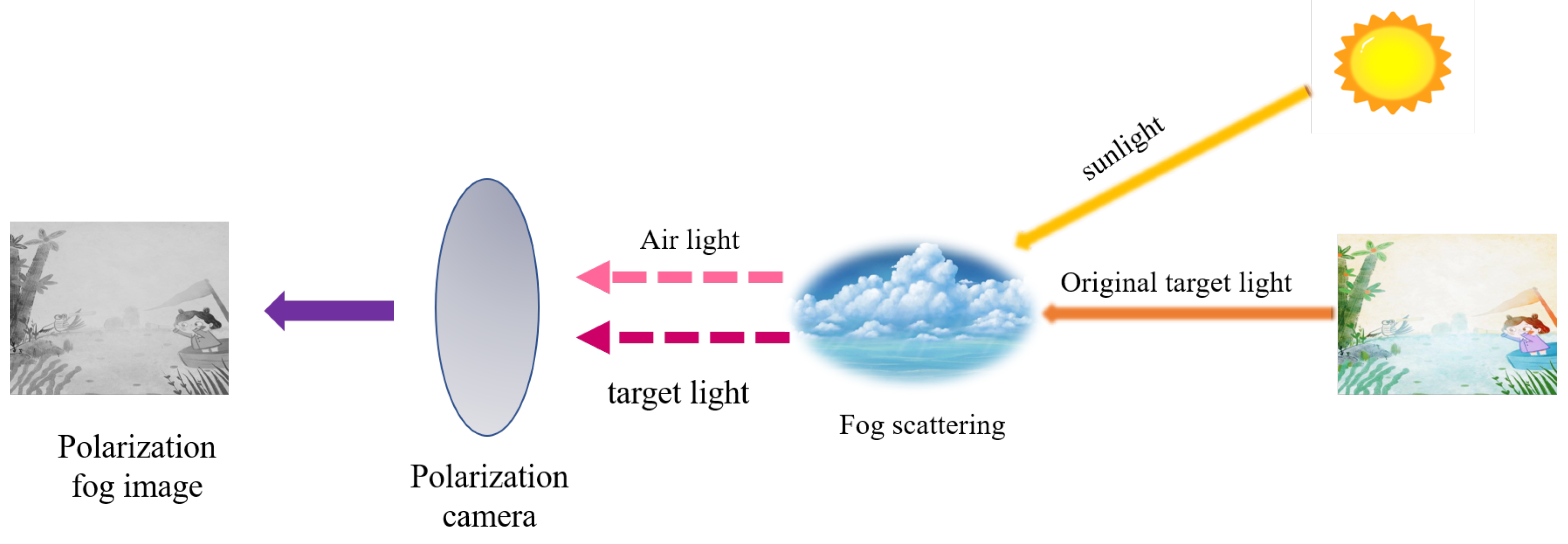
2.1. Atmospherical Scattering Model

In the field of image dehazing, common approaches include the Retinex-based dehazing enhancement model inspired by the human visual system (HVS) [29], as well as diffusion models integrated with deep learning. Among these, the atmospheric scattering model proposed by McCartney remains one of the most widely adopted frameworks for describing and processing haze-induced image degradation [30]. As illustrated in Figure 1, under this model, the light received by the detector is decomposed into two components:

• Attenuated target radiance: Light reflected from the target that is weakened through scattering and absorption by suspended particles in the atmosphere.
• Atmospheric light: Ambient light scattered by fog droplets, which dominates under dense haze conditions.

In heavy fog, the transmittance (fraction of light reaching the detector) decreases significantly. This causes the attenuated target radiance to become far weaker than the atmospheric light, ultimately submerging the target’s optical information within the overpowering airlight component.

$$I=D+A=Lt+A_{\infty }(1-t)$$

(1)

In Equation (1), I represents the foggy image captured by the detector; D represents the directly transmitted light; A represents the atmospheric light; $A_{\infty }$ is the atmospheric light intensity at an infinite distance. t represents transmittance. By rearranging Equation (1), the radiance of the haze-free image can be derived as:

$$L={\displaystyle \frac{I-A_{\infty }(1-t)}{t}}$$

(2)

2.2. Stokes Vector

The Stokes vector is a fundamental tool for describing the polarization state of light, comprehensively characterizing its polarization properties. In natural environments, polarized light is predominantly linearly polarized, with circular polarization components typically negligible. Therefore, by capturing four images ($I\left(0\right),I\left(45\right),I\left(90\right),I\left(135\right)$) at specific polarization angles (0°, 45°, 90°, 135°) using a polarimetric camera or rotating polarizer, we can compute the Stokes vector components as follows:

$$\begin{array}{cc}\hfill S& =\left(I\right(0)+I(45)+I(90)+I(135\left)\right)/2\hfill \\ \hfill S_1& =I\left(0\right)-I\left(90\right)\hfill \\ \hfill S_2& =I\left(45\right)-I\left(135\right)\hfill \end{array}$$

(3)

In the Equation (3), S represents the total light intensity, and $S_1$ represents the intensity difference between the 0° and 90° directions; $S_2$ is the intensity difference between the 45° direction and the 135° direction.

According to Malus’s theorem, the light intensity values for different polarization directions are given by Equation (4).

$$\begin{array}{cc}\hfill I_0& ={\displaystyle \frac{1}{2}}S(1-p)+Sp{\cos }^2(\theta -0^{\circ })\hfill \\ \hfill I_{45}& ={\displaystyle \frac{1}{2}}S(1-p)+Sp{\cos }^2(\theta -{45}^{\circ })\hfill \\ \hfill I_{90}& ={\displaystyle \frac{1}{2}}S(1-p)+Sp{\cos }^2(\theta -{90}^{\circ })\hfill \\ \hfill I_{135}& ={\displaystyle \frac{1}{2}}S(1-p)+Sp{\cos }^2(\theta -{135}^{\circ })\hfill \end{array}$$

(4)

Here, p is the degree of polarization (DoP) and $\theta$ is the angle of polarization (AoP). Using Malus’s theorem and the Stokes vector, the degree of polarization and polarization angle in the detected light can be determined, as shown in Equations (5) and (6).

$$p={\displaystyle \frac{\sqrt{{S_1}^2+{S_2}^2}}{S}}(0<p<1)$$

(5)

$$\begin{array}{cc}\hfill \theta =& {\displaystyle \frac{1}{2}}arctan{\displaystyle \frac{S_2}{S_1}}\hfill \\ \hfill (S2>0, S1& >0)\theta \in (0, {\displaystyle \frac{\pi }{4}})\hfill \\ \hfill (S2>0, S1& <0)\theta \in ({\displaystyle \frac{\pi }{4}}, {\displaystyle \frac{\pi }{2}})\hfill \\ \hfill (S2<0, S1& <0)\theta \in ({\displaystyle \frac{\pi }{2}}, {\displaystyle \frac{3\pi }{4}})\hfill \\ \hfill (S2<0, S1& >0)\theta \in ({\displaystyle \frac{3\pi }{4}}, \pi )\hfill \end{array}$$

(6)

2.3. Transmittance Estimation

As illustrated in Figure 2, through comparative analysis of numerous haze-free images across diverse scenes, we observed that targets typically exhibit distinct polarization characteristics, which accurately reflect their intrinsic properties. In contrast, sky regions demonstrate significantly weaker polarization properties, often orders of magnitude lower than those of targets. Building upon this theoretical prior, we propose that the polarization information acquired in foggy conditions arises from the combined contributions of target radiance and atmospheric light. By integrating this insight with the atmospheric scattering model, we derive the following key Equation (7):

$$S(1-p)=A_{\infty }(1-t)(1-p_A)+L(1-p_L)t$$

(7)

S is the light intensity obtained by the detector. $A_{\infty }$ is the intensity of light at infinity. L is the intensity of the target light. t is the transmittance. $p_A$ is the polarization degree of air light, and $p_L$ is the polarization degree of target light. p is the polarization degree of the probe light.

By rearranging Equation (7), we derive an expression for transmittance t, as shown in Equation (8). To address the challenge of estimating transmittance in heavy fog, this paper proposes a method that leverages the polarization properties of both target radiance and atmospheric light while incorporating boundary constraints to achieve robust estimation of t.

$$t={\displaystyle \frac{A_{\infty }(1-p_A)-S(1-p)}{A_{\infty }(1-p_A)-L(1-p_D)}}$$

(8)

In images, regions are not uniformly affected by fog. Fog-covered areas exhibit low transmittance. To maximize the recovery of target radiance, it is necessary to estimate the minimum transmittance. Due to fog-induced scattering, the polarization component of detected light is typically smaller than that of the target radiance (as $Sp<L{p}_D$). By scaling Equation (8) and leveraging scene similarity priors, we compute the minimum target radiance and derive the minimum transmittance for sky regions, as formalized in Equation (9). Conversely, fog-free regions exhibit higher transmittance, where atmospheric light contributes minimally. To preserve the fidelity of target radiance, we estimate the maximum transmittance. In clear conditions (as $Sp\approx L{p}_D$), maximizing the target radiance allows us to determine the maximum transmittance for non-sky regions, as shown in Equation (10).

$$t_{min}={\displaystyle \frac{A_{\infty }(1-p_A)-S(1-p)}{A_{\infty }(1-p_A)+Sp-L_{min}}}$$

(9)

$$t_{max}={\displaystyle \frac{A_{\infty }(1-p_A)-S(1-p)}{A_{\infty }(1-p_A)+Sp-L_{max}}}$$

(10)

where $L_{max}$ represents the maximum value of the target light, and $L_{min}$ represents its minimum value. $t_{max}$ represents the maximum transmittance, and $t_{min}$ represents its minimum value.

3. Experiment and Results

As illustrated in Figure 3, this paper first captures polarized images under foggy conditions across various scenes using a polarization camera as raw data for processing. Subsequently, threshold segmentation and fusion are applied to images at different scales to distinguish fog-affected areas from fog-free regions. The scope of the light intensity region at infinity is then determined to calculate both the light intensity value and atmospheric polarization degree at infinity. By leveraging the extreme values of target light in fog-free regions for boundary constraints, the transmittance is estimated, ultimately achieving image dehazing. Next, this section will provide a detailed explanation of the algorithm proposed in this article.

To conduct data collection across multiple scenarios under foggy conditions, this study employs a polarization camera model OR-250CNC-P for image acquisition. As depicted in Figure 4a, the polarization camera outputs images with a resolution of 2448 × 2048 pixels. Within the camera sensor, adjacent pixels are arranged in a 2 × 2 configuration, corresponding to the output polarization image information. The resulting images for different polarization components have a resolution of 1224 × 1024 pixels. The lens used for this data collection was a standard 50 mm fixed-focus lens, shown in Figure 4b. The camera was secured using a tripod and pan-tilt head, constructing a stable imaging platform illustrated in Figure 5, ensuring maximum precision in data acquisition under foggy conditions. The IDE used in this study is Microsoft Visual Studio, with C++ as the programming language, utilizing OpenCV for image processing operations.

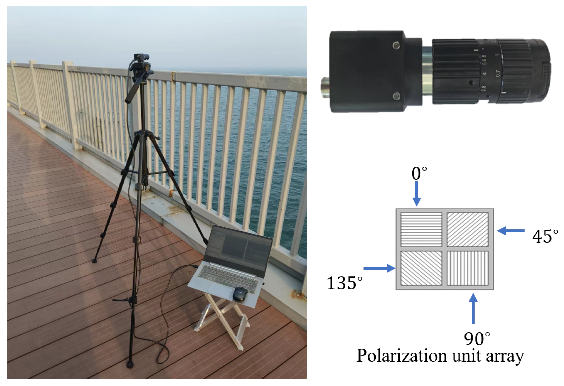
3.1. Data Preprocessing

Following data acquisition, image preprocessing is performed through a two-step procedure:

• Demultiplexing the raw images into distinct polarization-direction components via the polarization unit array.
• Calculating light intensity values and DoP using Equation (5).

As shown in Figure 6, the light intensity maps under different scenarios are presented

As shown in Figure 7, the DoP maps under different scenarios are presented

To further analyze the light intensity and polarization information, we compare the grayscale histograms derived from the intensity maps and DoP maps. As shown in Figure 8, displaying intensity histograms across different scenarios, it can be observed that under foggy conditions, the light intensity values typically exhibit multi-peak distributions with uneven grayscale allocation, leading to suboptimal performance in direct threshold segmentation.

As illustrated in Figure 9, analysis of grayscale histograms for the DoP across diverse scenarios reveals that polarization maps consistently exhibit distinct bimodal distributions. This indicates that polarization information, compared to light intensity data, enables more effective discrimination between background and target regions. In foggy conditions, this phenomenon manifests as a clear separation between haze-affected areas and haze-free areas.

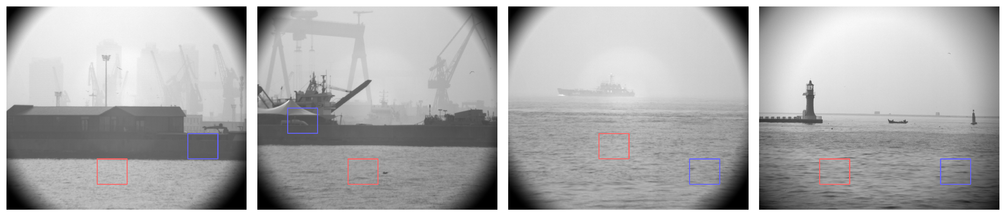
3.2. Determine the Atmospheric Light Intensity Value at Infinity

Accurately determining the atmospheric light intensity at infinity is a critical step in transmittance estimation and dehazing. Conventional methods typically select the maximum intensity value in the image as the atmospheric light, but this approach is prone to significant errors. To achieve more precise localization of sky regions, this paper proposes a multi-scale threshold fusion method to robustly estimate the atmospheric light intensity at infinity.

As shown in Figure 8, under foggy conditions, the gray-level distribution of light intensity information typically does not exhibit a bimodal histogram. In such similar scenarios, the background and objects are challenging to segment. However, since polarization characteristics are determined by the intrinsic properties of objects themselves, polarization information enables clear distinction between background and objects, as illustrated in Figure 9. Therefore, we adopt the OTSU method—a maximum inter-class variance threshold segmentation technique. This approach divides the image into background and object regions based on gray-level features. A larger inter-class variance between the gray values of these two regions indicates greater dissimilarity in composition and lower misclassification probability.

As shown in Figure 10, within the polarization domain, atmospheric regions exhibit comparatively low DoP relative to target regions, demonstrating distinct segmentation characteristics. Concurrently, according to the atmospheric scattering model, in the intensity domain, atmospheric regions typically display higher intensity values than target regions. To leverage these properties, we perform threshold-based binary segmentation on the polarization and intensity images, yielding distinct regional classifications as illustrated in Figure 10: Figure 10a: Intensity Threshold Segmentation Map; Figure 10b: DoP Threshold Segmentation Map.

Based on this, we define atmospheric regions as areas where the intensity segmentation map is white and the polarization degree segmentation map is black, with other regions classified as non-atmospheric. The final result is shown in Figure 10c. By selecting the maximum window-averaged intensity of the white regions in Figure 10c as the light intensity value at infinity $A_{\infty }^{\prime }$, and further ensuring robustness, we introduce a coefficient $A_{\infty }=\sigma A_{\infty }^{\prime }$. The finalized light intensity at infinity is then determined as $A_{\infty }$.

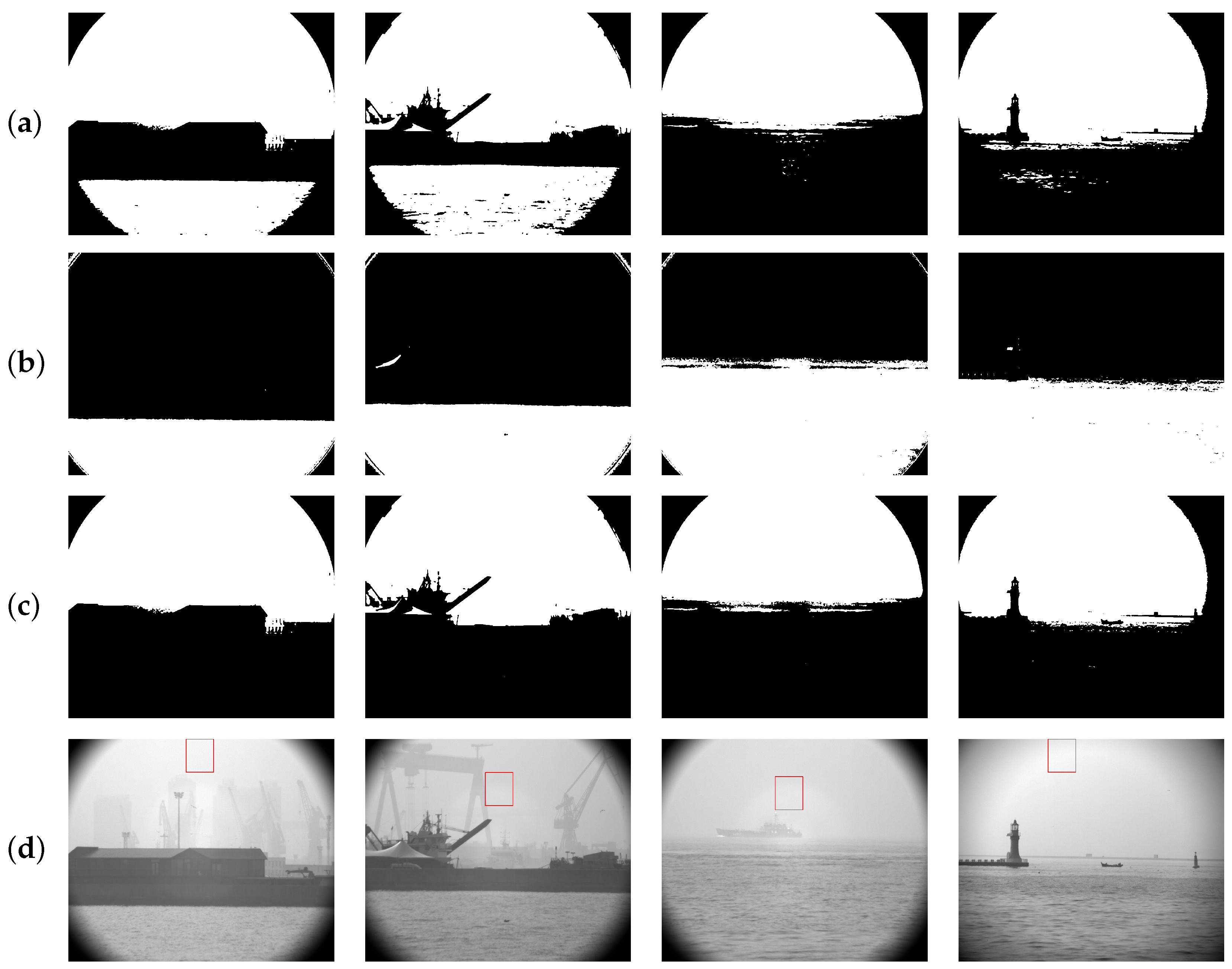
3.3. Boundary Constraints Based on Non Sky Region Light Intensity Values

According to Equations (9) and (10), the key to solving the maximum and minimum transmittance lies in determining the maximum and minimum values of the target radiance. In most scenarios, fog does not uniformly occlude all pixels in an image. Certain target regions remain unobscured by haze. As shown in Figure 10c, black areas represent non-occluded target regions. Leveraging the similarity of target radiance within the same scene, we select the maximum and minimum window-averaged values of the target radiance from these black regions as its extremal values. As illustrated in Figure 11, red boxes mark regions for calculating the maximum target radiance, while blue boxes denote regions for the minimum target radiance.

3.4. Calculate Transmittance

After obtaining the maximum and minimum target radiance values, we estimate the maximum and minimum transmittance using Equations (9) and (10). Since transmittance inherently ranges between 0 and 1, we further refine its bounds through Equation (11), as shown in Figure 12a,b. Regions occluded by dense fog exhibit relatively low transmittance, while unobscured regions show higher transmittance. Based on this principle, we assign minimum transmittance ($t_{\min }$) to white regions and maximum transmittance ($t_{\max }$) to black regions in the final segmentation map (Figure 12c). To further reduce errors, we apply mean filtering, yielding the refined transmittance map in Figure 12d.

$$\begin{array}{cc}\hfill t_{min}& =min(t_{min},1)\hfill \\ \hfill t_{max}& =min(t_{max},1)\hfill \end{array}$$

(11)

3.5. Calculate Target Light

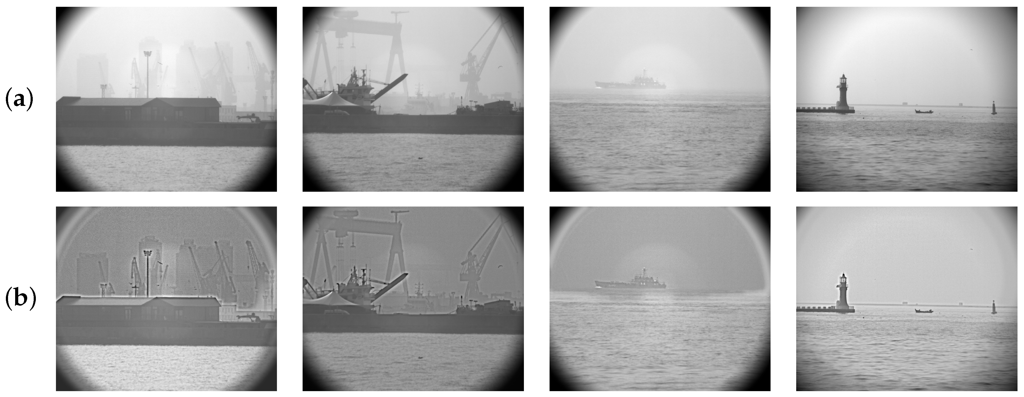
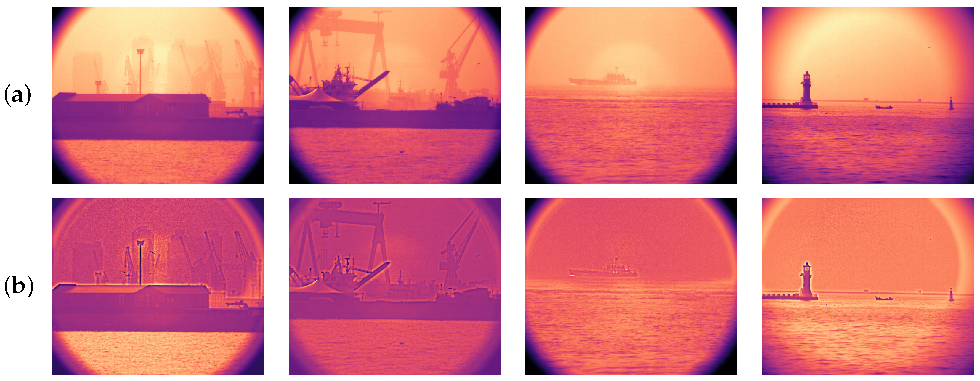
After obtaining the transmittance, we recover the final haze-free target radiance image using the atmospheric scattering model in Equation (2). As shown in Figure 13: Figure 13a is Original intensity image. Figure 13b is Dehazed intensity image.

Through visual comparison of light intensity images and their dehazed counterparts across various scenarios, it is evident that the optical information of targets obscured by fog has been effectively restored. In Scenarios 1 and 2, the building structures concealed by heavy fog demonstrate significant recovery. In Scenario 3, vessels submerged in dense fog become clearly identifiable. In Scenario 4, our algorithm efficiently eliminates light fog, successfully revealing target information.

4. Result Analysis

To facilitate a more comprehensive analysis of the experimental results, we applied pseudo-color mapping to Figure 14a, enabling more intuitive visual comparisons (see Figure 14b). In the intensity maps, the interference of atmospheric light with the target radiance under foggy conditions is clearly visible. Using the proposed dehazing algorithm, a significant improvement in image contrast is observed, and the target radiance obscured by atmospheric light is effectively recovered.

To objectively evaluate image quality, we employ four metrics: information entropy, average gradient, image standard deviation, and SSIM (Structural Similarity Index). Information entropy quantifies the amount of information in an image. Higher values indicate richer information content. Average gradient reflects the rate of fine-detail contrast variation, serving as an indicator of image sharpness [31]. Image standard deviation measures the dispersion of pixel values from the mean. Larger values suggest clearer edges and higher contrast [32]. SSIM assesses similarity between two images across three dimensions: luminance, contrast, and structure [33]. As shown in

Table 1. Dehazed Image Evaluation Metrics Table.

	Algorithm	Information Entropy	Average Gradient	Standard Deviation	SSMI
Scenario 1	Equalization	7.0618	21.0541	74.7433	0.7938
	Tradional	6.0503	22.6988	57.5973	0.2491
	Ours	7.2803	23.8238	37.6737	0.7959
Scenario 2	Equalization	7.0639	23.7906	74.8634	0.8125
	Tradional	6.5632	18.6107	58.9985	0.4558
	Ours	6.8527	16.3776	18.7265	0.8884
Scenario 3	Equalization	6.6994	37.9909	75.0269	0.6617
	Tradional	6.2549	24.9865	66.4276	0.4091
	Ours	7.0238	29.5858	28.8814	0.813691
Scenario 4	Equalization	7.2683	26.6495	73.8097	0.7970
	Tradional	6.2721	18.7083	57.7610	0.6676
	Ours	6.7742	21.8333	12.0983	0.9191

, the proposed algorithm achieves high information entropy and average gradient while maintaining maximum structural similarity (SSIM). These results validate the effectiveness of our dehazing method in enhancing image clarity and preserving critical details.

A comparative analysis of the proposed algorithm with histogram equalization and traditional dehazing algorithms is shown in Figure 15. Conventional polarization-based dehazing algorithms, which assume all polarization information originates from atmospheric light, exhibit significant limitations. In regions with high polarization degrees, this assumption leads to substantial errors, causing pixel value overflow and resulting in dark artifacts in the output images. Moreover, these methods demonstrate limited effectiveness in heavy fog conditions and yield images with suboptimal contrast. Histogram equalization is typically used to enhance the global contrast of many images, especially when the contrast of regions of interest is relatively low. This method allows brightness to be distributed more evenly across the histogram. Consequently, it can improve local contrast without affecting the overall contrast. However, though histogram equalization enhances details of objects in foggy conditions, the visual improvement is often not significant. In contrast, the proposed algorithm achieves significant enhancement in target contrast while avoiding the pixel overflow issues inherent to traditional polarization-based dehazing methods. It effectively removes haze while preserving structural similarity to the greatest extent possible, ensuring natural and artifact-free results.

5. Conclusions and Prospect

This paper proposes a dehazing algorithm based on joint polarimetric transmittance estimation via multi-scale segmentation and fusion and demonstrates robust dehazing performance across diverse multi-target scenarios. First, by fusing polarization cues and intensity cues, we achieve highly accurate sky region localization, establishing a critical foundation for subsequent processing. Second, haze-occluded regions and haze-free regions are identified through joint intensity-polarization threshold segmentation. Spatially adaptive transmittance estimation is then performed for each region using corresponding algorithms. This framework enables high-quality dehazing while maximizing structural similarity preservation. Despite the algorithm’s effectiveness in haze removal and image enhancement, certain limitations remain. Future work will focus on addressing these constraints to further refine performance.

• This method depends on selecting sky regions to estimate the atmospheric polarization degree ($p_A$) and atmospheric light intensity at infinity ($A_{\infty }$). For sky-free images, we are forced to rely on empirical priors for estimation, which may introduce significant estimation errors in specific scenarios.
• This approach heavily relies on the accuracy of image segmentation and fusion. In certain scenarios, visibly unnatural boundaries may emerge during segmentation and fusion, or inaccurate region classification may occur, leading to distorted boundaries. Future enhancements may involve employing semantic segmentation and salient object detection methodologies to further improve segmentation diversity and accuracy, thereby strengthening the algorithm’s robustness.
• There is still room for optimization in determining the boundary values of the target light in this article in order to make the estimation of transmittance more accurate and the dehazing effect better.

References

1. Ancuti, C.O.; Ancuti, C.; Timofte, R.; Vleeschouwer, C.D. I-HAZE: A dehazing benchmark with real hazy and haze-free indoor images. arXiv 2018, arXiv:1804.05091. [Google Scholar] [CrossRef]
2. Singh, D.; Chahar, V. A Comprehensive Review of Computational Dehazing Techniques. Arch. Comput. Methods Eng. 2018, 26, 1395–1413. [Google Scholar] [CrossRef]
3. Yeh, C.H.; Kang, L.W.; Lee, M.S.; Lin, C.Y. Haze effect removal from image via haze density estimation in optical model. Opt. Express 2013, 21, 27127–27141. [Google Scholar] [CrossRef] [PubMed]
4. Liu, J.; Wang, X.; Chen, M.; Liu, S.; Zhou, X.; Shao, Z.; Liu, P. Thin cloud removal from single satellite images. Opt. Express 2014, 22, 618–632. [Google Scholar] [CrossRef]
5. He, K.; Sun, J.; Tang, X. Single Image Haze Removal Using Dark Channel Prior. IEEE Trans. Pattern Anal. Mach. Intell. 2011, 33, 2341–2353. [Google Scholar] [CrossRef]
6. Lee, S.; Yun, S.; Nam, J.H.; Won, C.; Jung, S.W. A review on dark channel prior based image dehazing algorithms. EURASIP J. Image Video Process. 2016, 2016, 4. [Google Scholar] [CrossRef]
7. Li, Z.X.; Wang, Y.L.; Peng, C.; Peng, Y. Laplace dark channel attenuation-based single image defogging in ocean scenes. Multim. Tools Appl. 2023, 82, 21535–21559. [Google Scholar] [CrossRef]
8. Wang, S.; Yang, T.; Sun, W.; Lu, X.; Fan, D. Adaptive Bright and Dark Channel Combined with Defogging Algorithm Based on Depth of Field. J. Sens. 2022, 2022. [Google Scholar] [CrossRef]
9. Fang, Z.; Wu, Q.; Huang, D.; Guan, D. An Improved DCP-Based Image Defogging Algorithm Combined with Adaptive Fusion Strategy. Math. Probl. Eng. 2021, 2021. [Google Scholar] [CrossRef]
10. Ancuti, C.; Ancuti, C.O.; Haber, T.; Bekaert, P. Enhancing underwater images and videos by fusion. In Proceedings of the 2012 IEEE Conference on Computer Vision and Pattern Recognition, Providence, RI, USA, 16–21 June 2012; pp. 81–88. [Google Scholar] [CrossRef]
11. Chen, T.; Liu, M.; Gao, T.; Cheng, P.; Mei, S.; Li, Y. A Fusion-Based Defogging Algorithm. Remote Sens. 2022, 14, 425. [Google Scholar] [CrossRef]
12. He, S.; Chen, Z.; Wang, F.; Wang, M. Integrated image defogging network based on improved atmospheric scattering model and attention feature fusion. Earth Sci. Inform. 2021, 14, 2037–2048. [Google Scholar] [CrossRef]
13. Cai, B.; Xu, X.; Jia, K.; Qing, C.; Tao, D. DehazeNet: An End-to-End System for Single Image Haze Removal. IEEE Trans. Image Process. 2016, 25, 5187–5198. [Google Scholar] [CrossRef]
14. Zhang, H.; Patel, V.M. Densely Connected Pyramid Dehazing Network. In Proceedings of the 2018 IEEE/CVF Conference on Computer Vision and Pattern Recognition, Salt Lake City, UT, USA, 18–23 June 2018; pp. 3194–3203. [Google Scholar] [CrossRef]
15. Kumar, R.; Kaushik, B.K.; Raman, B.; Sharma, G. A Hybrid Dehazing Method and its Hardware Implementation for Image Sensors. IEEE Sens. J. 2021, 21, 25931–25940. [Google Scholar] [CrossRef]
16. Li, Z.X.; Wang, Y.L.; Peng, C. MIDNet: A Weakly Supervised Multipath Interaction Network for Image Defogging. In Proceedings of the 2024 36TH Chinese Control and Decision Conference, CCDC, Xi’an, China, 25–27 May 2024. [Google Scholar] [CrossRef]
17. Song, Y.; Zhao, J.; Shang, C. A multi-stage feature fusion defogging network based on the attention mechanism. J. Supercomput. 2024, 80, 4577–4599. [Google Scholar] [CrossRef]
18. Ma, T.; Zhou, J.; Zhang, L.; Fan, C.; Sun, B.; Xue, R. Image Dehazing With Polarization Boundary Constraints of Transmission. IEEE Sens. J. 2024, 24, 12971–12984. [Google Scholar] [CrossRef]
19. Liu, S.; Li, H.; Zhao, J.; Liu, J.; Zhu, Y.; Zhang, Z. Atmospheric Light Estimation Using Polarization Degree Gradient for Image Dehazing. Sensors 2024, 24, 3137. [Google Scholar] [CrossRef] [PubMed]
20. Ma, R.; Zhang, Z.; Zhang, S.; Wang, Z.; Liu, S. A Polarization-Based Method for Maritime Image Dehazing. Appl. Sci. 2024, 14, 4234. [Google Scholar] [CrossRef]
21. Schechner, Y.; Narasimhan, S.; Nayar, S. Instant dehazing of images using polarization. In Proceedings of the 2001 IEEE Computer Society Conference on Computer Vision and Pattern Recognition. CVPR 2001, Kauai, HI, USA, 8–14 December 2001; Volume 1, pp. I–I. [Google Scholar] [CrossRef]
22. Liang, J.; Ren, L.; Ju, H.; Qu, E.; Wang, Y. Visibility enhancement of hazy images based on a universal polarimetric imaging method. J. Appl. Phys. 2014, 116, 173107. [Google Scholar] [CrossRef]
23. Liang, J.; Ren, L.; Qu, E.; Hu, B.; Wang, Y. Method for enhancing visibility of hazy images based on polarimetric imaging. Photon. Res. 2014, 2, 38–44. [Google Scholar] [CrossRef]
24. Liang, J.; Ren, L.; Ju, H.; Qu, E. Polarimetric dehazing method for dense haze removal based on distribution analysis of angle of polarization. Opt. Express 2015, 23, 26146–26157. [Google Scholar] [CrossRef] [PubMed]
25. Liang, J.; Zhang, W.; Ren, L.; Ju, H.; Qu, E. Polarimetric dehazing method for visibility improvement based on visible and infrared image fusion. Appl. Opt. 2016, 55, 8221–8226. [Google Scholar] [CrossRef]
26. Teurnier, B.L.; Tullio, A.; Boffety, M. Enhancing the robustness of underwater dehazing by jointly using polarization and the dark channel prior. Appl. Opt. 2025, 64, 5195–5205. [Google Scholar] [CrossRef]
27. Fang, S.; Xia, X.; Huo, X.; Chen, C. Image dehazing using polarization effects of objects and airlight. Opt. Express 2014, 22, 19523–19537. [Google Scholar] [CrossRef]
28. Sun, C.; Ding, Z.; Ma, L. Optimized method for polarization-based image dehazing. Heliyon 2023, 9, e15849. [Google Scholar] [CrossRef] [PubMed]
29. Kim, K.; Bae, J.; Kim, J. Natural hdr image tone mapping based on retinex. IEEE Trans. Consum. Electron. 2011, 57, 1807–1814. [Google Scholar] [CrossRef]
30. McCartney, E.J. Optics of the Atmosphere: Scattering by Molecules and Particles; John Wiley & Sons Inc.: Hoboken, NJ, USA, 1976. [Google Scholar]
31. Di Zenzo, S. A note on the gradient of a multi-image. Comput. Vision Graph. Image Process. 1986, 33, 116–125. [Google Scholar] [CrossRef]
32. Chang, D.C.; Wu, W.R. Image contrast enhancement based on a histogram transformation of local standard deviation. IEEE Trans. Med. Imaging 1998, 17, 518–531. [Google Scholar] [CrossRef]
33. Horé, A.; Ziou, D. Image Quality Metrics: PSNR vs. SSIM. In Proceedings of the 2010 20th International Conference on Pattern Recognition, Istanbul, Turkey, 23–26 August 2010; pp. 2366–2369. [Google Scholar] [CrossRef]
Figure 1. Atmospheric scattering model diagram.
Applsci 15 08632 g001
Figure 2. DoP Map under clear conditions.
Applsci 15 08632 g002
Figure 3. Flow chat of dehazing algorithm based on joint polarimetric transmittance estimation via multi-scale segmentation and fusion.
Applsci 15 08632 g003
Figure 4. Polarization camera and fixed focus lens. (a): Polarization camera; (b): focus lens.
Applsci 15 08632 g004
Figure 5. Data Acquisition Setup and Pixel Arrangement Diagram.
Applsci 15 08632 g005
Figure 6. Intensity maps in different scenarios.
Applsci 15 08632 g006
Figure 7. DoP maps in different scenarios.
Applsci 15 08632 g007
Figure 8. DoP maps in different scenarios.
Applsci 15 08632 g008
Figure 9. DoP maps in different scenarios.
Applsci 15 08632 g009
Figure 10. Segmentation maps under different scenarios: intensity threshold, DoP threshold, fused threshold, and sky region identification. (a): Intensity Threshold Segmentation Map; (b): DoP Threshold Segmentation Map; (c): Fused Threshold Segmentation Map; (d): Identified Sky Region Map.
Applsci 15 08632 g010
Figure 11. Target light selection Map in different scenarios.
Applsci 15 08632 g011
Figure 12. Pseudo-color maps of transmittance under different scenarios: (a): Minimum transmittance pseudo-color map; (b): Maximum transmittance pseudo-color map; (c): Transmittance pseudo-color map; (d): Filtered transmittance pseudo-color map.
Applsci 15 08632 g012
Figure 13. Intensity images and dehazed intensity images under different scenarios: (a) Original intensity image; (b) Dehazed intensity image.
Applsci 15 08632 g013
Figure 14. Pseudo color images of light intensity and final pseudo color images in different scenarios: (a) Intensity pseudo color image; (b) Final pseudo color image.
Applsci 15 08632 g014
Figure 15. Intensity images and dehazing results under different scenarios using various methods: (a): Intensity image; (b): Histogram equalization; (c): Traditional polarization-based dehazing; (d): Proposed algorithm.
Applsci 15 08632 g015aApplsci 15 08632 g015b