Characterization of Spatial Variability in Rock Mass Mechanical Parameters for Slope Stability Assessment: A Comprehensive Case Study

Abstract

The spatial variability in rock mass mechanical parameters critically affects slope stability assessments. This study investigated the southern slope of the Bayan Obo open-pit mine. A representative elementary volume (REV) with a side length of 14 m was determined through discrete fracture network (DFN) simulations. Based on the rock quality designation (RQD) data from 40 boreholes, a three-dimensional spatial distribution model of the RQD was constructed using Ordinary Kriging interpolation. The RQD values were converted into geological strength index (GSI) values through an empirical correlation, and the generalized Hoek–Brown criterion was applied to develop a spatially heterogeneous equivalent mechanical parameter field. Numerical simulations were performed using FLAC3D, with the slope stability evaluated using the point safety factor (PSF) method. For comparison, three homogeneous benchmark models based on the 5th, 25th, and 50th percentiles produced profile-scale safety factors of 0.96–1.92 and failed to replicate the observed failure geometry. By contrast, the heterogeneous model yielded safety factors of approximately 1.03–1.08 and accurately reproduced the mapped sliding surface. These findings demonstrate that incorporating spatial heterogeneity significantly improves the accuracy of slope stability assessments, providing a robust theoretical basis for targeted monitoring and reinforcement design.

1. Introduction

Slope rock masses are typically characterized by multiple joint sets and diverse lithologies, resulting in pronounced spatial heterogeneity [1,2,3]. First, the spatial distribution of rock mass properties—such as compressive strength, elastic modulus, and friction angle—varies due to mineral composition gradients, weathering processes, and tectonic deformation [4,5]. Second, the development of structural planes, including joints, fissures, and faults, introduces additional anisotropy and weak-plane effects [6,7]. These factors collectively lead to significant deviations in stress distribution and failure mechanisms compared with homogeneous assumptions. Neglecting or oversimplifying such spatial heterogeneity in slope stability analyses often results in underestimated hazard levels and inaccurately predicted failure extents, thereby compromising engineering safety and decision-making reliability [8,9].

To address this, researchers have extensively explored methods for characterizing the spatial variability in rock mass mechanical parameters and integrating them into slope stability assessments. Currently, two primary approaches are prevalent: geostatistics [10] and random field theory [11]. Originating from mineral resource estimation, geostatistics quantifies the spatial correlation of rock mass parameters through variogram analysis [11,12], enabling the construction of spatial distribution models via interpolation techniques, such as Ordinary Kriging [13]. Its notable applications include the simulation of Rock Mass Rating (RMR) spatial variability by Pinheiro et al. [14], and the estimation of geological strength index (GSI) distributions by Liu et al. [10].

Alternatively, random field theory treats rock mass parameters as spatially correlated random variables, typically assuming normal or lognormal distributions [15]. Random parameter fields are generated using methods such as Cholesky decomposition [16], Karhunen–Loève (K–L) expansion [17], and local average subdivision [18], and incorporated into finite element or finite difference models via Monte Carlo simulations [19]. Representative studies include Zhang et al.’s [4] investigation of weak-layer variability and seismic randomness effects and Chen et al.’s [20] development of cross-correlated non-Gaussian random fields for stratified rock masses.

While both approaches have established a solid foundation for the stability analysis of jointed rock masses [21,22], challenges remain, particularly for large-scale, highly heterogeneous open-pit slopes. Geostatistical methods typically treat the interpolated mechanical parameters as deterministic inputs [10], whereas random field models, though probabilistically robust, often entail significant computational costs, restricting their application to small- or medium-scale problems [23]. For example, Aminpour et al. [24] performed a full Monte Carlo simulation (MCS) with 120,000 three-dimensional finite-difference realizations, each containing an 800-cell mesh; the complete run consumed ≈ 306 CPU days (i.e., several hundred days of processor time), underscoring that reliability analyses of large study areas can demand enormous computational resources.

This study addresses these limitations by investigating the southern slope of the Bayan Obo open-pit mine using a high-resolution geostatistical approach. The proposed methodology involves four sequential phases: (1) determining the representative elementary volume (REV) through three-dimensional discrete fracture network (DFN) simulations; (2) constructing a spatial distribution model of rock quality designation (RQD) based on borehole exploration data via Ordinary Kriging interpolation; (3) integrating the generalized Hoek–Brown failure criterion to convert the rock mass quality indices into the equivalent mechanical parameters, thereby generating a spatially variable mechanical parameter field; and (4) evaluating the slope stability using the point safety factor method within a numerical FLAC3D framework.

2. Characterization of Spatial Variability and Slope Stability Assessment Methods

2.1. Ordinary Kriging Interpolation

In this study, the primary dataset comprises RQD measurements. The exploratory data analysis did not reveal a statistically significant large-scale drift in the RQD; therefore, a trend-based formulation, such as Universal Kriging, was not warranted. No independent, spatially co-extensive secondary variable was available, making co-Kriging inappropriate (the GSI employed later was derived from the RQD and is therefore not an independent covariate). In addition, the modeling domain was large and the numerical analysis used a high-resolution grid on the order of two million grid zones, so fully probabilistic alternatives (e.g., conditional simulation or random-field Monte Carlo coupling) would have required hundreds to thousands of realizations and were computationally impractical under our budget. Under these conditions, Ordinary Kriging provided an optimal linear unbiased estimator for the given sample set and yielded a reliable deterministic spatial model of RQD to support the subsequent mechanical parameterization and slope stability assessment [25]. The core methodology is based on the formulation and application of a semivariogram, mathematically expressed as follows:

$$\mathsf{\gamma }(h)={\displaystyle \frac{1}{2n(h)}}{\displaystyle \sum _{i=1}^{n(h)}{(X(z_i)-X(z_i+h))}^2}$$

(1)

where $X(z_i)$ and $X(z_i+h)$ denote the observed values at positions $z_i$ and $z_i+h$, respectively; $h$ represents the distance between these two points; and $n(h)$ is the number of sampling point pairs separated by distance $h$.

In practical applications, an experimental semivariogram’s data points are typically fitted to derive a mathematical model. Among the available models, the spherical model incorporating a nugget effect is the most widely utilized in practice. Its mathematical expression is as follows:

$$\mathsf{\gamma }(h)=\left\{\begin{array}{cc}N+C({\displaystyle \frac{3h}{2\mathsf{\beta }}}-{\displaystyle \frac{h^3}{2{\mathsf{\beta }}^3}})& h\le \mathsf{\beta }\\ N+C& h>\mathsf{\beta }\end{array}\right.$$

(2)

in which $N$ represents the nugget value, $C$ the sill value, and $\mathsf{\beta }$ the range. When the distance $h\le \mathsf{\beta }$, the spatial correlation decays nonlinearly with an increasing $h$. For $h>\mathsf{\beta }$, the spatial autocorrelation becomes negligible, and $\mathsf{\gamma }(h)$ approaches $(N+C)$, corresponding to the overall sample variance.

According to the theory of optimal estimation, the Kriging weights $w$ must satisfy both the unbiasedness condition and the minimum variance criterion. Their matrix expression is as follows:

$$\left[\begin{array}{c}{w}_1\\ w_2\\ ⋮\\ w_n\\ \mathsf{\lambda }\end{array}\right]={\left[\begin{array}{ccccc}{\mathsf{\gamma }}_{11}& {\mathsf{\gamma }}_{12}& \dots & {\mathsf{\gamma }}_{1n}& 1\\ {\mathsf{\gamma }}_{21}& {\mathsf{\gamma }}_{22}& \dots & {\mathsf{\gamma }}_{2n}& 1\\ ⋮& ⋮& \dots & ⋮& ⋮\\ {\mathsf{\gamma }}_{n1}& {\mathsf{\gamma }}_{n2}& \dots & {\mathsf{\gamma }}_{nn}& 1\\ 1& 1& \dots & 1& 0\end{array}\right]}^{-1}\left[\begin{array}{c}{\mathsf{\gamma }}_{01}\\ {\mathsf{\gamma }}_{02}\\ ⋮\\ {\mathsf{\gamma }}_{0n}\\ 1\end{array}\right]$$

(3)

where $n$ denotes the number of effective sampling points, ${\mathsf{\gamma }}_{0i}$ represents the semivariogram value between the point to be estimated and the $i$-th known point, and $\mathsf{\lambda }$ is the Lagrange multiplier. Solving this system of linear equations yields the optimal weight coefficients, enabling the predicted value of the point to be estimated to be expressed as follows:

$${\widehat{x}}_0={\displaystyle \sum _{i=1}^n{w}_i{x}_i}$$

(4)

2.2. Generalized Hoek–Brown Criterion

The generalized Hoek–Brown criterion is derived from extensive field tests and engineering practice. By incorporating empirical parameters that characterize rock mass properties, it establishes a quantitative correlation between the rock mass failure criterion and these parameters [26]. This criterion comprehensively accounts for both the geological characteristics and mechanical properties of rock masses, enabling the determination of equivalent mechanical parameters suitable for slope stability analysis. The mathematical expression of this criterion is as follows:

$${\mathsf{\sigma }}_1={\mathsf{\sigma }}_3+{\mathsf{\sigma }}_{ci}{\left(m_b{\displaystyle \frac{{\mathsf{\sigma }}_3}{{\mathsf{\sigma }}_{ci}}}+s\right)}^a$$

(5)

where ${\mathsf{\sigma }}_1$ and ${\mathsf{\sigma }}_3$ denote the maximum and minimum principal stresses (MPa) at failure, respectively; ${\mathsf{\sigma }}_{ci}$ represents the uniaxial compressive strength (MPa) of the intact rock; $m_b$ is an empirical parameter characterizing the rock mass, calculated using Equation (6); $s$ is the integrity coefficient of the rock mass, determined by Equation (7); and $a$ is a constant characterizing the jointed rock mass, as expressed in Equation (8).

$$m_b=\exp \left({\displaystyle \frac{GSI-100}{28-14D}}\right)m_i$$

(6)

$$s=\exp \left({\displaystyle \frac{GSI-100}{9-3D}}\right)$$

(7)

$$a=0.5+{\displaystyle \frac{1}{6}}\left[\exp \left(-{\displaystyle \frac{GSI}{15}}\right)-\exp \left(-{\displaystyle \frac{20}{3}}\right)\right]$$

(8)

in which $D\in [0,1]$ denotes the excavation disturbance coefficient of the rock mass; $m_i$ represents the rock hardness; and $GSI$ is the geological strength index of the rock mass, with its engineering estimation formula expressed as follows:

$$GSI=1.5JCon{d}_{89}+RQD/2$$

(9)

where $JCon{d}_{89}$ denotes the structural plane condition coefficient, while $RQD$ represents the rock quality designation, defined as the percentage of the cumulative length of intact rock core segments exceeding 10 cm in a core run relative to the total length of that core run.

The tensile strength ${\mathsf{\sigma }}_t$ (MPa) of the rock mass is given by the following equation:

$${\mathsf{\sigma }}_t={\displaystyle \frac{-s{\mathsf{\sigma }}_{ci}}{m_b}}$$

(10)

When ${\mathsf{\sigma }}_{ci}<100$ MPa, the deformation modulus $E_m$ of the rock mass can be approximated as follows:

$$E_m(GPa)=(1-{\displaystyle \frac{D}{2}})\sqrt{{\displaystyle \frac{{\mathsf{\sigma }}_{ci}}{100}}}{10}^{\left({\displaystyle \frac{GSI-10}{40}}\right)}$$

(11)

Based on the area equivalence principle, the optimal fitting parameters for approximating the Hoek–Brown curve using the Mohr–Coulomb linear criterion in Equation (5) are determined. The equivalent internal friction angle $\mathsf{\varphi }\prime$ (°) and equivalent cohesion $c\prime$ (MPa) of the rock mass are derived as follows:

$$\mathsf{\varphi }\prime ={\sin }^{-1}\left[{\displaystyle \frac{6\mathsf{\alpha }{m}_b{(s+m_b{\mathsf{\sigma }}_{3n}^{\prime })}^{\mathsf{\alpha }-1}}{2(1+\mathsf{\alpha })(2+\mathsf{\alpha })+6\mathsf{\alpha }{m}_b{(s+m_b{\mathsf{\sigma }}_{3n}^{\prime })}^{\mathsf{\alpha }-1}}}\right]$$

(12)

$$c\prime ={\displaystyle \frac{{\mathsf{\sigma }}_{ci}[(1+2\mathsf{\alpha })s+(1-\mathsf{\alpha })m_b{\mathsf{\sigma }}_{3n}^{\prime }]{(s+m_b{\mathsf{\sigma }}_{3n}^{\prime })}^{\mathsf{\alpha }-1}}{(1+\mathsf{\alpha })(2+\mathsf{\alpha })\sqrt{1+\frac{6\mathsf{\alpha }{m}_b{(s+m_b{\mathsf{\sigma }}_{3n}^{\prime })}^{\mathsf{\alpha }-1}}{(1+\mathsf{\alpha })(2+\mathsf{\alpha })}}}}$$

(13)

Here, ${\mathsf{\sigma }}_{3n}^{\prime }$ represents the ratio of the maximum confining pressure ${\mathsf{\sigma }}_{3\max }^{\prime }$ to the uniaxial compressive strength ${\mathsf{\sigma }}_{ci}$ of the rock block, and ${\mathsf{\sigma }}_{3\max }^{\prime }$ is calculated as follows:

$${\mathsf{\sigma }}_{3\max }^{\prime }=0.72{\mathsf{\sigma }}_{cm}{\left({\displaystyle \frac{{\mathsf{\sigma }}_{cm}}{\mathsf{\rho }H}}\right)}^{-0.91}$$

(14)

where $\mathsf{\rho }$ denotes the unit weight of the rock (MN/m³), $H$ represents the engineering burial depth (m), and ${\mathsf{\sigma }}_{cm}$ corresponds to the uniaxial compressive strength of the rock mass (MPa). The analytical expression for ${\mathsf{\sigma }}_{cm}$ is as follows:

$${\mathsf{\sigma }}_{cm}={\mathsf{\sigma }}_{ci}{\displaystyle \frac{\left[m_b+4s-a\left(m_b-8s\right)\right]{\left(\raisebox{1ex}{$m_b$}\!\left/ \!\raisebox{-1ex}{$4$}\right.+s\right)}^{a-1}}{2\left(1+a\right)\left(2+a\right)}}$$

(15)

2.3. Point Safety Factor Method

The point safety factor (PSF) method facilitates rapid assessment of overall slope stability through computation of local safety factors at multiple points within the slope mass [27,28]. Unlike the strength reduction method, which requires iterative calculations, this approach eliminates the need for repeated numerical trials, substantially enhancing the computational efficiency for large-scale, complex grid models. The local safety factor, denoted as $k$, is mathematically defined as follows:

$$k={\displaystyle \frac{{\mathsf{\sigma }}_n\tan \mathsf{\varphi }\prime +c\prime }{\mathsf{\tau }}}$$

(16)

where ${\mathsf{\sigma }}_n$ denotes the normal stress (kPa), $\mathsf{\tau }$ denotes the shear stress (kPa), $\mathsf{\varphi }\prime$ denotes the equivalent internal friction angle (°), and $c\prime$ denotes the equivalent cohesion (kPa). For a material point under a three-dimensional stress state (${\mathsf{\sigma }}_1$, ${\mathsf{\sigma }}_2$, ${\mathsf{\sigma }}_3$), with the direction cosines ($l$, $m$, $n$) defining the normal to the potential slip surface relative to the principal stress directions, the normal stress ${\mathsf{\sigma }}_n$ and shear stress $\mathsf{\tau }$ are given by the following:

$${\mathsf{\sigma }}_n=l^2{\mathsf{\sigma }}_1+m^2{\mathsf{\sigma }}_2+n^2{\mathsf{\sigma }}_3$$

(17)

$$\mathsf{\tau }=\sqrt{l^2{\mathsf{\sigma }}_1^2+m^2{\mathsf{\sigma }}_2^2+n^2{\mathsf{\sigma }}_3^2-{\mathsf{\sigma }}_n^2}$$

(18)

A schematic diagram illustrating the PSF method is presented in Figure 1. Given the typical stress characteristics in slope engineering and noting that the direction of the intermediate principal stress ${\mathsf{\sigma }}_2$ is approximately orthogonal to the potential slip surface’s normal vector, it is reasonable to set $m\approx 0$. Under this condition, the direction cosines $l$ and $n$ can be derived from the following expressions:

$$l=\sqrt{1-n^2}$$

(19)

$$n=\pm \sqrt{{\displaystyle \frac{{\mathsf{\sigma }}_1\tan \mathsf{\varphi }\prime +c\prime }{({\mathsf{\sigma }}_1+{\mathsf{\sigma }}_3)\tan \mathsf{\varphi }\prime +2c\prime }}}$$

(20)

To validate the PSF method, we conducted a comparative analysis of safety factor (Fs) results and those obtained with the conventional shear strength reduction (SSR) approach (Figure 2). When the rock mass strength is largely unreduced (Figure 2a), low Fs zones develop only locally. After the strength is reduced to Fs ≈ 1.0 (Figure 2b), the PSF-derived low Fs band coincides with both the maximum shear strain zone predicted by the SSR analysis (Figure 2c) and the corresponding plastic zone (Figure 2d). The overall factor of safety for Figure 2b, computed with the SSR, is Fs = 0.97—essentially identical to the minimum Fs ≈ 1.0 on the PSF map—demonstrating the consistency of the two methods at the limit equilibrium stage.

3. Engineering Case Study

3.1. Engineering Overview

The Bayan Obo open-pit mine is located in Baotou City, Inner Mongolia Autonomous Region, China (Figure 3a). The primary mining area spans approximately 1620 m in length and 1140 m in width, exhibiting a predominantly east–west orientation. Engineering geological investigations have indicated that the southern slope of the main mining area comprises four distinct lithological units: slate, dolomite, limestone, and mica schist (Figure 3b).

On 29 August 2020, a landslide occurred on the southern slope of the main mining area at the Bayan Obo open-pit mine (Figure 4a). Field investigations and measurements revealed that the landslide’s trailing edge was exposed at the 1650 m platform, extending approximately 500 m in length. The leading edge shear outlet was positioned at the 1542 m level, with the displaced material ultimately accumulating on the 1458 m platform. A geometric analysis of the landslide mass indicated a maximum north–south horizontal width of 55 m, a projected area of 1.23 × 10⁴ m², and an estimated total volume of approximately 9.2 × 10⁵ m³. This failure was driven by the combined effects of a poorly confined convex slope face, multiple intersecting faults that weakened the rock mass, and long-term bench excavation that progressively reduced stability.

A regional tectonic analysis (Figure 4b) revealed well-developed fault structures within the landslide area, characterized by predominantly east–west striking faults with dip angles exceeding 60° and individual fault thicknesses ranging from 5 to 30 m. These reverse-dipping fault structures, particularly their intersecting patterns, significantly compromised slope stability through their synergistic effects.

A high-density resistivity survey was performed on the 1650 m platform, with the results illustrated in Figure 5. The southern slope displays exceptionally thick weathered material, extending to a maximum depth of 50 m, and exhibits localized fracture zones. An engineering geological analysis indicated that the rock mass exhibits “double-weakness” characteristics—manifesting highly developed structural planes and comparatively low mechanical parameters. These conditions represent significant intrinsic factors contributing to slope instability.

3.2. Determination of Representative Volume Element Size

In numerical simulation studies, selection of REV dimensions critically impacts both the computational efficiency and simulation reliability [29]. This study developed a three-dimensional DFN model to investigate the size effects in fractured rock masses, with the objective of determining the optimal REV dimensions for the study area.

A representative area of the 1542 m platform on the southern slope of the main mining area—distinguished by well-exposed strata and extensively developed joint systems (Figure 4a)—was selected for analysis. The slope point cloud data were acquired through Unmanned Aerial Vehicle oblique photogrammetry. We utilized an integrated analytical approach (including normal vector calculations, octree segmentation, Fuzzy C-Means clustering, and DBSCAN) to analyze the point cloud data [30]. Three dominant joint sets, comprising 488 individual joints, were identified (Figure 6).

A statistical analysis of the joint geometric parameters (Figure 7) revealed the following: Joint Set 1 intersects the slope surface obliquely and exhibits the longest average trace length (2.44 m) among the three joint sets. Joint Set 2 displays steeply inclined, anti-dip characteristics, with an average dip direction of 187.66° and dip angle of 75.64°, along with the largest joint spacing (average: 1.56 m). Joint Set 3 presents a gently inclined, dip-slope structure characterized by an average dip direction of 54.11° and dip angle of 40.85°, while demonstrating both the shortest trace length (average: 1.07 m) and minimum spacing (average: 0.69 m).

Based on the statistical analysis of joint parameters, this study employed 3DEC discrete element software to construct numerical models of jointed rock masses with systematically varied dimensions, ranging from 2 m × 2 m × 2 m to 16 m × 16 m × 16 m in 2 m increments (Figure 8). The Coulomb slip criterion governed the joint surfaces, while the Mohr–Coulomb model characterized the constitutive behavior of the rock blocks. The parameters were assigned based on the physical and mechanical properties of the predominant lithology (slate) in the study area (

Table 1. Mechanical parameters of slate.

Slate	Intact slate block	Young’s modulus (GPa)	Poisson’s ratio	Cohesion (Mpa)	Friction angle (°)	Tensile strength (Mpa)
		3.895	0.26	13.12	35.5	3.94
	Joint	Normal stiffness (GPa/m)	Shear stiffness (GPa/m)	Cohesion (Mpa)	Friction angle (°)	Tensile strength (Mpa)
		10	5	0.06	25.1	0.04

).

Uniaxial compression tests (Figure 9) revealed that when the sample dimensions exceeded 4 m, both the equivalent compressive strength and elastic modulus exhibited a pronounced decreasing trend with increasing size. The mechanical parameter variations demonstrated significant convergence at 10 m. Considering the 14 m bench height in the study area, a 14 m × 14 m × 14 m configuration was identified as the optimal REV, ensuring high geological–structural representativeness while maintaining an optimal balance between computational efficiency and accuracy.

3.3. Construction of Heterogeneous Mechanical Parameter Block Model

In this study, a block model was developed to characterize the spatial variability in slope mechanical parameters, establishing a robust parametric foundation for precise slope stability assessment. The research employed a systematic modeling methodology comprising two sequential stages: first, a RQD block model was constructed with block dimensions corresponding to the REV. Subsequently, this model was transformed into a spatially variable mechanical parameter block model using the generalized Hoek–Brown criterion. Through the analysis of 4402 digital images from core samples obtained from 40 boreholes in the southern slope of the main mining area, the RQD data were systematically integrated into the borehole information database (Figure 10).

Due to exploration cost constraints, boreholes in the mine are typically spaced at regular intervals. The RQD values for the unobserved areas were spatially interpolated using Ordinary Kriging. As illustrated in Figure 11a, an experimental semivariogram of borehole RQD data was computed with a 10 m lag distance. A spherical semivariogram model was fitted to the discrete experimental values, yielding the following optimal parameters: a nugget of 60, sill of 420, and range of 230 m. The resulting RQD block model (Figure 11b), constrained by the mine surface’s triangulated irregular network, has overall dimensions of 1610 m × 798 m × 490 m and comprises 169,576 regular block units.

A leave-one-out cross-validation (LOOCV) was performed to evaluate the predictive performance of Ordinary Kriging. To balance the computational cost with the dense down-hole sampling and short-range vertical correlation, three representative depths—approximately 50 m, 100 m, and 150 m—were selected for each of the 40 boreholes, providing 120 validation points. Each point was withheld in turn, the remaining data were used to predict the RQD at that location, and the prediction, local Kriging standard deviation ${\mathsf{\sigma }}_K$, and residual $e$ (observed—predicted) were recorded.

Figure 11c compares the LOOCV predictions with the observations along the 1:1 line; the points cluster tightly around the diagonal, indicating good agreement with negligible bias, and the resulting root mean square error (RMSE) is 14.05. Figure 11d displays the quantile–quantile (Q–Q) plot of the standardized residuals $r=e/{\mathsf{\sigma }}_K$, which adheres closely to the theoretical standard normal line except for minor tail deviations; the root mean squared standardized error (RMSSE) is 0.916, close to the nominal value of 1, supporting the assumption of residual normality. Figure 11e shows the experimental semivariogram of the LOOCV residuals (using the same lag configuration as in Figure 11a), which remains essentially flat with distance, indicating that the prediction errors are uncorrelated and that the adopted spherical variogram adequately captures the principal spatial structure of RQD.

Collectively, the cross-validation results demonstrate minimal interpolation bias, well-characterized prediction variance, and spatially unstructured residuals, providing no evidence that a trend-based method such as Universal Kriging is required. At the investigated scale, Ordinary Kriging is therefore appropriate.

Based on the lithological zoning patterns (Figure 3b), distinct lithological attributes are systematically assigned to the block model (Figure 12a). Utilizing the structural plane condition coefficient ($JCon{d}_{89}$) obtained from the field investigations, the GSI block model of the rock mass is quantitatively estimated through Equation (9), as illustrated in Figure 12b.

By integrating the key geological parameters of the rock mass ($GSI$, $m_i$, $D$, $H$) with the laboratory-derived mechanical properties ($\mathsf{\rho }$, ${\mathsf{\sigma }}_{ci}$), the equivalent mechanical parameters (${\mathsf{\sigma }}_t$, $E_m$, $\mathsf{\varphi }\prime$, $c\prime$) are computed using the generalized Hoek–Brown criterion (Section 2.2). This integration enables the development of a comprehensive mechanical parameter block model that effectively characterizes the spatial variability (Figure 12c,d). The specific values of $JCon{d}_{89}$, $m_i$, $\mathsf{\rho }$, and ${\mathsf{\sigma }}_{ci}$ are detailed in

Table 2. Geological and mechanical parameters of different lithologies.

Lithologies	$\mathit{J}\mathit{C}\mathit{o}\mathit{n}{\mathit{d}}_{89}$	${\mathit{m}}_{\mathit{i}}$	$\mathsf{\rho }$ (kN/m3)	${\mathsf{\sigma }}_{\mathit{c}\mathit{i}}$ (MPa)	Poisson’s Ratio
Slate	20	8	28.6	50.44	0.26
Weathered slate	11	7	25.5	21.19	0.27
Dolomite	25	12	30.1	86.92	0.21
Mica schist	20	7	29.9	54.40	0.19
Limestone	16	6	26.5	28.73	0.28
Fault	7	4	23.3	7.25	0.30

. Considering the implementation of controlled blasting techniques at the site, $D$ is conservatively assigned a value of 0.8 [26]. The vertical distance between each block and the ground surface is automatically computed through Python 3.10 programming to determine $H$.

As shown in Figure 13, the statistical regression of the lithology-specific mechanical parameters—obtained by first interpolating the RQD data and then converting the results via the generalized Hoek–Brown criterion—demonstrates that the $E_m-GSI$ relationship obeys an exponential law,

$$\ln E_m={\mathsf{\alpha }}_0+{\mathsf{\alpha }}_{1}GSI,$$

(21)

with an excellent goodness of fit on a logarithmic scale ($R_{\log }^2\approx 1$). The slope remains nearly invariant across the lithologies (${\mathsf{\alpha }}_1\approx 0.0576$), meaning that every 10-point increase in the GSI multiplies $E_m$ by $\exp (10{\mathsf{\alpha }}_1)\approx 1.778$, while the lithologic differences are chiefly reflected in the intercept ${\mathsf{\alpha }}_0$. The depth dependence of the effective cohesion $c\prime$ is approximately linear,

$$c\prime ={\mathsf{\beta }}_0+{\mathsf{\beta }}_{1}H,$$

(22)

with ${\mathsf{\beta }}_1$ ranging from about 0.122 to 1.406 kPa m⁻¹ among the lithologies, indicating lithology-dependent sensitivity to confinement and overburden. The increasing scatter with depth suggests heteroscedasticity. The regression coefficients and diagnostics are summarized in

Table 3. Statistical regression analysis results.

Lithologies	Number of Blocks	${\mathit{E}}_{\mathit{m}}-\mathit{G}\mathit{S}\mathit{I}$ (Log-Linear Fits)			$\mathit{c}\prime -\mathit{H}$ (Linear Fits)
		${\mathsf{\alpha }}_0$	${\mathsf{\alpha }}_1$	${\mathit{R}}_{\mathbf{log}}^2$	${\mathsf{\beta }}_0$	${\mathsf{\beta }}_1$	${\mathit{R}}^2$
Slate	130,311	−1.429	0.0576	1.000000	196.936	0.564	0.210
Weathered slate	9539	−1.862	0.0576	0.999988	6.087	0.535	0.909
Dolomite	10,665	−1.157	0.0576	1.000000	221.260	1.406	0.540
Mica schist	6308	−1.710	0.0576	1.000000	99.195	0.204	0.214
Limestone	2848	−1.391	0.0576	1.000000	139.222	0.489	0.577
Fault	9905	−2.398	0.0576	0.999998	21.364	0.122	0.342

.

3.4. Slope Stability Assessment

Given the inadequacy of the block model for accurately characterizing the slope topography, a three-dimensional numerical grid model was established utilizing surface triangular meshes. Acknowledging that the influence of deep rock masses on the slope stability attenuates with depth, the grid density was progressively decreased from the slope surface toward the interior during model construction. Thus, one-to-one mapping between the original blocks and numerical grid was avoided. Consequently, the mechanical parameters were transferred from the block model to the numerical grid by means of a Python-implemented linear interpolation using SciPy’s griddata function, after which the point safety factors for the southern slope were calculated in FLAC3D version 7.0.

The numerical modeling results are presented in Figure 14. The three-dimensional model (1700 m × 800 m × 450 m), constructed through parameter interpolation, has dimensions comparable to the original block model. Discretization yields 1,920,566 computational units.

The boundary conditions were implemented as follows: full fixation at the base; normal displacement constraints on all lateral boundaries; and unrestricted deformation on the slope surface to accurately simulate gravitational loading effects. For the material parameter assignment, the heterogeneous model (Figure 14a) incorporated the block mechanical parameters calibrated using the generalized Hoek–Brown criterion. In parallel, three corresponding homogeneous control models (Figure 14b–d) were established, with the lithology parameters set to the 5th, 25th, and 50th percentile values of their heterogeneous counterparts. Since the block model does not include Poisson’s ratio, its value was taken from Table 2. Only self-weight (gravitational) loading was considered in the simulations; the influences of water pressure, seismic shaking, and cyclic loading were deliberately excluded.

The PSF distributions were evaluated along six representative cross-sections (Profiles 1–6). In the heterogeneous model (Figure 15a), a continuous potential sliding surface develops, most prominently on Profile 3 (1650–1514 m benches) and Profile 5 (1650–1542 m benches); the strength reduction analysis yields safety factors (Fs) of 1.08 and 1.03 for these two profiles, respectively.

By contrast, the homogeneous models exhibit percentile-dependent failure patterns: for the 5th percentile case (Figure 15b), low Fs zones on Profiles 4–6 coalesce into a sliding surface extending from the waste dump area to the lowest bench, giving safety factors of 1.15 and 0.96 for Profiles 3 and 5; for the 25th percentile case (Figure 15c), the low Fs zones are limited to the toe shear stress concentrations on Profiles 5 and 6, but a rock bridge at the 1598–1570 m benches impedes through-going failure, raising the safety factors for Profiles 3 and 5 to 1.34 and 1.17; and for the 50th percentile case (Figure 15d), the low Fs zone virtually disappears and the corresponding factors rise to 1.92 and 1.78—values unrealistically high relative to the documented landslide. The lithological boundaries superimposed on the mapped sliding surface (Figure 15e) show that failure is governed by a fault in Profile 5 extending from the 1542 m bench to the 1650 m bench, a geometry reproduced most faithfully by the heterogeneous model; moreover, the low safety factor for Profile 3 (1.08) reveals a significant instability risk in the intensely faulted limestone of the south wall, underscoring the need for targeted monitoring and reinforcement.

4. Discussion

Through model construction and numerical analysis, this study demonstrates the critical influence of spatial variability in jointed rock masses on slope stability. The findings reveal that incorporating spatially heterogeneous parameters enables a more accurate representation of the geological characteristics. Quantitatively, the heterogeneous parameter fields exhibit substantial dispersion: for example, the rock mass elastic modulus shows a mean of 1.05 GPa and a coefficient of variation of 0.84; the Hoek–Brown-derived equivalent cohesion shows a mean of 320.71 kPa and a coefficient of variation of 0.37.

In addition, the parameter block model exhibits depth-dependent increases in both the elastic modulus and equivalent cohesion, indicating the superior quality and minimal disturbance in the deeper rock strata. This trend can be interpreted from two perspectives. Firstly, it mirrors the actual geological conditions: rock masses at shallower depths are more vulnerable to weathering and fragmentation, whereas deeper rock formations generally maintain greater integrity. Therefore, deeper intervals in geotechnical borehole records typically display higher RQD and GSI values, inherently leading to higher estimated rock mass strength parameters. Secondly, this observed trend is closely linked to the modeling methodology employed. In this study, the equivalent cohesion derived from the generalized Hoek–Brown criterion is intrinsically pressure-dependent. When these Hoek–Brown parameters are transformed into the Mohr–Coulomb framework, the elevated confining pressure at depth tends to amplify the computed equivalent cohesion. This phenomenon potentially results in an overestimation of the in situ rock strength within deeper zones.

In contrast, zones with weaker lithology possess intrinsically lower ${\mathsf{\sigma }}_{ci}$, $m_i$, and $JCon{d}_{89}$ values that, when fed into the generalized Hoek–Brown criterion, yield reduced mechanical strength; therefore, a thorough geological investigation is the indispensable foundation for a reliable mechanical characterization and slope stability calculations.

The stability analysis establishes a strong correlation between the calculated safety factor distributions and actual landslide occurrences. Notably, the severely faulted zones in the southern slope precisely correspond to regions with low safety factors, aligning with areas known to be prone to landslides. This agreement confirms the reliability of our heterogeneous parameter model and analytical methodology for predicting potential instability zones.

A quantitative overlay of the unstable region predicted by the heterogeneous analysis onto the mapped 2020 landslide extent reveals that roughly 75% of the observed failure area coincides with the model-identified high-risk zone. Conversely, the homogeneous parameter simulation—which omits spatial variability—produces systematically higher factors of safety, with its 25th percentile value exceeding that of the heterogeneous model by more than 0.1 in absolute Fs units, and achieves only about 30% recall in delineating the unstable area, thereby failing to capture many hazardous zones. This discrepancy leads to a persistent overestimation of slope stability and highlights the critical need to account for spatial variability in stability assessments.

The theoretical significance of this study stems from integrating spatial variability characterization of rock mass parameters with a slope stability analysis. By incorporating the Ordinary Kriging estimation and the generalized Hoek–Brown criterion into the slope mechanical analysis, this research advances knowledge regarding jointed rock mass stability.

Regarding its engineering applications, the developed spatial model of mechanical parameters and rapid stability evaluation method can be directly implemented in mine slope design, monitoring, and early-warning systems. The identification of potential instability zones can enable targeted reinforcement strategies, thereby enhancing slope safety. This approach has broad applicability and can be effectively extended to diverse rock mass engineering contexts, including highway construction and water conservancy projects, underscoring its substantial practical value.

However, this study has several limitations that merit discussion. For example, our analysis is static and dry; it excludes transient groundwater and seismic/dynamic loading. Infiltration and groundwater rise increase the pore pressure and reduce the effective normal stress, lowering the shear strength via Mohr–Coulomb [31]. Spatially variable hydraulic conductivity and perched water conditions can create localized low Fs patches not captured here. Likewise, seismic actions introduce inertial body forces (pseudo-static acceleration and cyclic degradation); a time-history excitation can transiently reduce [32] the Fs below unity even when the static Fs  >  1. Neglecting these mechanisms likely biases the Fs upward and underpredicts the extent/frequency of instability during intense rainfall or earthquakes. Consequently, the reported Fs values should be interpreted as the upper-bound indicators under dry, static conditions.

Future research should address these limitations through several improvements. Parameter uncertainties could be incorporated using probabilistic methods like Monte Carlo simulations, while groundwater effects could be integrated via a coupled seepage–stability analysis [33]. Field monitoring data could be employed for model calibration [34]. Furthermore, combining alternative stability analysis methods (e.g., energy-based approaches or probabilistic analyses) with spatial variability modeling may enhance evaluation accuracy [35,36]. Applying machine learning techniques to analyze multi-source engineering data also represents a promising investigative direction [37,38,39].

5. Conclusions

This paper reports a systematic investigation into the spatial variability characteristics of jointed rock masses in the southern slope of the Bayan Obo open-pit mine and their impact on slope stability. The principal findings are summarized as follows:

• By constructing three-dimensional DFNs at varying scales, this research elucidates the scale-dependent behavior of jointed rock masses. The analysis identifies an REV of 14 m × 14 m × 14 m for the study area. This optimal dimension accurately represents the in situ geological structures while balancing computational efficiency with analytical precision.
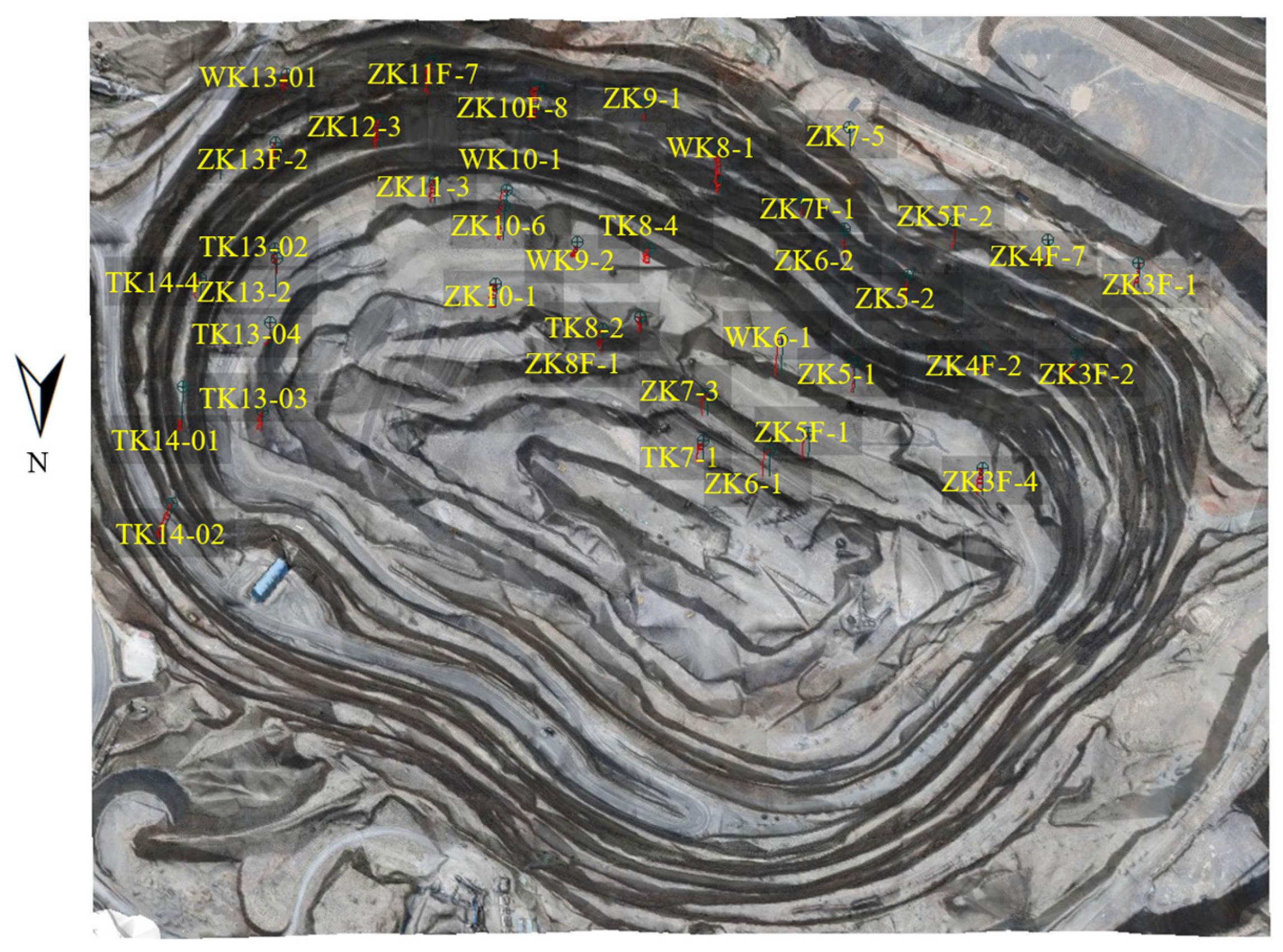
• A spatially variable block model of the rock mass mechanical parameters was developed to support the slope stability assessments. The RQD data were extracted from 40 borehole cores using digital image processing techniques. The three-dimensional spatial interpolation for the unsampled regions employed a spherical semivariogram model (nugget effect = 60; sill = 420; range = 230 m), establishing an RQD block model. The geological parameters were subsequently transformed into mechanical parameters via the generalized Hoek–Brown criterion, enabling the spatial visualization of the rock mass’s mechanical properties.
• The model’s credibility is supported by the leave-one-out cross-validation, which indicates minimal interpolation bias and spatially unstructured errors. The lithology-grouped regressions reveal an exponential E–GSI relation and a near-linear depth dependence of the equivalent cohesion, which together rationalize the observed increase in stiffness and cohesion with depth.
• Comparative stability analyses of the homogeneous and heterogeneous slope models were conducted using the PSF method. When contrasted against three homogeneous baselines (5th/25th/50th percentiles), the heterogeneous parameterization not only aligns with the mapped 2020 sliding surface but also avoids the underestimation (Fs < 1.0) seen in the 5th percentile case and the overestimation (Fs ≫ 1.0) in the 50th percentile case; the commonly used 25th percentile baseline still overpredicts the stability (Fs ≈ 1.17–1.34). These results indicate that spatial heterogeneity governs both the magnitude and geometry of instability, and that homogeneous benchmarks—regardless of the percentile chosen—are insufficient to reproduce the observed failure. Notably, the stability assessments reveal that the limestone formation within the southern slope represents a critical instability hazard, necessitating prioritized geotechnical monitoring and reinforcement measures.

References

1. Nguyen, T.S.; Keawsawasvong, S.; Phan, T.N.; Tanapalungkorn, W.; Likitlersuang, S. Probabilistic Analysis of Rock Slope Stability Considering the Spatial Variability of Rock Strength Parameters. Int. J. Geomech. 2025, 25, 04025002. [Google Scholar] [CrossRef]
2. Gravanis, E.; Pantelidis, L.; Griffiths, D.V. An analytical solution in probabilistic rock slope stability assessment based on random fields. Int. J. Rock Mech. Min. Sci. 2014, 71, 19–24. [Google Scholar] [CrossRef]
3. Li, J.D.; Gao, Y.; Yang, T.H.; Zhang, P.H.; Zhao, Y.; Deng, W.X.; Liu, H.L.; Liu, F.Y. Integrated simulation and monitoring to analyze failure mechanism of the anti-dip layered slope with soft and hard rock interbedding. Int. J. Min. Sci. Technol. 2023, 33, 1147–1164. [Google Scholar] [CrossRef]
4. Zhang, W.G.; Meng, F.S.; Chen, F.Y.; Liu, H.L. Effects of spatial variability of weak layer and seismic randomness on rock slope stability and reliability analysis. Soil Dyn. Earthq. Eng. 2021, 146, 106735. [Google Scholar] [CrossRef]
5. Li, L.L.; Guan, J.F.; Liu, Z.Y. A random discrete element method for modeling rock heterogeneity. Geomech. Geophys. Geo-Energy Geo-Resour. 2022, 8, 12. [Google Scholar] [CrossRef]
6. Lan, H.X.; Zhang, Y.X.; Macciotta, R.; Li, L.P.; Wu, Y.M.; Bao, H.; Peng, J.B. The role of discontinuities in the susceptibility, development, and runout of rock avalanches: A review. Landslides 2022, 19, 1391–1404. [Google Scholar] [CrossRef]
7. Vick, L.M.; Böhme, M.; Rouyet, L.; Bergh, S.G.; Corner, G.D.; Lauknes, T.R. Structurally controlled rock slope deformation in northern Norway. Landslides 2020, 17, 1745–1776. [Google Scholar] [CrossRef]
8. He, Y.; Li, Z.; Ou, J.L.; Yuan, R. Random Finite-Element Analysis of Slope Considering Strength Anisotropy and Spatial Variability of Soil. Nat. Hazards Rev. 2024, 25, 04024010. [Google Scholar] [CrossRef]
9. Cho, S.E. Effects of spatial variability of soil properties on slope stability. Eng. Geol. 2007, 92, 97–109. [Google Scholar] [CrossRef]
10. Liu, F.Y.; Yang, T.H.; Zhou, J.R.; Deng, W.X.; Yu, Q.L.; Zhang, P.H.; Cheng, G.W. Spatial Variability and Time Decay of Rock Mass Mechanical Parameters: A Landslide Study in the Dagushan Open-Pit Mine. Rock Mech. Rock Eng. 2020, 53, 3031–3053. [Google Scholar] [CrossRef]
11. Onyejekwe, S.; Kang, X.; Ge, L. Evaluation of the scale of fluctuation of geotechnical parameters by autocorrelation function and semivariogram function. Eng. Geol. 2016, 214, 43–49. [Google Scholar] [CrossRef]
12. Eivazy, H.; Esmaieli, K.; Jean, R. Modelling Geomechanical Heterogeneity of Rock Masses Using Direct and Indirect Geostatistical Conditional Simulation Methods. Rock Mech. Rock Eng. 2017, 50, 3175–3195. [Google Scholar] [CrossRef]
13. Chen, K.J.; Jiang, Q.H. Stability and reliability analysis of rock slope based on parameter conditioned random field. Bull. Eng. Geol. Environ. 2024, 83, 306. [Google Scholar] [CrossRef]
14. Pinheiro, M.; Vallejos, J.; Miranda, T.; Emery, X. Geostatistical simulation to map the spatial heterogeneity of geomechanical parameters: A case study with rock mass rating. Eng. Geol. 2016, 205, 93–103. [Google Scholar] [CrossRef]
15. Huang, Y.; Zhao, L.; Li, X.R. Slope-Dynamic Reliability Analysis Considering Spatial Variability of Soil Parameters. Int. J. Geomech. 2020, 20, 04020068. [Google Scholar] [CrossRef]
16. Chen, L.L.; Zhang, W.A.; Paneiro, G.; He, Y.W.; Hong, L. Efficient numerical-simulation-based slope reliability analysis considering spatial variability. Acta Geotech. 2024, 19, 2691–2713. [Google Scholar] [CrossRef]
17. Liu, Z.J.; Liu, Z.X.; Peng, Y.B. Dimension reduction of Karhunen-Loeve expansion for simulation of stochastic processes. J. Sound Vib. 2017, 408, 168–189. [Google Scholar] [CrossRef]
18. Wang, Q.; Ren, X.D.; Li, J. Modeling of unstable creep failure of spatial variable rocks subjected to sustained loading. Comput. Geotech. 2022, 148, 104847. [Google Scholar] [CrossRef]
19. Bozorgpour, M.H.; Binesh, S.M.; Fathipour, H. Stability analysis of the slopes composed of heterogeneous and anisotropic clay. Acta Geotech. 2025, 20, 69–87. [Google Scholar] [CrossRef]
20. Chen, D.F.; Xu, D.P.; Ren, G.F.; Jiang, Q.; Liu, G.F.; Wan, L.P.; Li, N. Simulation of cross-correlated non-Gaussian random fields for layered rock mass mechanical parameters. Comput. Geotech. 2019, 112, 104–119. [Google Scholar] [CrossRef]
21. Zhang, W.G.; Goh, A.T.C. Reliability analysis of geotechnical infrastructures: Introduction. Geosci. Front. 2018, 9, 1595–1596. [Google Scholar] [CrossRef]
22. Liu, W.F.; Leung, Y.F. Spatial variability of saprolitic soil properties and relationship with joint set orientation of parent rock: Insights from cases in Hong. Eng. Geol. 2018, 246, 36–44. [Google Scholar] [CrossRef]
23. Chi, S.C.; Feng, W.Q.; Jia, Y.F.; Zhang, Z.L. Application of the soil parameter random field in the 3D random finite element analysis of Guanyinyan composite dam. Case Stud. Constr. Mater. 2022, 17, e01329. [Google Scholar] [CrossRef]
24. Aminpour, M.; Alaie, R.; Kardani, N.; Moridpour, S.; Nazem, M. Highly efficient reliability analysis of anisotropic heterogeneous slopes: Machine learning-aided Monte Carlo method. Acta Geotech. 2023, 18, 3367–3389. [Google Scholar] [CrossRef]
25. Li, J.D.; Yang, T.H.; Liu, F.Y.; Zhao, Y.; Liu, H.L.; Deng, W.X.; Gao, Y.; Li, H.B. Modeling spatial variability of mechanical parameters of layered rock masses and its application in slope optimization at the open-pit mine. Int. J. Rock Mech. Min. Sci. 2024, 181, 105859. [Google Scholar] [CrossRef]
26. Hoek, E.; Brown, E.T. The Hoek-Brown failure criterion and GSI—2018 edition. J. Rock Mech. Geotech. Eng. 2019, 11, 445–463. [Google Scholar] [CrossRef]
27. Lu, N.; Sener-Kaya, B.; Wayllace, A.; Godt, J.W. Analysis of rainfall-induced slope instability using a field of local factor of safety. Water Resour. Res. 2012, 48, W09524. [Google Scholar] [CrossRef]
28. Nie, W.P.; Shi, C. Study on dynamic stability of large-scale underground cavern group during construction period of hydropower station. Appl. Mech. Mater. 2012, 152–154, 820–825. [Google Scholar] [CrossRef]
29. Loyola, A.C.; Pereira, J.M.; Neto, M.P.C. General Statistics-Based Methodology for the Determination of the Geometrical and Mechanical Representative Elementary Volumes of Fractured Media. Rock Mech. Rock Eng. 2021, 54, 1841–1861. [Google Scholar] [CrossRef]
30. Guo, J.T.; Zhang, Z.R.; Mao, Y.C.; Liu, S.N.; Zhu, W.C.; Yang, T.H. Automatic Extraction of Discontinuity Traces from 3D Rock Mass Point Clouds Considering the Influence of Light Shadows and Color Change. Remote Sens. 2022, 14, 5314. [Google Scholar] [CrossRef]
31. Pan, M.; Jiang, S.H.; Liu, X.; Song, G.Q.; Huang, J.S. Sequential probabilistic back analyses of spatially varying soil parameters and slope reliability prediction under rainfall. Eng. Geol. 2024, 328, 107372. [Google Scholar] [CrossRef]
32. Loáiciga, H.A. Groundwater and earthquakes: Screening analysis for slope stability. Eng. Geol. 2015, 193, 276–287. [Google Scholar] [CrossRef]
33. Huang, M.L.; Sun, D.A.; Wang, C.H.; Keleta, Y. Reliability analysis of unsaturated soil slope stability using spatial random field-based Bayesian method. Landslides 2021, 18, 1177–1189. [Google Scholar] [CrossRef]
34. Yao, W.M.; Li, C.D.; Yan, C.B.; Zhan, H.B. Slope reliability analysis through Bayesian sequential updating integrating limited data from multiple estimation methods. Landslides 2022, 19, 1101–1117. [Google Scholar] [CrossRef]
35. Yao, W.M.; Fan, Y.B.; Li, C.D.; Zhan, H.B.; Zhang, X.; Lv, Y.M.; Du, Z.B. A Bayesian bootstrap-Copula coupled method for slope reliability analysis considering bivariate distribution of shear strength parameters. Landslides 2024, 21, 2557–2567. [Google Scholar] [CrossRef]
36. Pang, R.; Xu, B.; Zhou, Y.; Song, L.F. Seismic time-history response and system reliability analysis of slopes considering uncertainty of multi-parameters and earthquake excitations. Comput. Geotech. 2021, 136, 104245. [Google Scholar] [CrossRef]
37. Liu, S.L.; Wang, L.Q.; Zhang, W.A.; Sun, W.X.; Fu, J.; Xiao, T.; Dai, Z.W. A physics-informed data-driven model for landslide susceptibility assessment in the Three Gorges Reservoir area. Geosci. Front. 2023, 14, 101621. [Google Scholar] [CrossRef]
38. Zhang, W.G.; Wu, C.Z.; Tang, L.B.; Gu, X.; Wang, L. Efficient time-variant reliability analysis of Bazimen landslide in the Three Gorges Reservoir Area using XGBoost and LightGBM algorithms. Gondwana Res. 2023, 123, 41–53. [Google Scholar] [CrossRef]
39. Bai, G.X.; Hou, Y.L.; Wan, B.F.; An, N.; Yan, Y.H.; Tang, Z.; Yan, M.C.; Zhang, Y.H.; Sun, D.Y. Performance Evaluation and Engineering Verification of Machine Learning Based Prediction Models for Slope Stability. Appl. Sci. 2022, 12, 7890. [Google Scholar] [CrossRef]
Figure 1. Schematic diagram of the point safety factor method. The blue, green, and red arrows represent the major principal stress directions σ 1 , σ 2 and σ 3 , respectively. The gray plane denotes the potential failure surface.
Applsci 15 08609 g001
Figure 2. Verification of the PSF method: (a) calculation results using the PSF method ( c = 50   kPa , ϕ = 24 ° ); (b) calculation results using the PSF method ( c = 40   kPa , ϕ = 22 ° ); (c) maximum shear strain ( c = 40   kPa , ϕ = 22 ° ); (d) distribution of the plastic zone ( c = 40   kPa , ϕ = 22 ° ). In subfigure (d), the red area indicates the plastic zone, while the light blue area represents the elastic region.
Applsci 15 08609 g002
Figure 3. General overview of the Bayan Obo mining area: (a) the location of the Bayan Obo open-pit mine. The red star and red dot indicate the locations of Beijing and the Bayan Obo iron mine, respectively; (b) the lithological distribution of the Bayan Obo open-pit mine. The dashed black box marks the boundary of the open-pit area.
Applsci 15 08609 g003
Figure 4. Overview of the south slope of the Bayan Obo open-pit mine: (a) landslide on the south slope (29 August 2020); (b) stereographic projection diagram (lower hemisphere projection).
Applsci 15 08609 g004
Figure 5. Interpretation of high-density electrical method for survey line on the south slope.
Applsci 15 08609 g005
Figure 6. Structural planes fitted from point cloud data.
Applsci 15 08609 g006
Figure 7. Statistics of joint geometric parameters (lower hemisphere projection).
Applsci 15 08609 g007
Figure 8. DFN models with varying scales. Colored arrows indicate the combination of the three joint sets to generate the DFN models on the right.
Applsci 15 08609 g008
Figure 9. Uniaxial compression numerical simulation test.
Applsci 15 08609 g009
Figure 10. Borehole RQD information database. Text labels indicate borehole names.
Applsci 15 08609 g010
Figure 11. Construction and cross-validation of RQD block model: (a) spherical semivariogram model fitting for RQD; (b) RQD block model; (c) leave-one-out cross-validation (LOOCV)—predicted vs. observed; (d) quantile–quantile plot of LOOCV standardized residuals; (e) experimental semivariogram of LOOCV residuals.
Applsci 15 08609 g011
Figure 12. Block model: (a) lithology; (b) GSI; (c) Young’s modulus, E m (GPa); (d) cohesion, c (kPa).
Applsci 15 08609 g012aApplsci 15 08609 g012b
Figure 13. Parametric regression analysis: (a) E m G S I by lithology (log-linear fits); (b) c H by lithology (linear fits). The lithology-based color scheme in (b) corresponds to the same legend as shown in (a).
Applsci 15 08609 g013
Figure 14. Numerical computation of 3D models: (a) heterogeneous model; (b) 5th percentile homogeneous model; (c) 25th percentile homogeneous model; (d) 50th percentile homogeneous model.
Applsci 15 08609 g014
Figure 15. PSF calculation results: (a) heterogeneous model; (b) 5th percentile homogeneous model; (c) 25th percentile homogeneous model; (d) 50th percentile homogeneous model; (e) lithological profile and location of the sliding surface. Profiles 1–6 correspond to six slope cross sections oriented from east to west.
Applsci 15 08609 g015