An Improved Galerkin Framework for Solving Unsteady High-Reynolds Navier–Stokes Equations

Abstract

The numerical simulation of unsteady, high-Reynolds-number incompressible flows governed by the Navier–Stokes (NS) equations presents significant challenges in computational fluid dynamics, primarily concerning numerical stability and computational efficiency. Standard Galerkin finite element methods often suffer from non-physical oscillations in convection-dominated regimes, while the multiscale nature of these flows demands prohibitively high computational resources for uniformly refined meshes. This paper proposes an improved Galerkin framework that synergistically integrates a Variational Multiscale Stabilization (VMS) method with an adaptive mesh refinement (AMR) strategy to overcome these dual challenges. Based on the Ritz–Galerkin formulation with the stable Taylor–Hood ($P_2-P_1$) element, a VMS term is introduced, derived from a generalized $\theta$-scheme. This explicitly constructs a subgrid-scale model to effectively suppress numerical oscillations without introducing excessive artificial diffusion. To enhance computational efficiency, a novel a posteriori error estimator is developed based on dual residuals. This estimator provides the robust and accurate localization of numerical errors by dynamically weighting the momentum and continuity residuals within each element, as well as the flux jumps across element boundaries. This error indicator guides an AMR algorithm that combines longest-edge bisection with local Delaunay re-triangulation, ensuring optimal mesh adaptation to complex flow features such as boundary layers and vortices. Furthermore, the stability of the Taylor–Hood element, essential for stable velocity–pressure coupling, is preserved within this integrated framework. Numerical experiments are presented to verify the effectiveness of the proposed method, demonstrating its ability to achieve stable, high-fidelity solutions on adaptively refined grids with a substantial reduction in computational cost.

1. Introduction

The Navier–Stokes (NS) equations stand as the cornerstone of fluid dynamics, providing a mathematical description for the motion of viscous, incompressible fluids [1]. These equations, derived from the fundamental principles of conservation of mass and momentum, have profound implications across a vast spectrum of scientific and engineering disciplines. Their applications range from aerospace engineering, in the design of aircraft and spacecraft [2], and weather forecasting, where they model atmospheric and oceanic currents [3], to biofluid mechanics, for understanding blood flow in the cardiovascular system [4], and even in the creative industries for realistic visual effects [5]. Despite their ubiquity and fundamental importance, the inherent nonlinearity of the convective term, coupled with the pressure–velocity coupling, makes obtaining analytical solutions possible only in a few highly simplified cases [1,3]. Consequently, the advancement of science and technology has become increasingly reliant on numerical approximations to the NS equations, a field known as computational fluid dynamics (CFD) [2].

Among the various numerical discretization techniques, the finite element method (FEM) has emerged as a powerful and versatile tool for CFD [4,6]. Its strength lies in its ability to handle complex geometries and its solid mathematical foundation, rooted in the Galerkin method [7]. The standard Galerkin FEM seeks an approximate solution within a finite-dimensional function space by enforcing the residual of the governing equation to be orthogonal to the test function space [6]. For Stokes flow or low Reynolds number flows, this approach, when paired with appropriate velocity and pressure approximation spaces like the Taylor–Hood element ($P_2-P_1$) [8], which satisfies the crucial inf-sup (or Ladyzhenskaya–Babuška–Brezzi) condition, provides stable and accurate results [9,10].

However, the landscape changes dramatically when the flow Reynolds number (Re) becomes high as is common in many practical applications such as turbulence and boundary layer separation. In such regimes, the nonlinear convection term dominates the viscous diffusion term, leading to two major, intertwined challenges for numerical simulations. The first is a stability issue: the standard Galerkin method becomes inadequate for convection-dominated problems, often producing spurious, non-physical oscillations that can corrupt the entire solution domain [11,12]. To counteract this, stabilized finite element methods were developed. A pioneering and highly influential approach is the Streamline Upwind Petrov–Galerkin (SUPG) method [13], which introduces an additional term to the weighting function, acting along the streamline to add artificial diffusion only where needed, thus suppressing oscillations without overly compromising accuracy [14]. Building upon these ideas, the Variational Multiscale Stabilization (VMS) method offers a more sophisticated framework [15,16]. While SUPG effectively addresses oscillations by adding artificial diffusion along streamlines, VMS offers a more physically consistent approach by explicitly modeling the effect of unresolved subgrid scales on the resolved scales. This fundamental difference often leads to superior accuracy and less intrusive stabilization, particularly in complex, high-Reynolds-number flows where the interaction between scales is significant. Furthermore, compared to traditional Galerkin methods that often suffer from non-physical oscillations in convection-dominated regimes, the VMS component of the framework ensures the physical fidelity of the solution without excessive artificial diffusion. The core concept of VMS is the decomposition of the solution into large (resolved) scales and small (unresolved) subgrid scales. The effect of the unresolved scales on the resolved scales is then modeled, effectively damping numerical oscillations generated by high Reynolds numbers by explicitly constructing and accounting for subgrid-scale effects [17].

The second major challenge is computational efficiency. High-Reynolds-number flows are inherently multiscale, featuring a wide range of spatial and temporal scales, from large energy-containing eddies down to the smallest dissipative structures at the Kolmogorov scale [18]. Resolving all these scales with a uniformly fine computational grid, a technique known as Direct Numerical Simulation (DNS), is prohibitively expensive and often computationally intractable for practical engineering problems [19]. This necessitates a more intelligent approach to mesh generation. Adaptive mesh refinement (AMR) provides a compelling solution to this problem [20]. Guided by a posteriori error estimators, which measure the local error of the numerical solution, AMR techniques dynamically adjust the mesh resolution, placing smaller elements in regions of high flow complexity (e.g., steep gradients, vortices, and boundary layers) and coarser elements elsewhere [21,22]. This strategy significantly reduces the total number of degrees of freedom and, consequently, the computational cost, while maintaining a high level of accuracy where it is most needed [23].

While both VMS and AMR are powerful techniques in their own right, the existing research has often applied them independently, thereby failing to fully exploit their potential synergistic advantages. For instance, many studies have successfully applied VMS to simulate turbulent flows, but without adaptive meshing, they often require globally fine grids, leading to a significant increase in computational effort that contributes little to the accuracy of the results [24]. Conversely, adaptive methods that lack a proper stabilization treatment, such as the one described by Verfürth (2013) [23], can easily lead to numerical oscillations in convection-dominated scenarios, even on an adapted mesh. The true potential for a breakthrough in efficiency and accuracy lies in their combination: using AMR to focus computational power on the dynamically important regions of the flow, while employing VMS to ensure the stability and correctness of the solution on the resulting anisotropic and non-uniform grids.

While previous works have explored aspects of VMS or AMR independently, or even combined them in a less integrated fashion, the distinct novelty of this paper lies in the deep and self-consistent coupling of these two powerful techniques. Unlike traditional approaches where error estimators might operate on the original Navier–Stokes residuals (as in some standard AMR frameworks), this framework introduces a novel posteriori error estimator specifically formulated based on the dual residuals of the VMS-stabilized large-scale equations. This ensures that the adaptive mesh refinement is directly guided by the quality of the VMS solution itself, including the effects of the subgrid-scale model. This integrated design, where stabilization and adaptation mechanisms work in concert rather than as separate, sequential steps, represents a significant advancement over existing methodologies.

The innovation of this paper lies in the construction of such an enhanced Galerkin framework that deeply couples VMS with an AMR strategy. This synergy is realized through a novel posteriori error estimator specifically designed for the VMS system. Unlike traditional estimators that might act on the original Navier–Stokes residuals, the estimator (as detailed in Section 3.3) is formulated based on the dual residuals of the stabilized large-scale equations. This ensures that the adaptive mesh refinement is directly guided by the quality of the VMS solution itself, including the effects of the subgrid-scale model. This approach creates a truly integrated and self-consistent framework where the stabilization and adaptation mechanisms work in concert, rather than as separate, sequential steps. 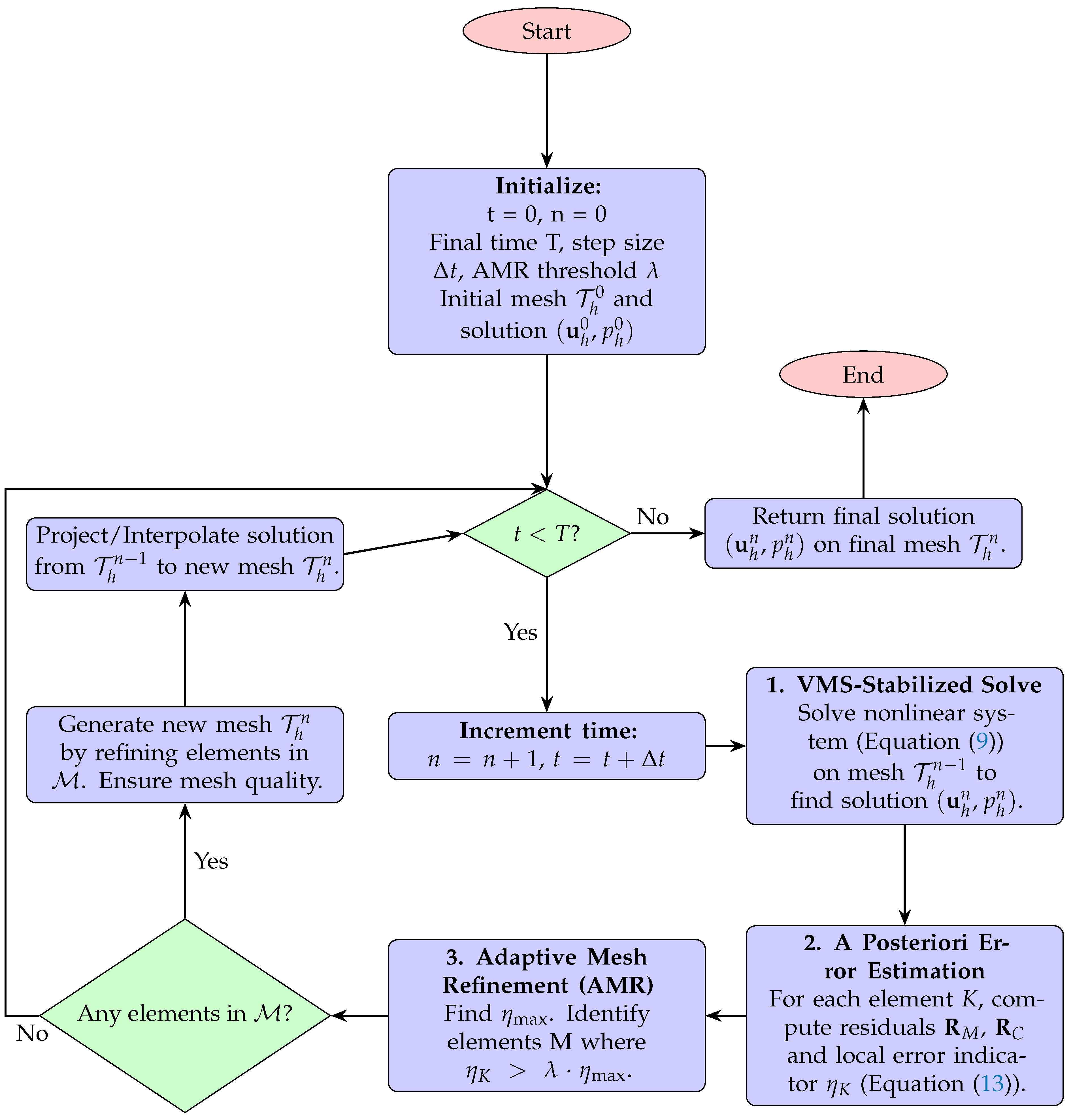Based on the standard Ritz–Galerkin finite element method and the stable Taylor–Hood element, a VMS term is introduced, derived from a generalized $\theta$-scheme for temporal discretization. This explicitly constructs a subgrid-scale model to address the numerical oscillation problem inherent in traditional Galerkin methods for convection-dominated regions. Furthermore, a new posteriori error estimator is designed based on dual residuals, which provides accurate error localization by dynamically weighting local momentum residuals, continuity residuals, and inter-element jump terms. This estimator guides a dynamic mesh refinement strategy, combining the longest-edge bisection method with local Delaunay re-triangulation to ensure mesh quality. The feasibility and superiority of this coupled approach are verified through numerical experiments on high-Reynolds-number flows, demonstrating its capability to provide a robust, accurate, and efficient solution for multiscale problems in computational fluid dynamics.

The remainder of this paper is organized as follows. Section 2 details the mathematical model, presenting the strong and weak forms of the Navier–Stokes equations and discussing the theoretical foundation of the inf-sup condition for mixed finite element methods. In Section 3, the proposed numerical framework is elaborated upon, including the Taylor–Hood element discretization, the formulation of the VMS method, and the design of the posteriori error estimator that drives the adaptive mesh refinement strategy. Section 4.1, Section 4.2, Section 4.3 and Section 4.4 present numerical experiments, focusing on the lid-driven cavity flow benchmark at both high and low Reynolds numbers, to validate the accuracy, stability, and efficiency of the method. Section 4.5 introduces a classical cylinder flow benchmark at Re = 5000 to further demonstrate the framework’s robustness in handling complex, non-steady flows. Finally, Section 5 concludes the paper with a summary of the findings and the key contributions of this work.

2. Mathematical Model

In a bounded convex polygonal region $\Omega$ in ${\mathbb{R}}^n$ (n = 2 or 3) with Lipschitz continuous boundary $\partial \Omega$, the well-known unsteady incompressible NS equations [25] are formulated by

$$\begin{array}{c}\hfill \left\{\begin{array}{cc}\hfill & {\displaystyle \frac{\partial \mathbf{u}}{\partial t}}+(\mathbf{u}·\nabla )\mathbf{u}-\nu \Delta \mathbf{u}+\nabla p=\mathbf{f},\hfill \\ \hfill & \nabla ·\mathbf{u}=0,\hfill \end{array}\right.\mathrm{in}\Omega \times (0,T],\end{array}$$

(1)

with boundary conditions

$$\mathbf{u}=\mathbf{g}\mathrm{on}\partial \Omega ,$$

and initial conditions

$${\mathbf{u}|}_{t=0}={\mathbf{u}}_0{,p|}_{t=0}=p_0,$$

where $\mathbf{u}$ is the velocity field, p is the pressure, $\nu$ is the kinematic viscosity, $\mathbf{f}$ is the volume force, T is the total time for the calculation, and $\mathbf{g}$ is the distribution function of velocity on the boundary. ${\mathbf{u}}_0$ and $p_0$ are the distribution function of velocity and pressure in the flow field at the initial time. Since non-homogeneous problems for Dirichlet boundaries can be transformed into homogeneous problems for the solution, the case of zero boundary conditions will be considered henceforth [26,27].

Let the velocity test function space and pressure test function space be

$$V=\left\{\mathbf{v}\in H^1{(\Omega )\mid \mathbf{v}|}_{\partial \Omega }=\mathbf{0}\right\},Q=\left\{\mathbf{q}\in L^2{(\Omega )\mid \mathbf{q}|}_{\partial \Omega }=\mathbf{0}\right\}.$$

Following a standard derivation, the weak form of (1) is obtained as

$$\begin{array}{c}\hfill \left\{\begin{array}{cc}\hfill & {\int }_{\Omega }{\displaystyle \frac{\partial \mathbf{u}}{\partial t}}·\mathbf{v}d\Omega +{\int }_{\Omega }(\mathbf{u}·\nabla )\mathbf{u}·\mathbf{v}d\Omega +\nu {\int }_{\Omega }\nabla \mathbf{u}·\nabla \mathbf{v}d\Omega -{\int }_{\Omega }p·\nabla \mathbf{v}d\Omega ={\int }_{\Omega }\mathbf{f}·\mathbf{v}d\Omega ,\hfill \\ \hfill & {\int }_{\Omega }\mathbf{q}·(\nabla ·\mathbf{u})d\Omega =0.\hfill \end{array}\right.\end{array}$$

(2)

To solve this problem in a mixed framework, the mixed finite element space $(V_h,Q_h)$ must satisfy the following inf-sup (Ladyzhenskaya–Babuška–Brezzi (LBB)) condition

$$\begin{array}{c}\hfill \underset{\mathbf{q}\in Q_h}{inf}\underset{\mathbf{v}\in V_h}{sup}{\displaystyle \frac{b(\mathbf{v},\mathbf{q})}{{\parallel \mathbf{v}\parallel }_{V_h}{\parallel \mathbf{q}\parallel }_{Q_h}}}\ge {\beta }_h,\end{array}$$

(3)

to ensure the compatibility of the velocity–pressure spaces and to prevent spurious oscillations or non-uniqueness of the pressure solution, where $b(\mathbf{v},\mathbf{q})={\int }_{\Omega }\mathbf{q}·\nabla \mathbf{v}d\Omega$ and ${\beta }_h$ is a constant independent of the mesh size h.

3. Numerical Methods

3.1. Taylor–Hood Element Discretization

In this paper, the Taylor–Hood element space is considered such that

$${\mathbf{v}}_h\in V_h=\{{\mathbf{v}}_h\in V|{\mathbf{v}}_h{|}_K\in P_2\left(K\right),\forall K\in {\mathcal{T}}_h\},{\mathbf{q}}_h\in Q_h=\{{\mathbf{q}}_h\in Q|{\mathbf{q}}_h{|}_K\in P_1\left(K\right),\forall K\in {\mathcal{T}}_h\},$$

and select two sets of basis functions ${\left\{{\varphi }_i\right\}}_{i=1}^{N_u}$ and ${\left\{{\psi }_i\right\}}_{i=1}^{N_p}$, respectively. Since any element in a finite-dimensional space can be expressed as a linear combination of its basis, the velocity field and pressure field can be approximated as

$${\mathbf{u}}_h=\sum _{i=1}^{N_u}{\mathbf{u}}_i{\varphi }_i\left(\mathbf{x}\right),p_h=\sum _{j=1}^{N_p}{p}_j{\psi }_j\left(\mathbf{x}\right),$$

with the piecewise quadratic basis functions ${\varphi }_i$ and linear basic function ${\psi }_i$.

Substituting these approximations into the weak form (2) and choosing the test functions from the same discrete spaces results in a large, coupled system of nonlinear algebraic equations. This system can be expressed in the following block matrix form as

$$\begin{array}{c}\hfill \left[\begin{array}{cc}\mathbf{A}+\mathbf{C}\left({\mathbf{u}}_h\right)& {\mathbf{B}}^T\\ \mathbf{B}& \mathbf{0}\end{array}\right]\left[\begin{array}{c}\mathbf{u}\\ p\end{array}\right]=\left[\begin{array}{c}\mathbf{F}\\ \mathbf{0}\end{array}\right],\end{array}$$

(4)

Among which are

$${\mathbf{A}}_{ij}=\nu {\int }_{\Omega }\nabla {\varphi }_i·\nabla {\varphi }_{j}d\Omega ,$$

$$\mathbf{C}{\left({\mathbf{u}}_h\right)}_{ij}={\int }_{\Omega }({\mathbf{u}}_h·\nabla {\varphi }_j)·{\varphi }_{i}d\Omega ,$$

$${\mathbf{B}}_{ij}=-{\int }_{\Omega }{\psi }_i·\nabla {\varphi }_{j}d\Omega .$$

For the error analysis of this element (4), the velocity field accuracy is $O\left(h^2\right)$ and the pressure field accuracy is $O\left(h\right)$, with a detailed analysis process found in Arnold et al. (2006) [28].

For the temporal discretization, a generalized $\theta$-scheme is employed. This allows for a unified framework to control the accuracy and stability of the time integration. In this work, it has been focused on the second-order accurate and Crank–Nicolson scheme for its excellent long-term stability properties.

First, consider discretizing the time term using a generalized $\theta$-scheme, rewriting the momentum equation in the weak form (2) as

$$\begin{array}{c}\hfill \left\{\begin{array}{cc}\hfill & {\int }_{\Omega }{\displaystyle \frac{{\mathbf{u}}_h^{n+1}-{\mathbf{u}}_h^n}{\Delta t}}·{\mathbf{v}}_{h}d\Omega +\theta [{\int }_{\Omega }({\mathbf{u}}_h^{n+1}·\nabla ){\mathbf{u}}_h^{n+1}·{\mathbf{v}}_h+\nu \nabla {\mathbf{u}}_h^{n+1}·\nabla {\mathbf{v}}_h-p_h^{n+1}·\nabla {\mathbf{v}}_{h}d\Omega ]+\hfill \\ \hfill & (1-\theta )[{\int }_{\Omega }({\mathbf{u}}_h^n·\nabla ){\mathbf{u}}_h^n·{\mathbf{v}}_h+\nu \nabla {\mathbf{u}}_h^n·\nabla {\mathbf{v}}_h-p_h^n·\nabla {\mathbf{v}}_{h}d\Omega ]={\int }_{\Omega }{\mathbf{f}}^{n+\theta }·{\mathbf{v}}_{h}d\Omega ,\hfill \\ \hfill & {\int }_{\Omega }{\mathbf{q}}_h·\nabla ·(\theta {\mathbf{u}}_h^{n+1}+(1-\theta ){\mathbf{u}}_h^n)=0.\hfill \end{array}\right.\end{array}$$

Combining with (4), the final Galerkin system of equations can be obtained as

$$\begin{array}{cc}\hfill & \left[\begin{array}{cc}{\displaystyle \frac{1}{\Delta t}}\mathbf{M}+\theta (\mathbf{A}+\mathbf{C}\left({\mathbf{u}}_h^{n+1}\right))& \theta {\mathbf{B}}^T\\ \theta \mathbf{B}& \mathbf{0}\end{array}\right]\left[\begin{array}{c}{\mathbf{u}}^{n+1}\\ p^{n+1}\end{array}\right]\hfill \\ \hfill =& \left[\begin{array}{c}{\displaystyle \frac{1}{\Delta t}}\mathbf{M}{\mathbf{u}}^n-(1-\theta )(\mathbf{A}+\mathbf{C}\left({\mathbf{u}}_h^n\right)){\mathbf{u}}^n-(1-\theta ){\mathbf{B}}^T{p}^n+{\mathbf{F}}^{n+\theta }\\ -(1-\theta )\mathbf{B}{\mathbf{u}}^n\end{array}\right],\hfill \end{array}$$

(5)

Among which we have

$${\mathbf{M}}_{ij}={\int }_{\Omega }{\varphi }_i·{\varphi }_{j}d\Omega .$$

When $\theta ={\displaystyle \frac{1}{2}}$, the temporal accuracy is $O(\Delta t^2)$, and otherwise it is $O(\Delta t)$. The choice of the time-step size ($\Delta t$) is crucial for both the accuracy and stability of unsteady simulations. The generalized $\theta$-scheme provides flexibility in this regard: for $\theta$ = 0.5 (Crank–Nicolson), the scheme is second-order accurate in time $O(\Delta t^2)$ and unconditionally stable for linear problems, making it suitable for capturing transient phenomena with good fidelity. For other values of $\theta$, the scheme is first-order accurate ($O(\Delta t)$). In high-Reynolds-number flows, where complex transient features like vortex shedding and boundary layer dynamics are prevalent, a sufficiently small $\Delta t$ is essential to accurately resolve these temporal scales and maintain numerical stability. A larger $\Delta t$ might lead to numerical oscillations or an inaccurate representation of the flow evolution, even with spatial stabilization. Therefore, a careful balance between temporal accuracy requirements, stability constraints, and computational cost must be considered when selecting $\Delta t$, especially in conjunction with adaptive mesh refinement which primarily addresses spatial resolution.

3.2. Variational Multiscale Stabilization

The fundamental idea behind the Variational Multiscale Stabilization (VMS) method is to conceptually partition the solution space into resolved (large-scale) and unresolved (small-scale) components. In the context of FEM, the large scales correspond to the discrete information that can be captured by the computational mesh, while the small scales represent the subgrid phenomena that cannot be resolved. The VMS framework provides a systematic way to model the effect of these unresolved small scales back onto the resolved large scales. Unlike traditional stabilization methods that add artificial diffusion somewhat arbitrarily, VMS derives the stabilization term directly from the underlying equations, leading to a more physically consistent and less intrusive form of stabilization.

Following the VMS derivation, first, the solution has been decomposed into large scale $\left(h\right)$ and small scale ${(}^{\prime })$ [15,16] as

$$\begin{array}{c}\hfill \mathbf{u}={\mathbf{u}}_h+{\mathbf{u}}^{\prime },p=p_h+p^{\prime },\end{array}$$

(6)

where ${\mathbf{u}}_h\in V_h\subset H^1(\Omega ),p_h\in Q_h\subset L^2(\Omega )$ are the large-scale solutions, which are the numerical solutions. And ${\mathbf{u}}^{\prime }\in V_h^{\perp }$ and $p^{\prime }\in Q_h^{\perp }$ are small-scale solutions, regarded as unresolvable parts, and approximated by subgrid-scale models. Small scales are updated according to the following method

$$\begin{array}{c}\hfill {\mathbf{u}}^{\prime n+\theta }={\tau }_{1,t}{\displaystyle \frac{1}{\theta \Delta t}}{\mathbf{u}}^{\prime n}-{\tau }_{1,t}{\Pi }^{\perp }\left(a·\nabla {\mathbf{u}}_h^{n+\theta }+\nabla p_h^{n+1}\right),p^{\prime n+\theta }=-{\tau }_2{\Pi }^{\perp }(\nabla ·{\mathbf{u}}_h^{n+\theta }),\end{array}$$

where

$${\tau }_1={\left[{\left(c_1{\displaystyle \frac{\nu }{h^2}}\right)}^2+{\left(c_2{\displaystyle \frac{\left|a\right|}{h}}\right)}^2\right]}^{-1/2},{\tau }_2={\displaystyle \frac{h^2}{c_1{\tau }_1}},{\tau }_{1,t}={\left({\displaystyle \frac{1}{\theta \Delta t}}+{\displaystyle \frac{1}{{\tau }_1}}\right)}^{-1}$$

are stabilization parameters. ${\Pi }^{\perp }=I-\Pi$ is the orthogonal projection operator and $\Pi$ is the standard $L^2$ projection. Their formulations are based on the work of Codina (2002) [29], and it has been incorporated by local, cell-wise information of the velocity field magnitude $\left|a\right|$, which makes the stabilization more sensitive to the local flow dynamics [24]. Furthermore,

$$a={\mathbf{u}}_h^{n+\theta }+{\mathbf{u}}^{\prime n+\theta },$$

$${\mathbf{u}}^{\prime 0}=\mathbf{0},p^{\prime 0}=0,$$

where $p^{n+\theta }=\theta p^{n+1}+(1-\theta )p^n,{\mathbf{u}}_h^{n+\theta }=\theta {\mathbf{u}}_h^{n+1}+(1-\theta ){\mathbf{u}}_h^n$.

Substituting the decomposed solutions into the weak form (2), and separating the contributions of large and small scales (taking large-scale test functions), one has

$$\begin{array}{c}\hfill \left\{\begin{array}{cc}\hfill & {\int }_{\Omega }{\displaystyle \frac{\partial ({\mathbf{u}}_h+{\mathbf{u}}^{\prime })}{\partial t}}·{\mathbf{v}}_{h}d\Omega +{\int }_{\Omega }(({\mathbf{u}}_h+{\mathbf{u}}^{\prime })·\nabla )({\mathbf{u}}_h+{\mathbf{u}}^{\prime })·{\mathbf{v}}_{h}d\Omega +\nu {\int }_{\Omega }\nabla ({\mathbf{u}}_h+{\mathbf{u}}^{\prime })·\hfill \\ & \nabla {\mathbf{v}}_{h}d\Omega -{\int }_{\Omega }(p_h+p^{\prime })·\nabla {\mathbf{v}}_{h}d\Omega ={\int }_{\Omega }\mathbf{f}·{\mathbf{v}}_{h}d\Omega ,\hfill \\ \hfill & {\int }_{\Omega }{\mathbf{q}}_h·(\nabla ·({\mathbf{u}}_h+{\mathbf{u}}^{\prime }))d\Omega =0.\hfill \end{array}\right.\end{array}$$

(7)

Assuming that the magnitude of the small-scale ${\mathbf{u}}^{\prime }$ is much smaller than the large-scale ${\mathbf{u}}_h$, neglecting higher-order small terms ${\mathbf{u}}^{\prime }·\nabla {\mathbf{u}}^{\prime }$, and retaining the first-order cross terms leads to

$$(({\mathbf{u}}_h+{\mathbf{u}}^{\prime })·\nabla )({\mathbf{u}}_h+{\mathbf{u}}^{\prime })\approx {\mathbf{u}}_h·\nabla {\mathbf{u}}_h+{\mathbf{u}}_h·\nabla {\mathbf{u}}^{\prime }+{\mathbf{u}}^{\prime }·\nabla {\mathbf{u}}_h.$$

Next, using the Green’s formula, neglecting higher-order small terms ${\mathbf{v}}_h·\Delta {\mathbf{u}}^{\prime }$ and substituting the previous equations and (6) into (7) yields the VMS form including the stabilization term

$$\begin{array}{c}\hfill \left\{\begin{array}{cc}\hfill & {\int }_{\Omega }{\displaystyle \frac{\partial {\mathbf{u}}_h}{\partial t}}·{\mathbf{v}}_{h}d\Omega +{\int }_{\Omega }({\mathbf{u}}_h·\nabla {\mathbf{u}}_h)·{\mathbf{v}}_{h}d\Omega +\nu {\int }_{\Omega }\nabla {\mathbf{u}}_h·\nabla {\mathbf{v}}_{h}d\Omega -{\int }_{\Omega }{p}_h\nabla ·{\mathbf{v}}_{h}d\Omega \hfill \\ \hfill & +{\int }_{\Omega }{\displaystyle \frac{\partial {\mathbf{u}}^{\prime }}{\partial t}}·{\mathbf{v}}_{h}d\Omega +{\int }_{\Omega }{\mathbf{u}}^{\prime }·{\mathbf{u}}_h·\nabla {\mathbf{v}}_{h}d\Omega +{\int }_{\Omega }{p}^{\prime }\nabla ·{\mathbf{v}}_{h}d\Omega ={\int }_{\Omega }\mathbf{f}·{\mathbf{v}}_{h}d\Omega ,\hfill \\ \hfill & {\int }_{\Omega }{\mathbf{q}}_h\nabla ·{\mathbf{u}}_{h}d\Omega -{\int }_{\Omega }{\mathbf{u}}^{\prime }·\nabla {\mathbf{q}}_{h}d\Omega =0.\hfill \end{array}\right.\end{array}$$

(8)

If the VMS form (8) is written in matrix form (ignoring higher-order small terms), then the following matrix form is obtained as

$$\begin{array}{cc}\hfill & \left[\begin{array}{cc}{\displaystyle \frac{1}{\Delta t}}\mathbf{M}+\theta (\mathbf{A}+\mathbf{C}\left({\mathbf{u}}_h^{n+1}\right)+{\mathbf{S}}_K)& \theta {\mathbf{B}}^T\\ \theta \mathbf{B}-{\mathbf{S}}_C& \mathbf{0}\end{array}\right]\left[\begin{array}{c}{\mathbf{u}}^{n+1}\\ p^{n+1}\end{array}\right]\hfill \\ \hfill =& \left[\begin{array}{c}{\displaystyle \frac{1}{\Delta t}}\mathbf{M}{\mathbf{u}}^n-(1-\theta )(\mathbf{A}+\mathbf{C}\left({\mathbf{u}}_h^n\right)+{\mathbf{S}}_K){\mathbf{u}}^n-(1-\theta ){\mathbf{B}}^T{p}^n+{\mathbf{F}}^{n+\theta }-{\mathbf{S}}_M-{\mathbf{S}}_P\\ -(1-\theta )\mathbf{B}{\mathbf{u}}^n\end{array}\right],\hfill \end{array}$$

(9)

where

$${\mathbf{S}}_M=({\displaystyle \frac{{\mathbf{u}}^{\prime n+1}-{\mathbf{u}}^{\prime n}}{\Delta t}},{\varphi }_i),$$

$${\mathbf{S}}_K=({\mathbf{u}}^{\prime n+1},{\varphi }_i·\nabla {\varphi }_j),$$

$${\mathbf{S}}_P=(p^{\prime n+1},\nabla {\varphi }_i),$$

$${\mathbf{S}}_C=({\mathbf{u}}^{\prime n+1},\nabla {\psi }_i).$$

Due to the equation contains nonlinear terms, Picard iteration or Newton iteration can be used to solve it.

3.3. Adaptive Mesh Refinement

Let the exact solution be $(\mathbf{u},p)$, and the numerical solution be $({\mathbf{u}}_h,p_h)$. Define the error as

$$\begin{array}{c}\hfill {\mathbf{e}}_{\mathbf{u}}=\mathbf{u}-{\mathbf{u}}_h,{\mathbf{e}}_p=p-p_h,\end{array}$$

(10)

On the element boundary $\partial K$, define the normal derivative and pressure jumps

$$[\nu {\partial }_n{\mathbf{u}}_h-p_h\mathbf{n}]=\nu {\partial }_n{\mathbf{u}}_h{{|}_{\partial K}-p_h\mathbf{n}|}_{\partial K}.$$

Substituting the error (10) into the weak form (2), the error equation [20] can be obtained as

$$a({\mathbf{e}}_{\mathbf{u}},\mathbf{v})+b(\mathbf{v},{\mathbf{e}}_p)+b({\mathbf{e}}_{\mathbf{u}},\mathbf{q})\approx {\int }_K{\mathbf{R}}_M·\mathbf{v}dK+{\int }_K{\mathbf{R}}_C·\mathbf{q}dK+{\int }_{\partial K}[\nu {\partial }_n{\mathbf{u}}_h-p_h\mathbf{n}]·\mathbf{v}dS,$$

among which the terms ${\mathbf{R}}_M$ and ${\mathbf{R}}_C$ represent the element-wise residuals for the momentum and continuity equations, respectively. Physically, ${\mathbf{R}}_M$ measures the local imbalance of momentum for the computed solution (i.e., how well it satisfies the momentum conservation law within each element), while ${\mathbf{R}}_C$ measures the local mass imbalance (i.e., the divergence error). The jump term $[\nu {\partial }_n{\mathbf{u}}_h-p_h\mathbf{n}]·\mathbf{v}$ across element boundaries accounts for the non-conformity of the numerical fluxes between adjacent elements. A large residual or a large jump term indicates a region where the numerical solution is a poor approximation of the true solution, signaling the need for mesh refinement:

$$\begin{array}{cc}\hfill {\mathbf{R}}_M:=& ({\displaystyle \frac{{\mathbf{u}}_h^{n+1}-{\mathbf{u}}_h^n}{\Delta t}}+\theta (({\mathbf{u}}_h^{n+1}·\nabla ){\mathbf{u}}_h^{n+1}-\nu \Delta {\mathbf{u}}_h^{n+1}+\nabla p_h^{n+1})+(1-\theta )(({\mathbf{u}}_h^n·\nabla ){\mathbf{u}}_h^n-\hfill \\ \hfill & \nu \Delta {\mathbf{u}}_h^n)+\nabla p_h^n)-{\mathbf{f}}^{n+\theta }+{\mathbf{S}}_M^{n+\theta },\hfill \end{array}$$

$${\mathbf{R}}_C:=\nabla ·{\mathbf{u}}_h^{n+\theta }+{\mathbf{S}}_C^{n+\theta },$$

$$a(\mathbf{u},\mathbf{v})={\int }_{\Omega }{\displaystyle \frac{\partial \mathbf{u}}{\partial t}}·\mathbf{v}d\Omega +{\int }_{\Omega }\left((\mathbf{u}·\nabla )\mathbf{u}\right)·\mathbf{v}d\Omega +\nu {\int }_{\Omega }\nabla \mathbf{u}·\nabla \mathbf{v}d\Omega ,$$

$$b(\mathbf{u},\mathbf{q})={\int }_{\Omega }\mathbf{q}·\nabla ·\mathbf{u}d\Omega .$$

It is crucial to note that in the integrated framework, the residuals ${\mathbf{R}}_M$ and ${\mathbf{R}}_C$ are defined with respect to the VMS-stabilized equations for the large scales (as implied in (8)), not the original Navier–Stokes equations. This is the cornerstone of the deep coupling between the stabilization and adaptation strategies. The VMS method introduces subgrid-scale models that modify the discrete governing equations. Consequently, a meaningful error estimator must assess the accuracy of the numerical solution $({\mathbf{u}}_h,p_h)$ against this modified system. By doing so, the AMR strategy is directly informed by the performance of VMS, concentrating mesh refinement in regions where the subgrid-scale model is most active or where the stabilized large-scale solution still exhibits significant residuals. This self-consistent approach ensures that computational effort is focused precisely where it is needed to improve the quality of the stabilized solution.

To estimate the error, choose the test functions $\mathbf{v}={\mathbf{e}}_{\mathbf{u}}$ and $\mathbf{q}={\mathbf{e}}_p$, and substitute them into the error equation, there is

$$\begin{array}{c}\hfill \parallel {\mathbf{e}}_{\mathbf{u}}{\parallel }_{H^1}^2+{\parallel {\mathbf{e}}_p\parallel }_{L^2}^2={\int }_{\Omega }{\mathbf{R}}_M·{\mathbf{e}}_{\mathbf{u}}d\Omega +{\int }_{\Omega }{\mathbf{R}}_C{\mathbf{e}}_{p}d\Omega +{\int }_{\partial K}[\nu {\partial }_n{\mathbf{u}}_h-p_h\mathbf{n}]·{\mathbf{e}}_{\mathbf{u}}dS,\end{array}$$

(11)

On each cell K, by the Cauchy–Schwarz inequality, one has

$$\left|{\int }_K{\mathbf{R}}_M·{\mathbf{e}}_{\mathbf{u}}dK\right|\le \parallel {\mathbf{R}}_M{\parallel }_{L^2\left(K\right)}{\parallel {\mathbf{e}}_{\mathbf{u}}\parallel }_{L^2\left(K\right)},$$

$$\left|{\int }_K{\mathbf{R}}_C{\mathbf{e}}_{p}dK\right|\le \parallel {\mathbf{R}}_C{\parallel }_{L^2\left(K\right)}{\parallel {\mathbf{e}}_p\parallel }_{L^2\left(K\right)}.$$

$$\left|{\int }_{\partial K}[\nu {\partial }_n{\mathbf{u}}_h-p_h\mathbf{n}]·{\mathbf{e}}_{\mathbf{u}}dS\right|\le \parallel [\nu {\partial }_n{\mathbf{u}}_h-p_h\mathbf{n}]{\parallel }_{L^2(\partial K)}{\parallel {\mathbf{e}}_{\mathbf{u}}\parallel }_{L^2(\partial K)}.$$

Next, based on the properties of the interpolation operator, the error decomposition is given by

$${\mathbf{e}}_{\mathbf{u}}={\mathbf{e}}_{\mathbf{u}}^I+{\mathbf{e}}_{\mathbf{u}}^h,$$

where the interpolation error is ${\mathbf{e}}_{\mathbf{u}}^I=\mathbf{u}-{\Pi }_h\mathbf{u}$, and the discretization error is ${\mathbf{e}}_{\mathbf{u}}^h={\Pi }_h\mathbf{u}-{\mathbf{u}}_h$.

Then, proceed with the interpolation error estimation. Within element K, a Taylor expansion of $\mathbf{u}$ is performed up to order $k+1$ as

$$\mathbf{u}\left(\mathbf{x}\right)=\sum _{\left|\alpha \right|\le k}{\displaystyle \frac{D^{\alpha }\mathbf{u}\left({\mathbf{x}}_c\right)}{\alpha !}}{(\mathbf{x}-{\mathbf{x}}_c)}^{\alpha }+\sum _{\left|\alpha \right|=k+1}{\displaystyle \frac{D^{\alpha }\mathbf{u}\left(\xi \right)}{\alpha !}}{(\mathbf{x}-{\mathbf{x}}_c)}^{\alpha },$$

where ${\mathbf{x}}_c$ is the cell center, $\xi$ is some intermediate point, and D is the derivative operator. Since ${\Pi }_h\mathbf{u}$ is a polynomial of degree $P_k$, the higher-order terms ($\left|\alpha \right|=k+1$) are truncated; hence

$${\mathbf{e}}_{\mathbf{u}}^I\left(\mathbf{x}\right)=\sum _{\left|\alpha \right|=k+1}{\displaystyle \frac{D^{\alpha }\mathbf{u}\left(\xi \right)}{\alpha !}}{(\mathbf{x}-{\mathbf{x}}_c)}^{\alpha }.$$

Using $|\mathbf{x}-{\mathbf{x}}_c|\le h_K$ and $|D^{k+1}{\mathbf{u}|\le |\mathbf{u}|}_{H^{k+1}\left(K\right)}$, there is

$$\parallel {\mathbf{e}}_{\mathbf{u}}^I{\parallel }_{L^2\left(K\right)}\le C{h}_K^{k+1}{\left|\mathbf{u}\right|}_{H^{k+1}\left(K\right)}.$$

Similarly, the gradient error $\nabla {\mathbf{e}}_{\mathbf{u}}^I$ is given by

$$\parallel \nabla {\mathbf{e}}_{\mathbf{u}}^I{\parallel }_{L^2\left(K\right)}\le C{h}_K^k{\left|\mathbf{u}\right|}_{H^{k+1}\left(K\right)}.$$

Take $h={max}_K\left\{h_K\right\}$, and sum over all cells

$$\parallel {\mathbf{e}}_{\mathbf{u}}^I{\parallel }_{L^2(\Omega )}\le C{h}^{k+1}{\left|\mathbf{u}\right|}_{H^{k+1}(\Omega )},$$

$$\parallel {\mathbf{e}}_{\mathbf{u}}^I{\parallel }_{H^1(\Omega )}\le C{h}^k{\left|\mathbf{u}\right|}_{H^{k+1}(\Omega )}.$$

Therefore, for quasi-uniform meshes ($h_K\approx h$), the interpolation error estimate is obtained as

$$\begin{array}{c}\hfill \parallel {\mathbf{e}}_{\mathbf{u}}^I{\parallel }_{H^1}\le C{h}_K{\parallel \mathbf{u}\parallel }_{H^2},\end{array}$$

(12)

where $h_K$ is the element size. The pressure error $\parallel {\mathbf{e}}_p{\parallel }_{L^2}$ is bounded by

$$\parallel {\mathbf{e}}_p{\parallel }_{L^2}\le {\displaystyle \frac{1}{\beta }}\underset{{\mathbf{v}}_h\in V_h}{sup}{\displaystyle \frac{{\int }_{\Omega }{\mathbf{e}}_p·\nabla {\mathbf{v}}_{h}dx}{\parallel {\mathbf{v}}_h{\parallel }_{H^1}}},$$

where $\beta$ is a constant independent of the mesh size. Substituting (10) into the momentum equation (2) yields

$${\int }_{\Omega }{\mathbf{e}}_p·\nabla {\mathbf{v}}_{h}dx=b(\mathbf{v},{\mathbf{e}}_p)={\int }_{\Omega }{\mathbf{R}}_M·{\mathbf{v}}_{h}d\Omega +{\int }_{\partial \Omega }[\nu {\partial }_n{\mathbf{u}}_h-p_h\mathbf{n}]·{\mathbf{e}}_{\mathbf{u}}dS-a({\mathbf{e}}_{\mathbf{u}},\mathbf{v}).$$

Therefore, it can be obtained that the pressure error $\parallel {\mathbf{e}}_p{\parallel }_{L^2}$ is controlled by the velocity error $\parallel {\mathbf{e}}_{\mathbf{u}}{\parallel }_{H^1}$ as

$$\parallel {\mathbf{e}}_p{\parallel }_{L^2}\le {\displaystyle \frac{1}{\beta }}\underset{{\mathbf{v}}_h\in V_h}{sup}{\displaystyle \frac{\left|a({\mathbf{e}}_{\mathbf{u}},\mathbf{v})-{\int }_{\Omega }{\mathbf{R}}_M·{\mathbf{v}}_{h}d\Omega -{\int }_{\partial \Omega }[\nu {\partial }_n{\mathbf{u}}_h-p_h\mathbf{n}]·{\mathbf{e}}_{\mathbf{u}}dS\right|}{\parallel {\mathbf{v}}_h{\parallel }_{H^1}}}.$$

By substituting the error expression (11) into the error estimation on each element K, based on the estimates of the residual and boundary jump terms, as well as the interpolation error estimate (12), the local energy norm control can be obtained as

$$\parallel {\mathbf{e}}_{\mathbf{u}}{\parallel }_{H^1\left(K\right)}^2+{\parallel {\mathbf{e}}_p\parallel }_{L^2\left(K\right)}^2\le C\left(h_K^2\parallel {\mathbf{R}}_M{\parallel }_{L^2\left(K\right)}^2+h_K\parallel [\nu {\partial }_n{\mathbf{u}}_h-p_h\mathbf{n}]{\parallel }_{L^2(\partial K)}^2+{\parallel {\mathbf{R}}_C\parallel }_{L^2\left(K\right)}^2\right).$$

Summing the local estimates over all cells, there is

$$\parallel {\mathbf{e}}_{\mathbf{u}}{\parallel }_{H^1}^2+{\parallel {\mathbf{e}}_p\parallel }_{L^2}^2\le C\sum _K\left(h_K^2\parallel {\mathbf{R}}_M{\parallel }_{L^2\left(K\right)}^2+h_K\parallel [\nu {\partial }_n{\mathbf{u}}_h-p_h\mathbf{n}]{\parallel }_{L^2(\partial K)}^2+{\parallel {\mathbf{R}}_C\parallel }_{L^2\left(K\right)}^2\right).$$

Using discrete stability conditions (such as the inf-sup condition), global posteriori error estimator can be ultimately obtained as

$$\begin{array}{c}\hfill {\eta }_K^2=h_K^2\parallel {\mathbf{R}}_M{\parallel }_{L^2\left(K\right)}^2+h_K\parallel [\nu {\partial }_n{\mathbf{u}}_h-p_h\mathbf{n}]{\parallel }_{L^2(\partial K)}^2+{\parallel {\mathbf{R}}_C\parallel }_{L^2\left(K\right)}^2,\end{array}$$

(13)

where ${\eta }_K$ is the local error indicator. The specific powers of the mesh size $h_K$ (i.e., $h_K^2$ for the element residual and $h_K$ for the jump term) arise from the scaling arguments in the a posteriori error analysis, ensuring that the estimator ${\eta }_K$ correctly reflects the local contribution to the global error in the energy norm. (Adapted from the dual-weighted residual framework of Carstensen and Funken (2001) [30].)

While the fundamental structure of the posteriori error estimator, which balances element residuals and inter-element flux jumps, adapts principles from well-established frameworks for finite element methods (e.g., the dual-weighted residual framework cited from Carstensen and Funken [30]), its novelty and key contribution in this paper lie in its specific formulation and application within the integrated VMS-AMR system.

Specifically, the estimator ${\eta }_K$ is not applied to the original Navier–Stokes equations. Instead, it is crucially formulated based on the residuals ${\mathbf{R}}_M$ and ${\mathbf{R}}_C$ of the VMS-stabilized large-scale equations, which inherently include the subgrid-scale model terms (${\mathbf{S}}_M^{n+\theta }$ and ${\mathbf{S}}_C^{n+\theta }$). This design choice is pivotal for the synergy of the framework. It creates a self-consistent feedback loop: the adaptive mesh refinement is directly guided by the quality of the stabilized solution itself. Consequently, the mesh is refined not only in regions with high physical gradients (e.g., boundary layers and vortices) but also in areas where the subgrid-scale model is most active or exhibits significant residuals. This ensures that computational resources are precisely allocated to improve the fidelity of the coupled VMS-AMR solution, a more nuanced and targeted approach than applying a standard estimator to an unstabilized formulation.

With the posteriori error estimator (13) in hand, adaptive mesh refinement can been implemented. The following is a dynamic refinement strategy for adaptive meshes:

1.

Calculate ${\eta }_K$ for all cells;

2.

Set a threshold $\lambda \in (0,1)$, and mark the units that satisfy ${\eta }_K>\lambda max{\eta }_K$;

3.

Generate a new mesh using the longest-edge bisection method (Rivara (1984) [31]) or local remeshing (Bank et al. (1983) [32]). (Longest-edge bisection: bisect the longest edge of the element, generating a new node. Local remeshing: generate a finer Delaunay triangulation in the marked region.)

The overall workflow of the proposed integrated VMS-AMR framework is summarized in Figure 1 and Algorithm 1 below. This process illustrates the feedback loop where the solution from the VMS-stabilized system is used to calculate an error estimator, which in turn guides the adaptive mesh refinement for the next time step, ensuring that computational effort is dynamically focused on the most critical regions of the flow.

Algorithm 1 Integrated VMS-AMR framework for unsteady Navier–Stokes equations.

1: Initialize: 2: Set time $t\leftarrow 0$, time step counter $n\leftarrow 0$. 3: Define final time T, time step size $\Delta t$, and AMR threshold $\lambda \in (0,1)$. 4: Generate initial mesh ${\mathcal{T}}_h^0$. 5: Set initial velocity ${\mathbf{u}}_h^0$ and pressure $p_h^0$ on ${\mathcal{T}}_h^0$. 6: while$t<T$do 7:  $n\leftarrow n+1$, $t\leftarrow t+\Delta t$. 8:  (1) Solve the VMS system for $({\mathbf{u}}_h^n,p_h^n)$ on mesh ${\mathcal{T}}_h^{n-1}$ 9:  Solve the nonlinear system (e.g., using Picard or Newton iteration) based on Equation (9) to find the large-scale solution $({\mathbf{u}}_h^n,p_h^n)$. 10:  This involves computing stabilization parameters and subgrid-scale model terms. 11:  (2) The Posteriori Error Estimation 12:  for all element $K\in {\mathcal{T}}_h^{n-1}$ do 13:   Compute momentum residual ${\mathbf{R}}_M$ and continuity residual $R_C$ on K using the solution $({\mathbf{u}}_h^n,p_h^n)$. 14:   Calculate the local error indicator ${\eta }_K$ using Equation (13): 15:   ${\eta }_K\leftarrow h_K^2\parallel {\mathbf{R}}_M{\parallel }_{L^2\left(K\right)}^2+h_K\parallel [\nu {\partial }_n{\mathbf{u}}_h-p_h\mathbf{n}]{\parallel }_{L^2(\partial K)}^2+{\parallel R_C\parallel }_{L^2\left(K\right)}^2$. 16:  end for 17:  (3) Adaptive Mesh Refinement (AMR) 18:  Find the maximum error indicator ${\eta }_{max}\leftarrow {max}_{K\in {\mathcal{T}}_h^{n-1}}{\eta }_K$. 19:  Initialize the set of elements to be refined: $\mathcal{M}\leftarrow \varnothing$. 20:  for all element $K\in {\mathcal{T}}_h^{n-1}$ do 21:   if${\eta }_K>\lambda ·{\eta }_{max}$then 22:    $\mathcal{M}\leftarrow \mathcal{M}\cup \left\{K\right\}$. 23:   end if 24:  end for 25:  Generate a new mesh ${\mathcal{T}}_h^n$ by refining elements in $\mathcal{M}$ (e.g., using longest-edge bisection). 26:  Ensure mesh quality and conformity. 27:  Project/Interpolate the solution $({\mathbf{u}}_h^n,p_h^n)$ from ${\mathcal{T}}_h^{n-1}$ to the new mesh ${\mathcal{T}}_h^n$. 28: end while 29: return Final solution $({\mathbf{u}}_h^n,p_h^n)$ on the final mesh ${\mathcal{T}}_h^n$.

4. Numerical Experiments

4.1. Lid-Driven Cavity Flow (Re = 1)

To first verify the fundamental accuracy and convergence rate of the implementation, a standard example needs to be found. However, in the case of high Reynolds number, the academic community has not found its standard exact solution. Therefore, the exact solution for Re = 1 is provided as

$$\begin{array}{cc}\hfill & u_1(x,y,t)={\displaystyle \frac{1}{10}}(6+4cos\left(4t\right))·16{sin}^2\left(\pi x\right)·y(1-y)(1-2y),\hfill \\ \hfill & u_2(x,y,t)={\displaystyle \frac{1}{10}}(6+4cos\left(4t\right))·(-8\pi )sin\left(2\pi x\right)·{\left(y(1-y)\right)}^2,\hfill \\ \hfill & p(x,y,t)={\displaystyle \frac{1}{10}}(6+4cos\left(4t\right))·sin\left(\pi x\right)cos\left(\pi y\right).\hfill \end{array}$$

The initial and boundary conditions are derived from this exact solution. Figure 2 shows the comparison between the numerical solution and the exact solution at $T=0.03$, while

Table 1. The error of each time step in the case of Re = 1.

Time Step	1	2	3	4	5	6	7	8	9	10
${\displaystyle \frac{\parallel \mathbf{u}-{\mathbf{u}}_h{\parallel }_0}{{\parallel \mathbf{u}\parallel }_0}}$	$0.08\%$	$0.08\%$	$0.08\%$	$0.08\%$	$0.08\%$	$0.08\%$	$0.08\%$	$0.08\%$	$0.08\%$	$0.08\%$
${\displaystyle \frac{\parallel \mathbf{u}-{\mathbf{u}}_h{\parallel }_1}{{\parallel \mathbf{u}\parallel }_1}}$	$0.93\%$	$0.92\%$	$0.93\%$	$0.93\%$	$0.93\%$	$0.93\%$	$0.94\%$	$0.93\%$	$0.94\%$	$0.93\%$
${\displaystyle \frac{\parallel p-p_h{\parallel }_0}{{\parallel p\parallel }_0}}$	$3.70\%$	$1.25\%$	$3.96\%$	$1.41\%$	$4.12\%$	$1.54\%$	$4.24\%$	$1.66\%$	$4.32\%$	$1.76\%$
${\displaystyle \frac{\parallel \mathbf{u}-{\mathbf{u}}_h{\parallel }_1+{\parallel p-p_h\parallel }_0}{{\parallel \mathbf{u}\parallel }_1+{\parallel p\parallel }_0}}$	$1.11\%$	$0.94\%$	$1.13\%$	$0.96\%$	$1.14\%$	$0.97\%$	$1.15\%$	$0.98\%$	$1.16\%$	$0.98\%$

and

Table 2. The result error in the case of Re = 1.

Error Type	$\frac{\parallel \mathit{u}-{\mathit{u}}_{\mathit{h}}{\parallel }_0}{{\parallel \mathit{u}\parallel }_0}$	$\frac{\parallel \mathit{u}-{\mathit{u}}_{\mathit{h}}{\parallel }_1}{{\parallel \mathit{u}\parallel }_1}$	$\frac{\parallel \mathit{p}-{\mathit{p}}_{\mathit{h}}{\parallel }_0}{{\parallel \mathit{p}\parallel }_0}$	$\frac{\parallel \mathit{u}-{\mathit{u}}_{\mathit{h}}{\parallel }_1+{\parallel \mathit{p}-{\mathit{p}}_{\mathit{h}}\parallel }_0}{{\parallel \mathit{u}\parallel }_1+{\parallel \mathit{p}\parallel }_0}$
Error magnitude	$0.0832\%$	$0.9785\%$	$1.7646\%$	$0.9785\%$

provide a quantitative error analysis. The results confirm that the numerical solution accurately matches the analytical solution, and the error magnitudes are consistent with the theoretical convergence rates of the Taylor–Hood element.

The error of each time step is shown in Table 1 below.

The concrete final result error is shown in Table 2 below:

4.2. Validation Case: Lid-Driven Cavity Flow at Re = 1000

After confirming the basic accuracy, the solver’s ability is validated to handle flows at a moderately high Reynolds number against a widely recognized benchmark. The lid-driven cavity flow at Re = 1000 is simulated, and the steady-state results are compared with the classic reference data provided by Ghia et al. [33]. This test is crucial for verifying that the VMS formulation can accurately capture the complex flow physics, such as the location and intensity of the primary and secondary vortices, before assessing the efficiency of the adaptive strategy. The simulation is run on a initial $40\times 40$ grid until the flow reaches a steady state ($T=20.0$).

Figure 3 displays the computed steady-state velocity and pressure fields.

Table 3. The velocity on the horizontal central axis compared with the Ghia benchmark solution.

x	0.0000	0.0625	0.0750	0.1000	0.1500	0.2250	0.2375	0.5000	0.8000	0.8625	0.9000	0.9500	0.9625	0.9750	1.0000
velocity	0.000000	0.294770	0.320392	0.395906	0.394536	0.337253	0.319829	0.025269	−0.287976	−0.436970	−0.575520	−0.462410	−0.346950	−0.217880	0.000000
x (Ghia et al.) [33]	0.000000	0.062500	0.070313	0.093750	0.156250	0.226563	0.234375	0.500000	0.804690	0.859375	0.906250	0.945313	0.953125	0.968750	1.000000
velocity (Ghia et al.) [33]	0.00000	0.27485	0.29012	0.32627	0.37095	0.33075	0.32235	0.02526	−0.31966	−0.42665	−0.51550	−0.39188	−0.33714	−0.21388	0.00000

, Figure 4 and

Table 4. The velocity on the vertical central axis compared with the Ghia benchmark solution.

y	0.0000	0.0500	0.0625	0.1000	0.1750	0.2750	0.4500	0.5000	0.6125	0.7375	0.8500	0.9500	0.9625	0.9750	1.0000
velocity	0.000000	−0.215660	−0.255580	−0.358910	−0.412570	−0.256620	−0.081410	−0.041270	0.047776	0.174235	0.326430	0.486039	0.597135	0.804192	1.000000
y (Ghia et al.) [33]	0.000000	0.054688	0.062500	0.101563	0.171875	0.281250	0.453125	0.500000	0.617188	0.734375	0.851563	0.953125	0.968750	0.976563	1.000000
velocity (Ghia et al.) [33]	0.00000	-0.18109	−0.20196	−0.29730	−0.38289	−0.27805	−0.10624	−0.06080	0.05702	0.18719	0.33304	0.46604	0.57492	0.65928	1.00000

, and Figure 5 compare the velocity profiles along the horizontal and vertical centerlines of the cavity with the benchmark data from Ghia et al. The excellent agreement demonstrates that this method correctly reproduces the established physical features of this challenging flow, providing a solid foundation for the subsequent simulations.

4.3. Unsteady Adaptive Simulation at Re = 1000

Having validated the accuracy and steady-state behavior of the solver, the full capability and efficiency of the integrated VMS-AMR framework are now demonstrated. Consider a square cavity size of $\Omega =[0,1]\times [0,1]$, with the velocity at the top boundary of the region as $\mathbf{u}=(1,0)$, and the remaining parts as $\mathbf{u}=\mathbf{0}$. Take $\nu =0.001$ (i.e., Re = 1000), $\lambda =0.5$, $T=5.0$.

This problem is particularly challenging due to the strong velocity gradients near the moving lid and the formation of a large primary vortex accompanied by smaller secondary vortices in the corners. An effective numerical method must capture these multiscale features accurately without spurious oscillations.

Figure 6 and Figure 7 powerfully illustrate the adaptive strategy in action. Starting from an initial uniform mesh, the AMR algorithm dynamically refines the grid, correctly concentrating elements near the walls where boundary layers form and in regions of high vorticity. This targeted refinement is guided by the posteriori error estimator. Figure 8, Figure 9 and Figure 10 show the final computed flow fields on different initial grids. The velocity streamlines clearly depict the large primary vortex and the developing secondary vortices, consistent with the established results in the literature [33]. The pressure contours are smooth and oscillation-free, with the characteristic low-pressure zone at the vortex core, demonstrating the effectiveness of VMS.

The following Figure 10 shows the operation effect at $T=10.0$.

It can be seen that in theory, a uniform mesh of approximately $129\times 129$ grids [33] would be needed to resolve all scales and converge stably. In contrast, this adaptive method achieves stable convergence using an initial $30\times 30$ grid, which dynamically refines to a final mesh with a number of nodes comparable to a much finer uniform grid only in localized regions. The total degrees of freedom are thus reduced by approximately 90% compared to the $129\times 129$ uniform grid, highlighting the immense computational savings.

This significant reduction in degrees of freedom directly translates to immense computational savings, as the computational effort scales nonlinearly with the mesh size. While the adaptive process introduces overheads such as error estimation and remeshing, these costs are demonstrably outweighed by the benefits of concentrating computational power only where it is most needed, leading to a far more efficient simulation compared to uniformly refined meshes that would be computationally intractable for such complex, multiscale flows.

4.4. High-Reynolds-Number Challenge: Lid-Driven Cavity with a Stationary Cylinder at Re = 5000

To demonstrate the full capability of the integrated framework in a truly challenging scenario, the unsteady flow in a square cavity of size $\Omega =[0,1]\times [0,1]$ containing a stationary cylinder is now considered. The cylinder has a radius of $r=0.15$ and is centered at $(0.5,0.5)$. The top boundary moves with velocity $\mathbf{u}=(1,0)$, while all other external and internal (cylinder surface) boundaries are subject to no-slip conditions. The adaptive mesh refinement strategy ensures high-quality mesh generation, particularly around the curved cylinder boundary as illustrated in Figure 11, to accurately capture the complex flow features in this region. The kinematic viscosity is set to $\nu =0.0002$, corresponding to a high Reynolds number of Re = 5000. This configuration is known to produce a highly complex and chaotic flow field, characterized by the interaction between the large primary vortex induced by the lid and the smaller, high-frequency vortices shed from the cylinder.

Despite the chaotic nature of the flow and the presence of sharp, transient gradients, the pressure and velocity fields shown in Figure 12 remain smooth and free of spurious oscillations, a testament to the effectiveness of VMS. The simulation successfully captures the key physical phenomena, including the deformation of the primary vortex by the offset cylinder and the chaotic shedding of secondary vortices. This complex test case confirms that the integrated approach is robust and efficient, capable of tackling high-Reynolds-number flows with complex geometries and intricate physics, which would be computationally prohibitive with a uniformly refined mesh.

To accurately resolve the flow dynamics around the curved cylinder boundary, a robust mesh generation strategy is employed. The initial mesh is constructed to conform to the geometry, and during the adaptive refinement process, local Delaunay re-triangulation is specifically utilized to maintain mesh quality and adapt to the curved interface. This ensures that elements near the cylinder surface are appropriately refined and well-shaped, preventing numerical artifacts and accurately capturing boundary layer phenomena. A detailed view of the refined mesh in this critical region is presented in Figure 11.

4.5. Classical Cylinder Flow at Re = 5000

To further demonstrate the robustness and versatility of the integrated VMS-AMR framework, results for the classical two-dimensional flow past a circular cylinder at a high Reynolds number of Re = 5000 are presented. The computational domain is a rectangular channel $[-0.5,2.0]\times [-0.5,0.5]$, with the cylinder of radius $r=0.1$ centered at $(0.0,0.0)$. A uniform inflow velocity of $u_{i}n=1.0$ is imposed at the left boundary $(x=-0.5)$, while a zero-pressure condition is applied at the right outflow boundary $(x=2.0)$. No-slip boundary conditions are enforced on the top and bottom walls $(y=-0.5,y=0.5)$ and on the cylinder surface. The adaptive mesh refinement strategy ensures high-quality mesh generation, particularly around the curved cylinder boundary and in the wake region as illustrated in Figure 13, to accurately capture the complex flow features in this region. The kinematic viscosity is set to $\mu =0.00004$ to achieve $Re=5000$ based on the cylinder diameter $(D=0.2)$. This benchmark is notoriously challenging due to the formation of the von Kármán vortex street, which involves complex, non-steady vortex shedding and strong shear layers.

Figure 14 displays the computed velocity, pressure, and vorticity fields at $t=1.5000$. The velocity field clearly shows the development of the von Kármán vortex street in the wake of the cylinder, characterized by the alternating shedding of vortices. The velocity magnitude accelerates around the cylinder shoulders and decelerates in the wake, consistent with the inflow velocity. The pressure field exhibits a high-pressure region at the cylinder’s stagnation point and low-pressure regions at the shoulders and within the vortex cores in the wake. These pressure values are within physically reasonable bounds, indicating a stable and accurate pressure solution. The vorticity field provides the most direct evidence of the vortex shedding, showing distinct alternating positive (red) and negative (blue) vorticity concentrations forming the vortex street. The sharp gradients in vorticity near the cylinder surface and within the shear layers are well-resolved. This successful simulation further validates the capability of the VMS-AMR framework to accurately and stably resolve highly complex, non-steady, high-Reynolds-number flows.

The numerical experiments presented in this section collectively validate the proposed framework from several critical perspectives. The simulation at Re = 1, for which an exact solution is available, provides a quantitative verification of the method’s fundamental accuracy (Section 4.1). The steady-state and unsteady adaptive simulations of the lid-driven cavity flow at Re = 1000 (Section 4.2 and Section 4.3) further demonstrate the robustness of VMS and the efficiency of the AMR strategy in capturing well-defined vortex structures on a standard benchmark. The framework’s full capability is then primarily demonstrated through two highly challenging test cases: the unsteady flow in a cavity with a stationary cylinder at a high Reynolds number of Re = 5000 (Section 4.4), and the classical cylinder flow at Re = 5000 (Section 4.5). In this chaotic regime, the VMS-AMR synergy proved essential. It successfully suppressed numerical oscillations while dynamically concentrating computational effort on the complex interactions between shear layers, boundary layers, and shed vortices. This led to a stable, high-fidelity simulation of a physically intricate problem with significant computational savings, a task that would be exceedingly difficult for conventional methods. Taken together, these comprehensive results provide compelling evidence that this integrated framework is not only stable and efficient for a range of complex flows but also mathematically sound and accurate, making it a reliable and powerful tool for a wide range of CFD applications.

5. Conclusions

In this paper, an improved Galerkin framework is presented, designed to effectively address the persistent challenges of numerical stability and computational efficiency inherent in the simulation of unsteady, high-Reynolds-number Navier–Stokes equations. The work successfully demonstrates that a deep, synergistic coupling of Variational Multiscale Stabilization (VMS) with an adaptive mesh refinement (AMR) strategy provides a robust and powerful solution.

The key contributions of this study are threefold. First, a VMS method is introduced, derived from a generalized $\theta$-scheme, which explicitly constructs a subgrid-scale model to quell the non-physical oscillations that plague standard Galerkin methods in convection-dominated regimes. Unlike methods such as Streamline Upwind Petrov–Galerkin (SUPG) that primarily add artificial diffusion, VMS provides a more physically consistent stabilization by directly accounting for subgrid-scale effects, thereby ensuring the physical fidelity of the solution without excessive smearing. This ensures the physical fidelity of the solution. Second, to tackle the challenge of computational expense, a novel and efficient posteriori error estimator is developed based on dual residuals, which is specifically tailored to the VMS formulation. This estimator assesses the residuals of the large-scale stabilized equations, ensuring that the AMR strategy is directly guided by the accuracy of the VMS solution itself. This creates a feedback loop where the stabilization and mesh refinement work in concert, a key aspect of this synergistic framework. Third, and most crucially, the framework is built upon the Taylor–Hood element, whose stability and satisfaction of the essential inf-sup condition are well-established. This preserves the mathematical rigor of the velocity–pressure coupling, as the AMR strategy incorporates local re-triangulation to maintain the mesh quality necessary for the inf-sup condition to hold on the non-uniform, adaptively generated grids.

The performance and superiority of the proposed method were rigorously validated. After verifying accuracy with an analytical solution at Re = 1, the framework demonstrated its robustness on the benchmark lid-driven cavity flow at Re = 1000. Crucially, its full potential was unleashed on a highly complex case of a lid-driven cavity with an offset cylinder at Re = 5000. Furthermore, the framework’s capability to accurately and stably simulate the classical cylinder flow at Re = 5000, a benchmark known for its complex von Kármán vortex street, further underscores its versatility and robustness. Even in this chaotic regime, this integrated approach maintained stability, captured the intricate multiscale vortex dynamics, and achieved stable convergence on grids that were, on average, significantly coarser than what would be required by traditional methods. This led to a substantial reduction in computational cost, without compromising the physical fidelity of the final solution.

Looking forward, the developed framework serves as a powerful and extensible foundation for future research. Immediate next steps include extending the methodology to three-dimensional (3D) simulations. While the extension to 3D introduces significant challenges, particularly concerning the substantial increase in computational cost and the complexity of mesh generation and management (e.g., efficient 3D Delaunay re-triangulation and load balancing for anisotropic meshes), the fundamental principles of VMS and dual-residual error estimation remain applicable. Addressing these challenges will necessitate advanced parallel computing strategies and optimized data structures to fully leverage the benefits of adaptive refinement in a 3D context. Beyond 3D, the framework can be applied to more complex multiphysics problems, such as fluid–structure interaction or flows with heat transfer. Furthermore, optimizing the implementation for parallel computing architectures could unlock its potential for tackling large-scale industrial and scientific applications. In summary, the integrated VMS-AMR approach presented herein offers a robust, accurate, and highly efficient pathway for the simulation of challenging high-Reynolds-number flows, significantly advancing the capabilities of computational fluid dynamics for both academic research and practical engineering analysis.

References

1. Landau, L.D.; Lifshitz, E.M. Fluid Mechanics: Volume 6; Elsevier: Amsterdam, The Netherlands, 1987; Volume 6. [Google Scholar]
2. Anderson, J.D. Computational Fluid Dynamics: The Basics with Applications; Internationally Renowned Mechanics Books-Photocopy Series; Tsinghua University Press: Beijing, China, 2002. [Google Scholar]
3. Cant, S. S. B. Pope, Turbulent Flows, Cambridge University Press, Cambridge, UK, 2000, 771 pp. Combust. Flame 2001, 125, 1361–1362. [Google Scholar] [CrossRef]
4. Donea, J.; Huerta, A. Finite Element Methods for Flow Problems, 1st ed.; Wiley: New York, NY, USA, 2003. [Google Scholar]
5. Bridson, R. Fluid Simulation for Computer Graphics; Taylor and Francis: New York, NY, USA, 2009. [Google Scholar]
6. Zienkiewicz, O.C. The Finite Element Method: Its Basis and Fundamentals, 6th ed.; World Publishing Corporation: Beijing, China, 2008. [Google Scholar]
7. Clough, R. The Finite Element Method in Plane Stress Analysis. In Proceedings of the ASCE Conference on Electronic Computation, New York, NY, USA, 8–9 September 1960; pp. 345–378. [Google Scholar]
8. Taylor, C.; Hood, P. A numerical solution of the Navier-Stokes equations using the finite element technique. Comput. Fluids 1973, 1, 73–100. [Google Scholar] [CrossRef]
9. Babuška, I. The finite element method with Lagrangian multipliers. Numer. Math. 1973, 20, 179–192. [Google Scholar] [CrossRef]
10. Brezzi, F. On the Existence, Uniqueness and Approximation of Saddle-Point Problems Arising from Lagrangian Multipliers. Revue françAise d Automatique Informatique Recherche opéRationnelle MATHématique 1974, 8, 1–26. [Google Scholar] [CrossRef]
11. Roos, H.G. Robust Numerical Methods for Singularly Perturbed Differential Equations; Springer: Berlin/Heidelberg, Germany, 2008. [Google Scholar]
12. Elman, H.; Silvester, D.; Wathen, A. Finite Elements and Fast Iterative Solvers: With Applications in Incompressible Fluid Dynamics, 2nd ed.; Numerical Mathematics and Scientific Computation; Oxford University Press: Oxford, UK, 2014. [Google Scholar]
13. Brooks, A.N.; Hughes, T.J.R. Streamline upwind/Petrov-Galerkin formulations for convection dominated flows with particular emphasis on the incompressible Navier-Stokes equations. Comput. Methods Appl. Mech. Eng. 1982, 32, 199–259. [Google Scholar] [CrossRef]
14. Hughes, T.J.R.; Franca, L.P.; Mallet, M. A new finite element formulation for computational fluid dynamics: I. Symmetric forms of the compressible Euler and Navier-Stokes equations and the second law of thermodynamics. Comput. Methods Appl. Mech. Eng. 1986, 54, 223–234. [Google Scholar] [CrossRef]
15. Hughes, T.J.; Feijóo, G.R.; Mazzei, L.; Quincy, J.B. The variational multiscale method—a paradigm for computational mechanics. Comput. Methods Appl. Mech. Eng. 1998, 166, 3–24. [Google Scholar] [CrossRef]
16. Codina, R. Stabilization of incompressibility and convection through orthogonal sub-scales in finite element methods. Comput. Methods Appl. Mech. Eng. 2000, 190, 1579–1599. [Google Scholar] [CrossRef]
17. Hughes, T.J.R.; Oberai, A.A.; Mazzei, L. Large eddy simulation of turbulent channel flows by the variational multiscale method. Phys. Fluids (1994) 2001, 13, 1784–1799. [Google Scholar] [CrossRef]
18. Frisch, U.; Donnelly, R.J. Turbulence: The Legacy of A. N. Kolmogorov. Phys. Today 1996, 49, 82–84. [Google Scholar] [CrossRef]
19. Sagaut, P. Large Eddy Simulation for Incompressible Flows: An Introduction, 3rd ed.; Scientific Computation; Springer: Berlin/Heidelberg, Germany, 2006. [Google Scholar]
20. Ainsworth, M.; Oden, J.T. A Posteriori Error Estimation in Finite Element Analysis. Comput. Methods Appl. Mech. Eng. 1997, 142, 1–88. [Google Scholar] [CrossRef]
21. Bubuška, I.; Vogelius, M. Feedback and adaptive finite element solution of one-dimensional boundary value problems. Numer. Math. 1984, 44, 75–102. [Google Scholar] [CrossRef]
22. Dörfler, W. A convergent adaptive algorithm for Poisson’s equation. SIAM J. Numer. Anal. 1996, 33, 1106–1124. [Google Scholar] [CrossRef]
23. Verf"urth, R. A Posteriori Error Estimation Techniques for Finite Element Methods, 1st ed.; Numerical Mathematics and Scientific Computation; Oxford University Press: Oxford, UK, 2013. [Google Scholar]
24. Bazilevs, Y.; Calo, V.; Cottrell, J.; Hughes, T.; Reali, A.; Scovazzi, G. Variational multiscale residual-based turbulence modeling for large eddy simulation of incompressible flows. Comput. Methods Appl. Mech. Eng. 2007, 197, 173–201. [Google Scholar] [CrossRef]
25. Gresho, P.M.; Sani, R.L. Incompressible Flow and The Finite Element Method: Advection-Diffusion and Isothermal Laminar Flow; Wiley: New York, NY, USA, 1998; Volume 1. [Google Scholar]
26. Girault, V.; Raviart, P.A. Finite Element Methods for Navier-Stokes Equations: Theory and Algorithms, 1st ed.; Springer Series in Computational Mathematics; Springer: Berlin/Heidelberg, Germany, 1986; Volume 5. [Google Scholar]
27. John, V. Finite Element Methods for Incompressible Flow Problems, 1st ed.; Springer Series in Computational Mathematics; Springer Nature: Cham, Switzerland, 2016; Volume 51. [Google Scholar]
28. Arnold, D.N.; Falk, R.S.; Winther, R. Defferential Complexes and Stability of Finite Element Methods II: The Elasticity Complex. In Compatible Spatial Discretizations; The IMA Volumes in Mathematics and Its Applications; Springer: New York, NY, USA, 2006; pp. 47–67. [Google Scholar]
29. Codina, R. Stabilized finite element approximation of transient incompressible flows using orthogonal subscales. Comput. Methods Appl. Mech. Eng. 2002, 191, 4295–4321. [Google Scholar] [CrossRef]
30. Carstensen, C.; Funken, S.A. Averaging technique for FE-a posteriori error control in elasticity. Part I: Conforming FEM. Comput. Methods Appl. Mech. Eng. 2001, 190, 2483–2498. [Google Scholar] [CrossRef]
31. Rivara, M.C. Algorithms for refining triangular grids suitable for adaptive and multigrid techniques. Int. J. Numer. Methods Eng. 1984, 20, 745–756. [Google Scholar] [CrossRef]
32. Bank, R.E.; Sherman, A.H.; Weiser, H. Refinement algorithm and data structures for regular local mesh refinement. J. Sci. Comput. 1983, 3–17. [Google Scholar]
33. Ghia, U.; Ghia, K.N.; Shin, C.T. High-Re solutions for incompressible flow using the Navier-Stokes equations and a multigrid method. J. Comput. Phys. 1982, 48, 387–411. [Google Scholar] [CrossRef]
Figure 1. A flowchart of the integrated VMS-AMR framework.
Applsci 15 08606 g001
Figure 2. Results at Re = 1, T = 0.03 ( 20 × 20 grids, initial 10 time steps). (a) Velocity field (exact). (b) Pressure field (exact). (c) Velocity field (FEM). (d) Pressure field (FEM).
Applsci 15 08606 g002
Figure 3. Steady-state results at Re = 1000 (initial 40 × 40 grids). (a) Velocity field. (b) Pressure field.
Applsci 15 08606 g003
Figure 4. The velocity on the horizontal central axis compared with the Ghia benchmark solution.
Applsci 15 08606 g004
Figure 5. The velocity on the vertical central axis compared with the Ghia benchmark solution.
Applsci 15 08606 g005
Figure 6. The adaptively refined mesh effect diagram ( 20 × 20 effect diagram). (a) Initial mesh. (b) t = 2.700 . (c) t = 5.700 . (d) t = 15.000 .
Applsci 15 08606 g006
Figure 7. The adaptively refined mesh effect diagram ( 30 × 30 effect diagram). (a) Initial mesh. (b) t = 2.500 . (c) t = 6.700 . (d) t = 10.000 .
Applsci 15 08606 g007
Figure 8. Results at Re = 1000, T = 5.0 ( 50 × 50 grids, initial 60 time steps). (a) Velocity field. (b) Pressure field.
Applsci 15 08606 g008
Figure 9. Results at Re = 1000, T = 5.0 ( 40 × 40 grids, initial 40 time steps). (a) Velocity field. (b) Pressure field.
Applsci 15 08606 g009
Figure 10. Results at Re = 1000, T = 10.0 ( 30 × 30 grids, initial 40 time steps). (a) Velocity field. (b) Pressure field.
Applsci 15 08606 g010
Figure 11. Zoomed view of the adaptively refined mesh near the stationary cylinder at Re = 5000.
Applsci 15 08606 g011
Figure 12. The numerical results of lid-driven cavity with a stationary cylinder ( T = 1.500 ). (a) Velocity field. (b) Pressure field. (c) Vorticity field.
Applsci 15 08606 g012
Figure 13. Zoomed view of the adaptively refined mesh near the circular cylinder for classical cylinder flow at Re = 5000.
Applsci 15 08606 g013
Figure 14. Numerical results for classical cylinder flow at Re = 5000 ( t = 1.5000 ) . (a) Velocity field. (b) Pressure field. (c) Vorticity field.
Applsci 15 08606 g014