Reducing the Stochastic Coal Output Model Using the Convolution of Probability Density Functions

Abstract

The construction of stochastic models and the use of stochastic simulations for their analysis constitute research methods used in the analysis of stochastic processes. These methods can be applied to processes carried out in underground mines. For mining processes, carried out, e.g., in hard coal mines, it is noticed that the influence of factors generally referred to as geological–mining and technical–organizational may cause a given process to be treated as not fully defined (not necessarily in terms of the process technology, but, e.g., taking into account the time taken for its implementation). This article draws attention to the possibilities of reducing the stochastic model based on the use of the properties of the convolution of probability density functions. Functions that were considered appropriate for describing the processes discussed based on time-based studies were presented. The mechanism of operation of the proposed model reduction was discussed. Reduction carried out in this way eliminates the need to analyze these parts of the model, e.g., using the stochastic simulation method. This reduction leads to simplification of the model and the calculations, which translates into the effectiveness of the research.

1. Introduction

The methods for analyzing a technological process carried out in the longwall face of a hard coal mine take into account the specific geological–mining and technical–organizational conditions of this process. The coal’s workability, the type of roof, the type of floor, the efficiency of the machines used to create a longwall face, and complex mechanization systems dictate the choice of technology and the organization of the exploitation works carried out in the longwall face. However, changing geological–mining conditions—along with the advancement of the longwall face—make it necessary to analyze the impact of these changes on the course of the process, as well as the extraction achieved.

The exploitation of hard coal in Polish deep mines is determined by factors that make it a stochastic process. These factors can be divided into two groups: mining–geological conditions and technical–organizational conditions.

Mining–geological conditions include

-

The type of roof;

-

The type of floor;

-

The workability of the coal;

-

The thickness and slope of the seam;

-

Natural hazards.

Technical and organizational conditions which have a significant impact on the course of the production process include

-

The mechanization system;

-

The technical parameters of the shearer/support parameters;

-

The stochastic failure rate;

-

The organization of the production cycle, which consists of the form of organization of the work and the system of work;

-

The training and experience of employees.

In order to analyze technological processes conditioned in this way, stochastic models of these processes are created and analyzed, in the description of which random variables are used.

The beginning of using methods to analyze stochastic processes in mining dates back to the 1970s. M. Kozdrój, in his work [1], emphasized the importance of probability theory and mathematical statistic methods for the organization of mining production. It is worth noting that this was the first work in which attention was drawn to the wide possibilities of using probability theory for the issues discussed. However, it is worth noting that geological–mining conditions have either remained the same since the 1970s or become worse for coal mining. Exploitation is occurring at an increasing depth, making the conditions more difficult and less predictable, which introduces greater probability into today’s exploitation [2].

In the work [3], J. Antoniak and A. Wianecki proposed the use of simulation methods to study stochastic processes in mining technology. Network methods were also introduced for mining considerations [4]. The work [4] models mining processes in extremely difficult conditions using fuzzy set elements. New research possibilities appeared with the introduction of computing machines and the development of information systems. Progress was made in the construction of numerical models of mining processes conducted in the longwall faces of hard coal mines.

In 1986, W. Kozioł published an article [5] in which he revealed the rhythmicity of the mining process and some of its causes in opencast lignite mining, using a spectral analysis of stochastic processes.

In [6], the reliability of a hydraulic excavator system was analyzed using a non-uniform Poisson process with time-dependent log–linear hazard coefficient functions and a failure mode and effect analysis. Analytical, numerical, and empirical tools were also used to improve the work planning and efficiency [7].

In [8], the evaluation strategies and statistical methods for generating the stochastic fracture networks used for quantitative risk assessments of underground industrial waste storage in hard coal mines using numerical models were summarized. In [9], the influence of advanced technical problems on the efficiency of selected mines was investigated. In [10], stochastic methods for analyzing the production process carried out in longwall faces were presented.

Analytical modeling is also used for issues related to natural hazards [11,12], the optimization of technological flows [13,14,15,16,17], extraction volume [18], mine planning [19,20,21], and even in the design of computer systems used to improve the efficiency of mine rescue systems. Random variables that occur in stochastic models may be subject to probabilistic relationships. One of the most common probabilistic relationships for random variables is their sum (e.g., the total process time as the sum of its individual fragments, the total employment as the sum of staff, the daily output from a longwall face as the sum of the extraction obtained in individual work shifts, etc.). In the conducted studies [22,23], the usefulness of this type of models was noted.

Therefore, in the subsequent part of this paper, the authors put forward the hypothesis that it is possible to use the properties of the convolution of a random variable function to reduce the stochastic model, in particular to model the processes carried out in the longwall faces of hard coal mines.

Recent decades have seen growing interest in the use of stochastic approaches in various areas of mining engineering. Brzychczy [13] proposed probabilistic models tailored to the production systems in underground coal mines, highlighting the necessity of incorporating real-time variability into system modeling. Chen et al. [14] introduced stochastic Petri nets to model disaster chains triggered by mining subsidence, demonstrating the flexibility of stochastic structures in representing complex interdependencies.

Additional research has focused on optimization of the technological flows and production scheduling under uncertain conditions. For example, Khorolskyi et al. [15] and Soleimanfar et al. [16] showed how geological and operational uncertainties affect production efficiency and reliability, integrating stochastic parameters into the optimization algorithms. This approach also appears in studies that apply Monte Carlo simulations to rockburst predictions [11] and stochastic fracture networks to risk modeling in waste repositories [8].

Beyond process-level modeling, stochastic methods have also been used in mine planning and risk assessments. Galetakis et al. [20] incorporated the uncertainty in coal quality and reserves into mine scheduling, while Pavlovic et al. [21] applied stochastic tools to assessing the social and environmental risks in surface mining.

Particularly notable is the application of stochastic modeling to time-based production analyses—such as shift-wise or daily output modeling—where convolution of probability density functions offers a practical way to model the cumulative variability. Snopkowski et al. [22,23] emphasized how process fragments (e.g., the time durations of sub-activities) can be modeled as random variables and their summation described analytically via convolution. This approach avoids unnecessary simulations while preserving the model’s fidelity and transparency.

This modeling strategy aligns with the central limit theorem, which justifies the approximation of sums of independent random variables using normal distributions under certain assumptions. Depending on the process characteristics, other distributions—such as chi-square and gamma—are also frequently used to reflect specific empirical observations better [24,25].

These developments confirm that accounting for stochastic dependencies is indispensable in modern mining research. This paper contributes to the field by proposing a method for stochastic model reduction using the convolution properties of probability density functions, with particular attention to longwall mining operations. This simplification enhances both the analytical clarity and practical applicability of the models in mining practice.

2. Materials and Methods

The probability density functions presented in this section are used to model the mining production process; hence, their properties are presented.

The probability density functions proposed by the authors may constitute probabilistic models of the production cycle. The following criteria for selecting these functions were adopted: the domain of the function should be a set of real positive values or a subset thereof; the function should be unimodal.

For a continuous probability density function $f\left(x\right),$ these properties are as follows [24]:

• The probability density values are greater than or equal to zero:

  $$f\left(x\right)\ge 0$$

  (1)
• The probability of a random variable taking the value $a$ from the interval $(a, b)$ is equal to the definite integral of the function on the interval from $a$ to $b$:

  $$P\left(a\le X\le b\right)=\underset{a}{\overset{b}{\int }}f\left(x\right)dx$$

  (2)
• The integral of the probability density in the range from minus to plus infinity is equal to $1$:

  $$\underset{-\infty }{\overset{\infty }{\int }}f\left(x\right)dx=1$$

  (3)
• At points where $f\left(x\right)$ is continuous, this relationship holds:

  $$f\left(x\right)=F^{\prime }\left(x\right)$$

  (4)

  where $F\left(x\right)$ is the distribution function of the random variable $x$.

Various probability density functions can be used to describe the subsequent activities required by the process or, more precisely, the duration of these activities. This results in obtaining information regarding the level of the coal output. The most commonly used are the following:

2.1. The Chi-Square Distribution

The chi-square distribution with $n$ degrees of freedom is the distribution of a random variable that is the sum of $n$ independent random variables with a standard normal distribution

$$Y_n=\sum _{i=1}^n{X_i}^2$$

(5)

where $X_i$ has a distribution of $N\left(\mathrm{0,1}\right)$.

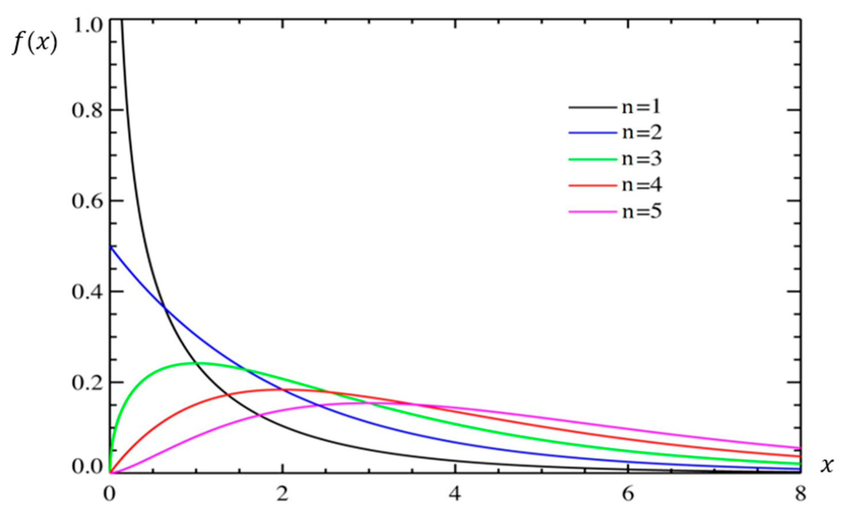
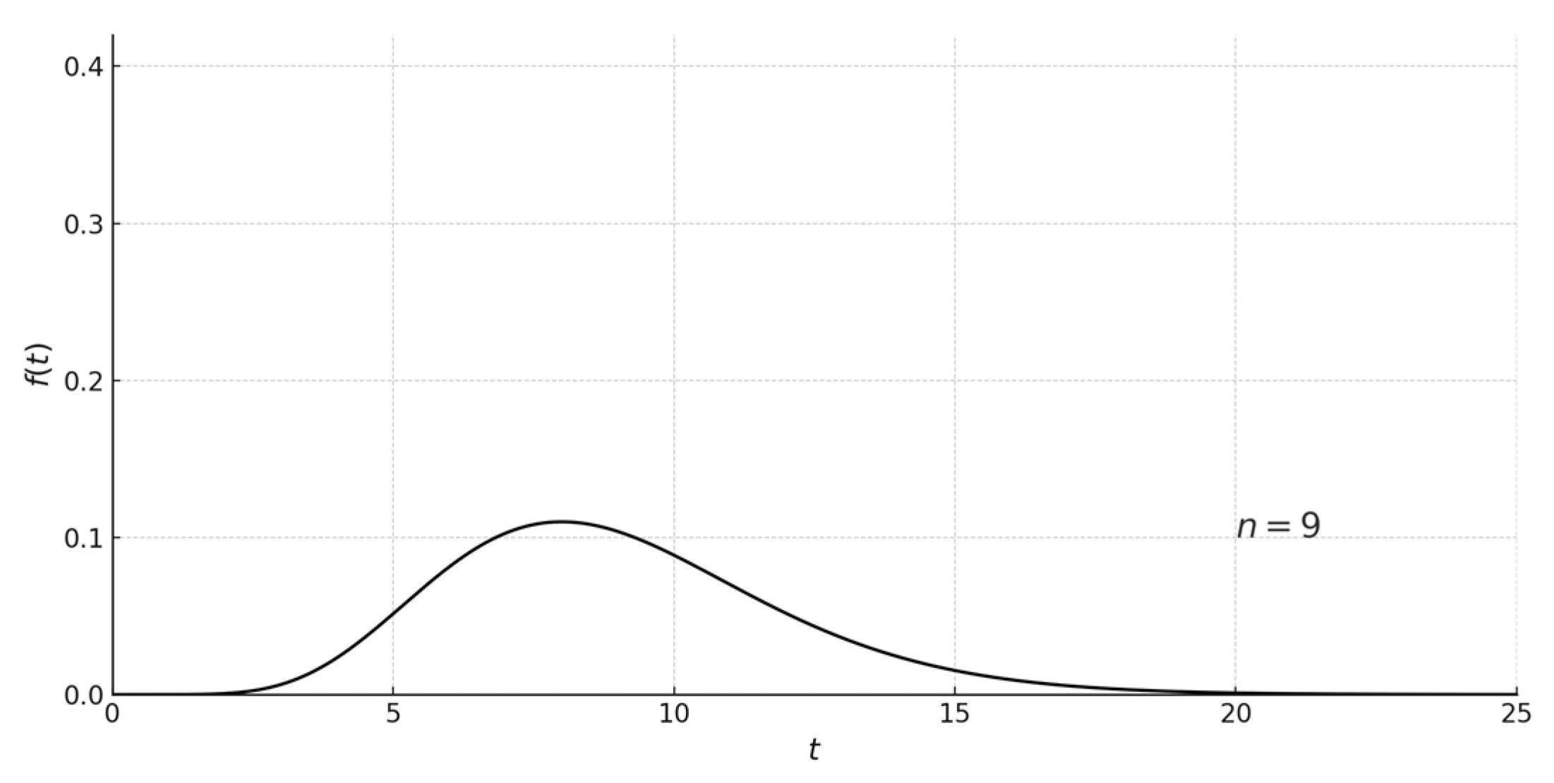
The probability density (Figure 1) of a random variable with a distribution of Chi-square is expressed using the formula

$$f\left(y\right)=\left\{\begin{array}{c}0 dla y\le 0\\ {\displaystyle \frac{1}{2^{\frac{n}{2}}\Gamma \left(\frac{n}{2}\right)}}{y}^{{\displaystyle \frac{n}{2}}-1}{e}^{-{\displaystyle \frac{y}{2}}} dla y>0\end{array}\right.$$

(6)

If $n\le 2$, then, the probability density is a decreasing function for $y>0$, while for $n>2,$ it has a single maximum at point $n-2$. Figure 1 and Figure 2 present graphs of the probability density and the distribution function of a random variable with a chi-square distribution for $n=\mathrm{1,2},\dots ,5$.

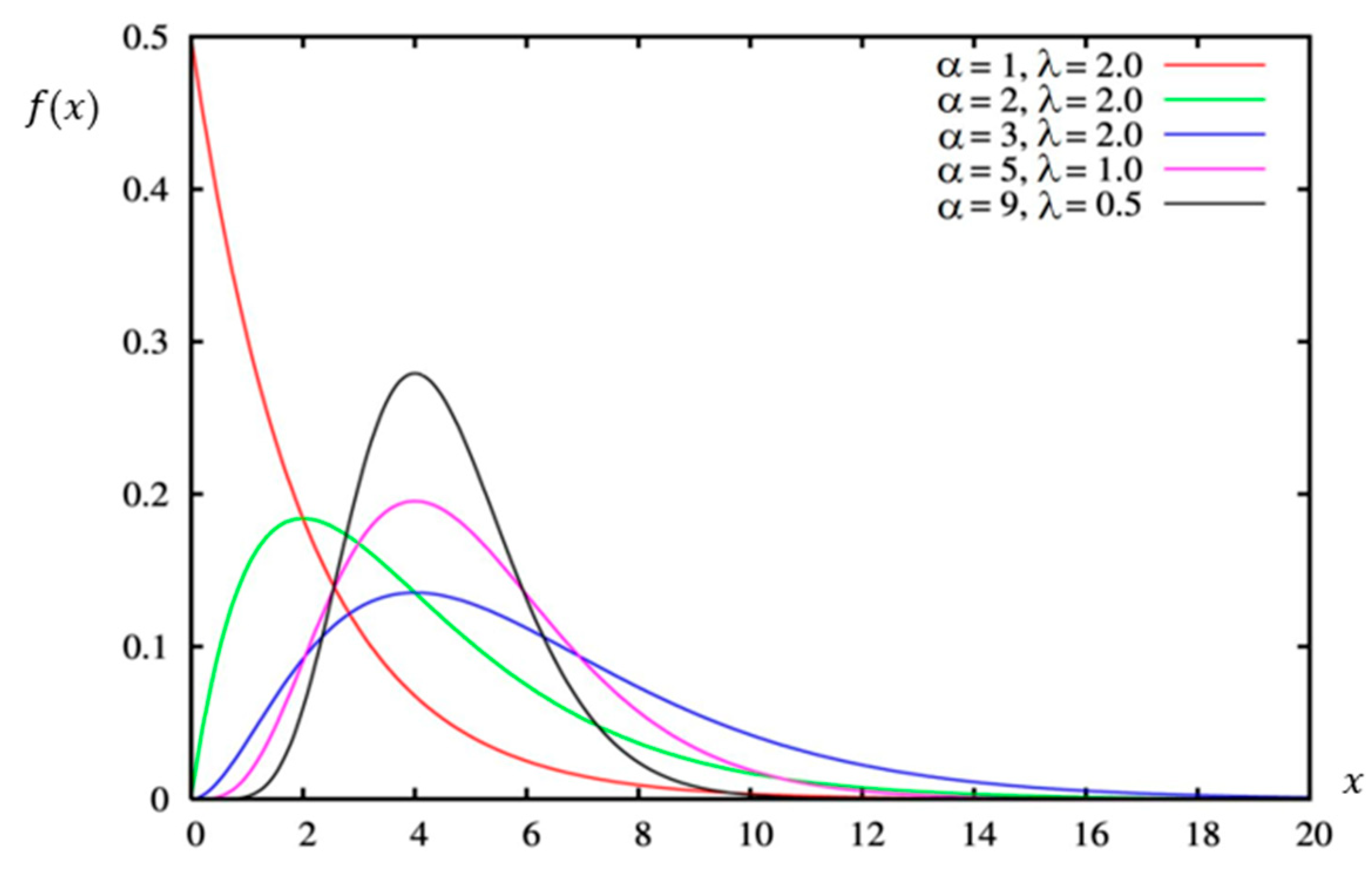
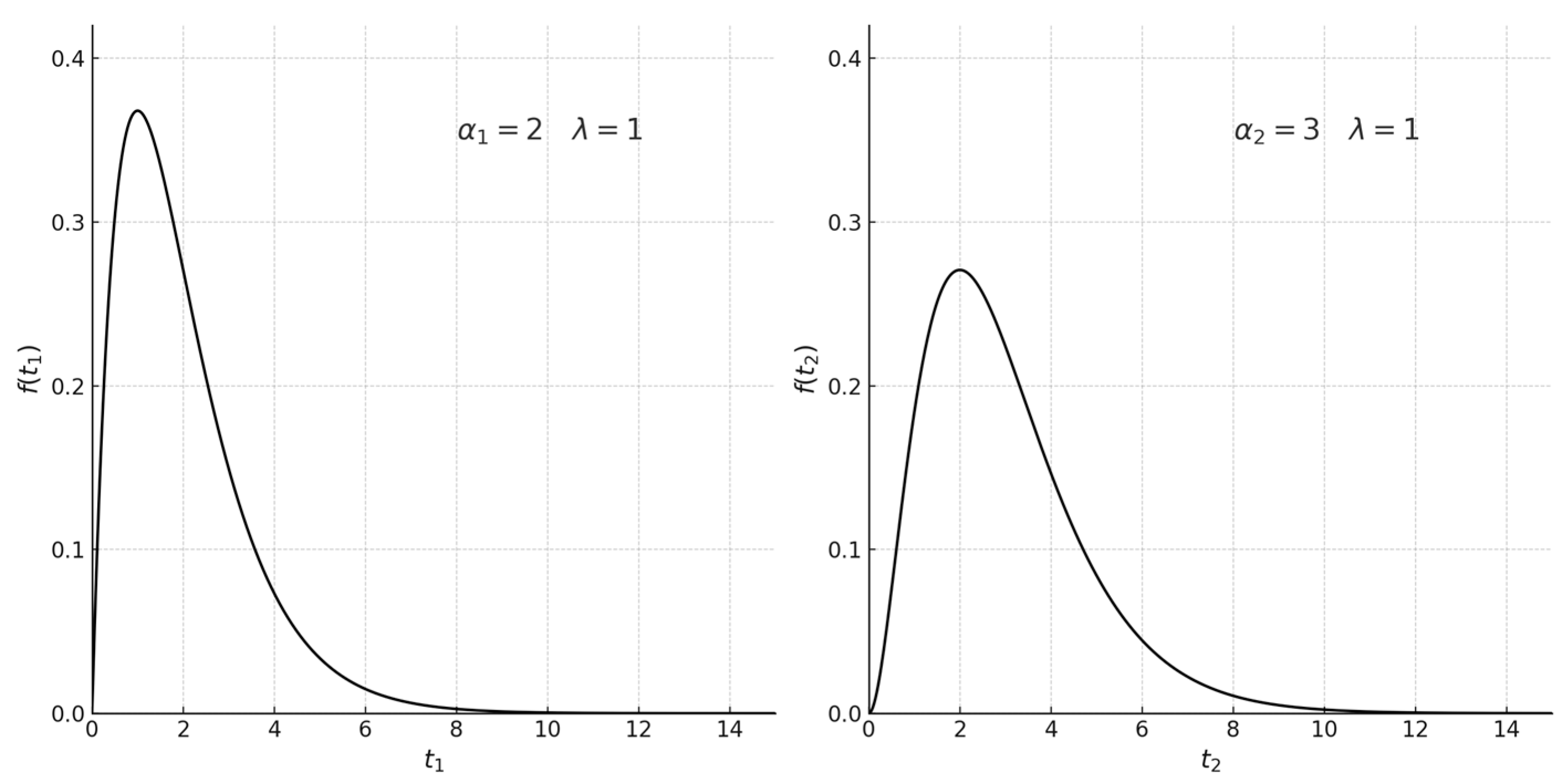
2.2. The Gamma Distribution

The random variable $X$ has a gamma distribution with the parameters $\alpha$ and $\lambda$ when its density is given by the formula

$$f\left(x\right)=\left\{\begin{array}{cc}0& dla x\le 0 \\ {\displaystyle \frac{{\lambda }^{\alpha }}{\Gamma \left(\alpha \right)}}{x}^{\alpha -1}{e}^{-\lambda x}& dla x>0, \left(\alpha >0, \lambda >0\right)\end{array}\right.$$

(7)

where $\Gamma \left(\alpha \right)$ is the gamma function, which is defined by the formula

$$\Gamma \left(\alpha \right)=\underset{0}{\overset{\infty }{\int }}{x}^{\alpha -1}{e}^{-x}dx, \left(\alpha >0\right)$$

(8)

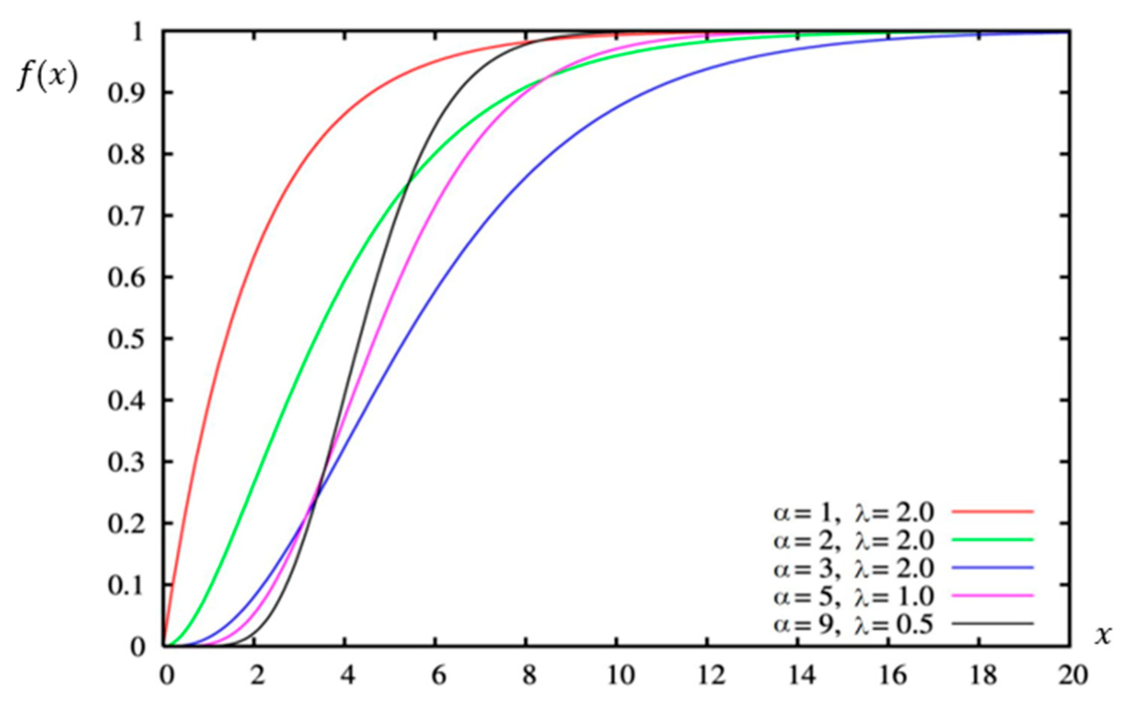
Figure 3 and Figure 4 show examples of probability density functions and distribution functions of the gamma distribution.

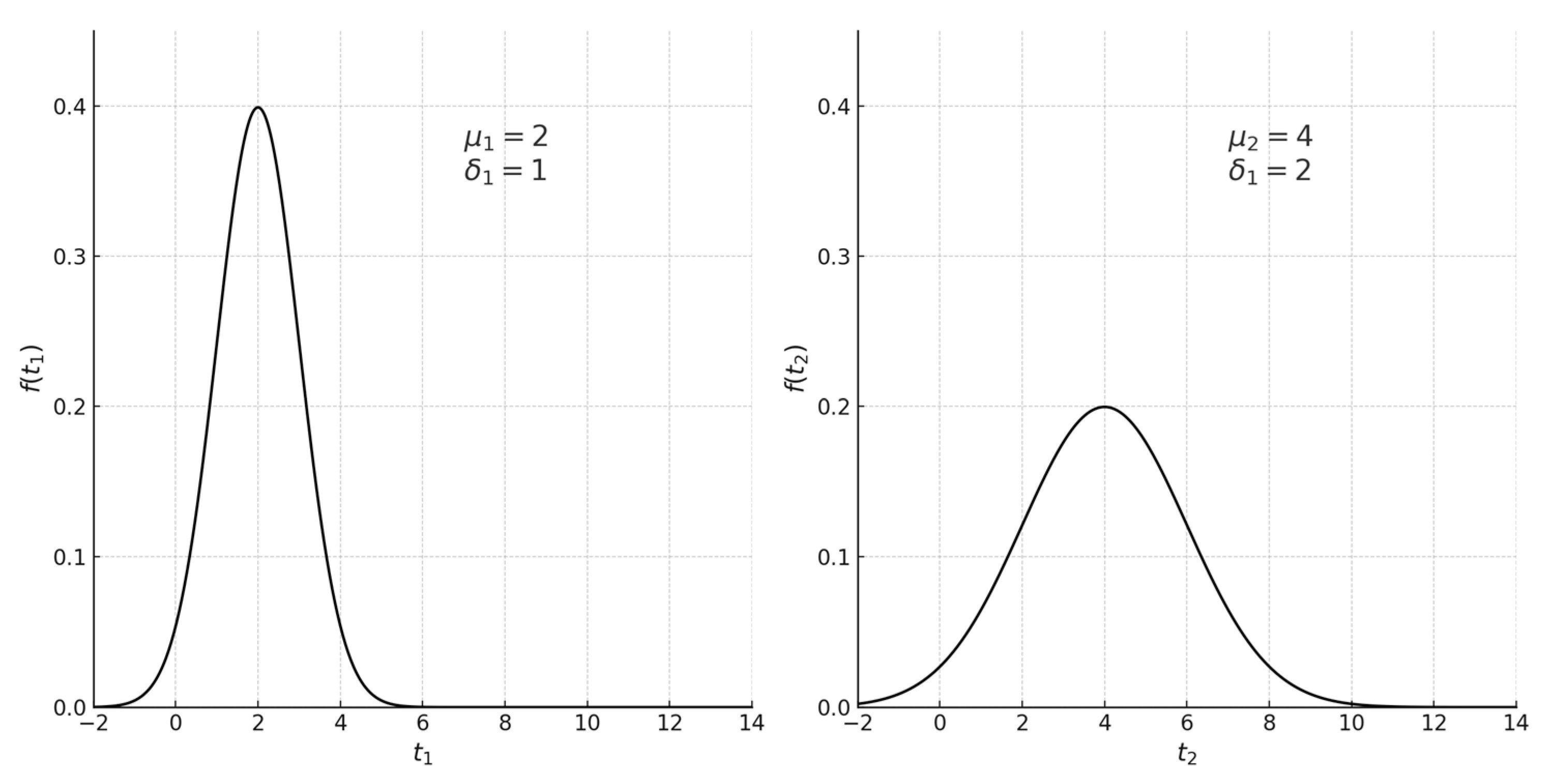
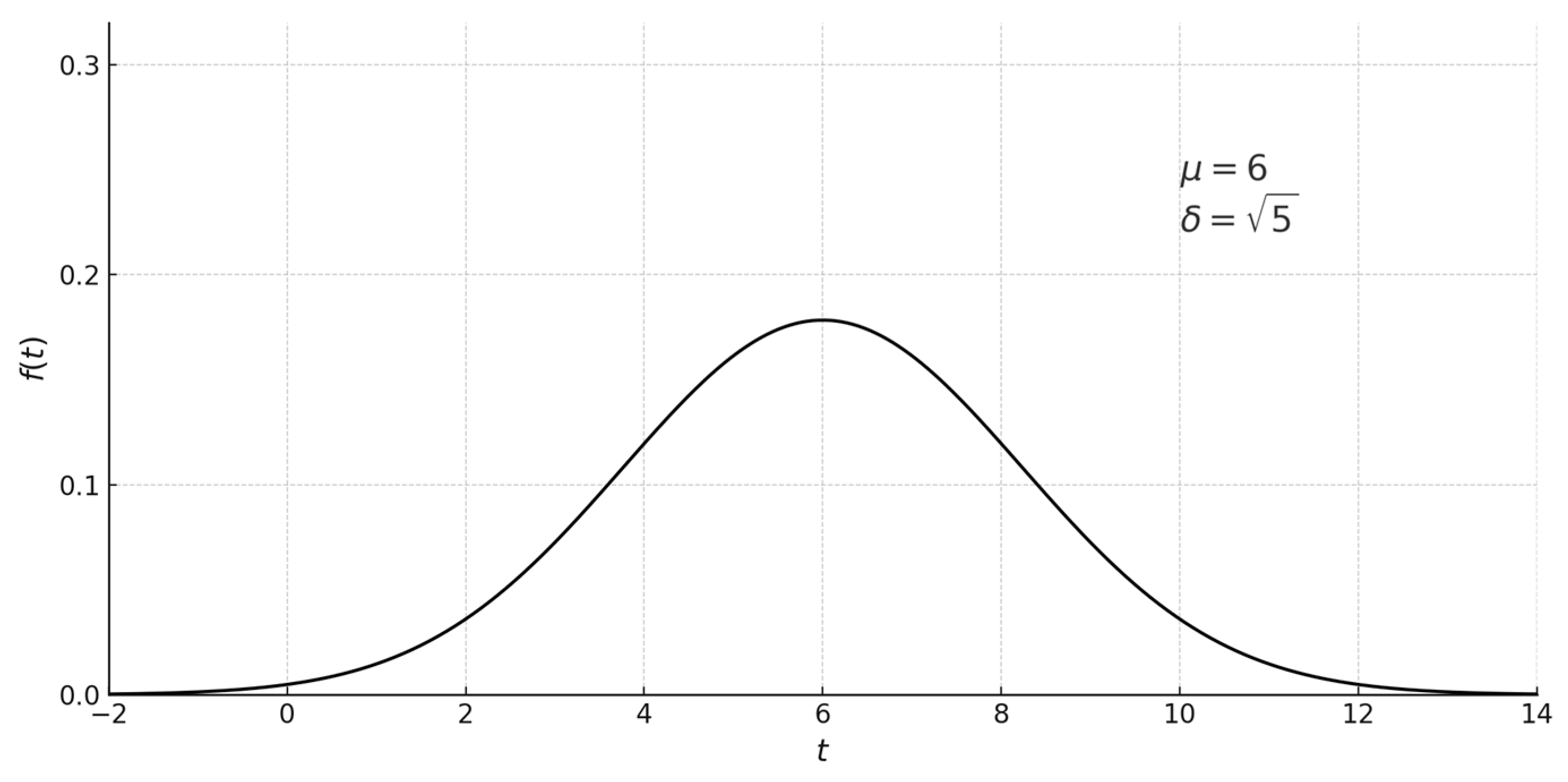
2.3. The Normal Distribution

A continuous random variable $X$ has a normal distribution $N(\mu ,\sigma )$ if its density is given by the formula

$$f\left(x\right)={\displaystyle \frac{1}{\sqrt{2\pi }\sigma }}{e}^{-{\displaystyle \frac{{(x-\mu )}^2}{2{\sigma }^2}}}, (\sigma >0)$$

(9)

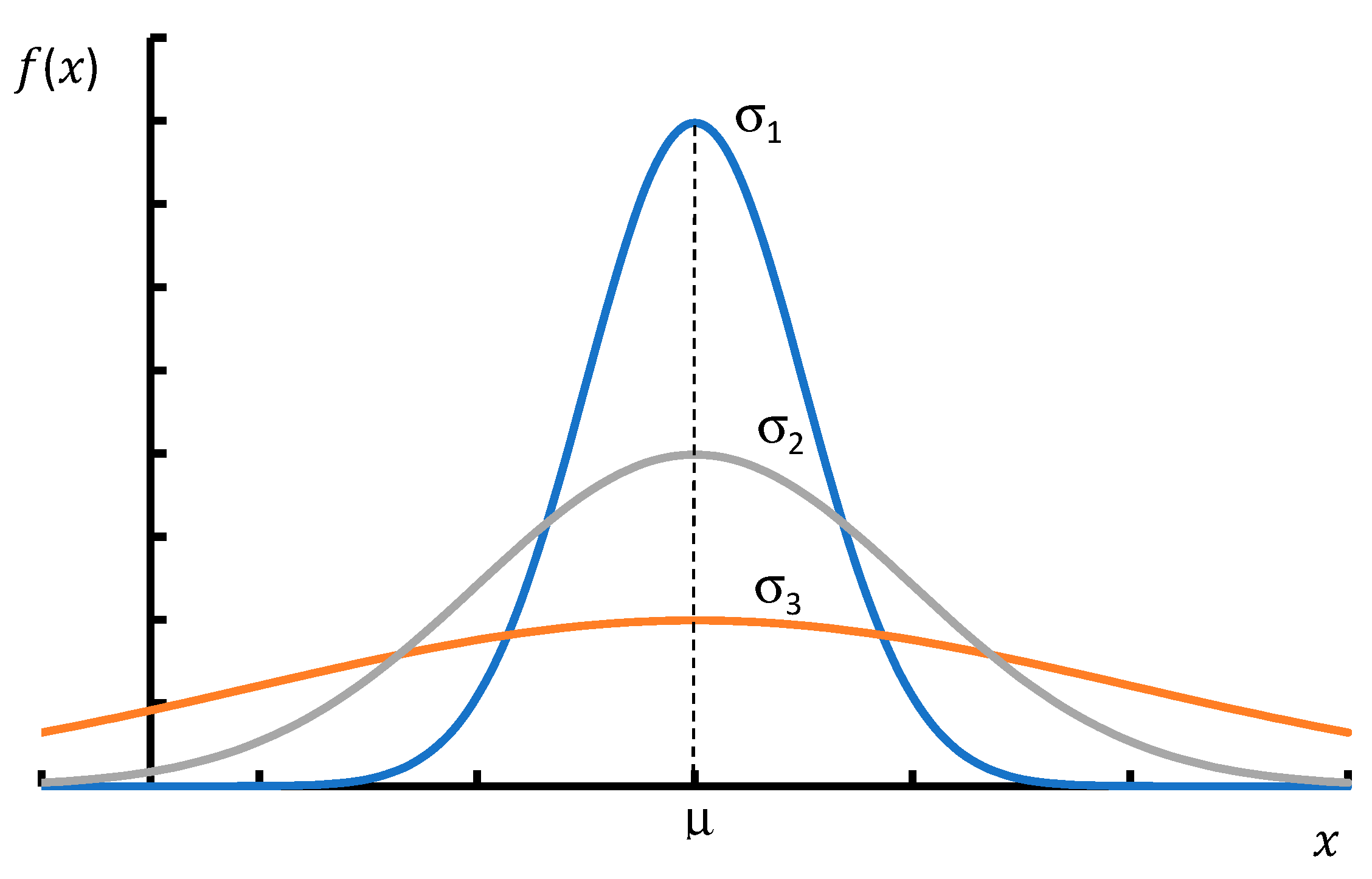
The parameter $\mu$ is the expected value of the random variable $X$, and $\sigma$ is the standard deviation of this variable. Figure 5 presents density plots of three random variables with a normal distribution, where the expected value is the same for all variables, and the standard deviations are ${\sigma }_1<{\sigma }_2<{\sigma }_3$, respectively. It is clearly visible that the smaller the standard deviation σ, the more the distribution is concentrated around the expected value. This is consistent with the previously given interpretation of the parameter $\sigma$.

The inflection point of the curve is one standard deviation away from the expected value. A random variable $Y$ with a normal distribution $N\left(\mathrm{0,1}\right)$ has a density of

$$f\left(x\right)={\displaystyle \frac{1}{\sqrt{2\pi }}}{e}^{-{\displaystyle \frac{x^2}{2}}}$$

(10)

This variable is obtained from a normally distributed random variable $N(\mu ,\sigma )$ through the following transformation:

$$Y={\displaystyle \frac{X-\mu }{\sigma }}$$

(11)

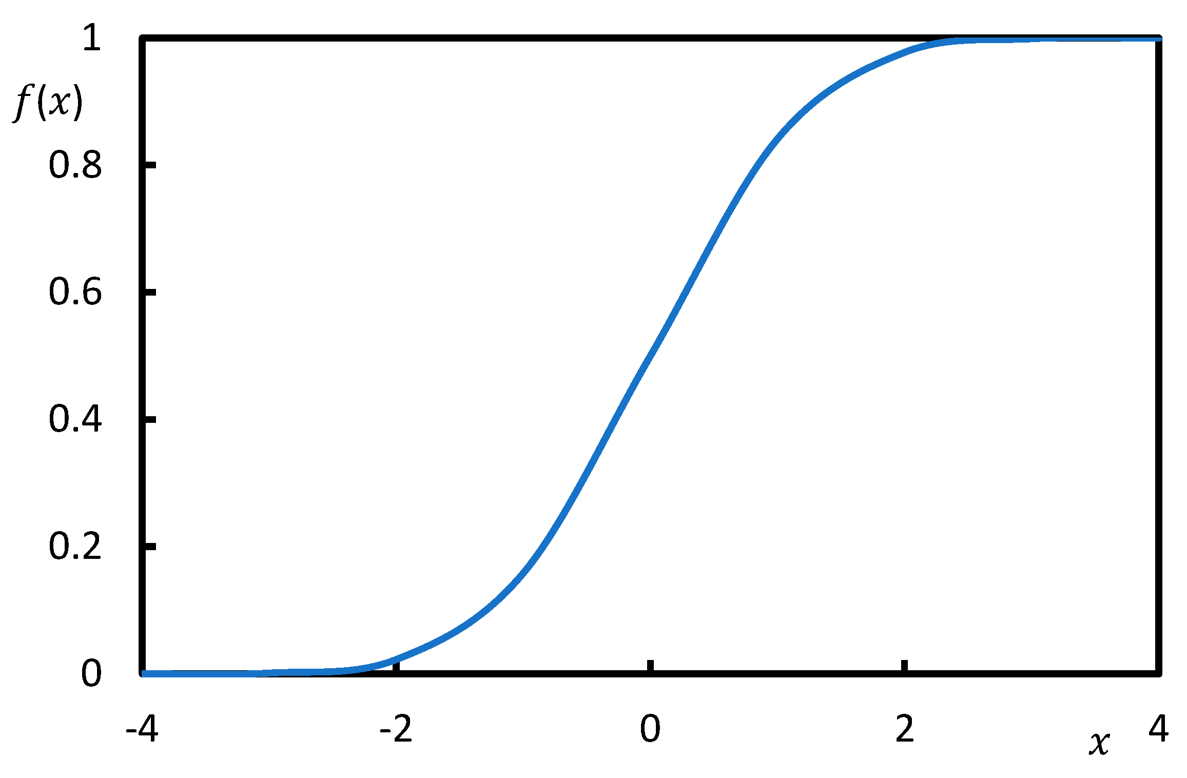
The distribution function of this variable, called the standardized variable, is expressed by the formula

$$\Phi \left(x\right)={\displaystyle \frac{1}{\sqrt{2\pi }}}\underset{-\infty }{\overset{x}{\int }}{e}^{-{\displaystyle \frac{t^2}{2}}}dt$$

(12)

Figure 6 shows the distribution function of the normal distribution $N\left(\mathrm{0,1}\right)$.

One of the most important properties of the normal distribution is that under certain assumptions, the distribution of the sum of a large number of random variables is approximately normal. This is the so-called central limit theorem, considered to be the most important theorem in mathematical statistics. It was proven in the 1920s by J.W. Lindeberg and P. Levy. It is concerned with the convergence of the sum of independent random variables with the same distributions (the distribution does not have to be known) to the normal distribution.

The proposed set of functions was selected based on previous timing studies conducted under the conditions of a given longwall face; a probability density function describing the execution times on a section of 1 m was adopted for further calculations, which proved that the selected functions described the mining process issues well. However, it is not a closed set and can be supplemented with other functions. A slightly broader concept, the concept of distribution, was used in the description of the function. If the probability density function or the distribution function is known, one can speak of knowing the distribution.

3. Results

This section presents a step-by-step methodology for reducing the stochastic model for coal output using the convolution of probability density functions.

The definition of the convolution of probability density functions is as follows [22]:

Definition 1.

If  $X$ is an independent random variable with a distribution $f_x\left(x\right)$ , and $Y$ is an independent random variable with a distribution $f_y\left(y\right)$ , then the random variable $U$   is their sum, that is,

$$U=X+y$$

(13)

has a probability distribution

$$f\left(u\right)=\underset{-\infty }{\overset{\infty }{\int }}{f}_y\left(y\right)f_x\left(u-y\right)dy$$

(14)

The integral on the right-hand side of the formula is called the convolution integral. We can therefore say that the density of the sum of independent random variables is the convolution of the density of the summed random variables, which can also be written as

$$f_{x+y}=f_x⨂f_y$$

(15)

The formula can be generalized to the case of summing any finite number of continuous random variables $W_1$, $W_2,\dots ,W_n$ obtaining

$$f_{W_1+W_2+\dots +W_n}=f_{W_1}⨂f_{W_2}⨂\dots {⨂f}_{W_n}$$

(16)

The following section presents a simple example of a stochastic model described using continuous random variables, which can be analyzed, for example, through stochastic simulation, or the model can be simplified using the properties of the convolution of probability density functions.

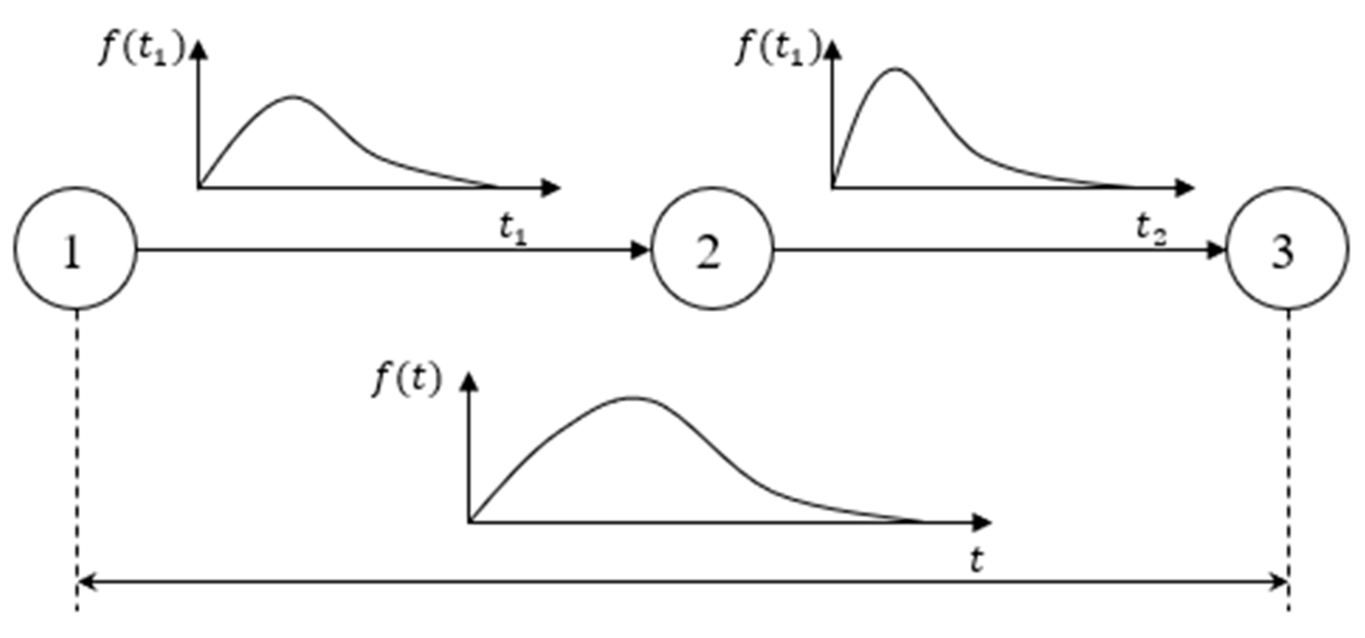
Figure 7 shows an example fragment of a stochastic model, in which the random variables describing it are continuous.

The model presents two serially performed operations, e.g., technological ones. The first operation is performed between the points marked with numbers 1 and 2, with the second occurring between 2 and 3. Each of these operations is characterized by a random variable, marked as $T_1$ and $T_2$. Their probability density functions have the symbols $f\left(t_1\right)$ and $f\left(t_2\right)$, respectively.

Let us assume that the variables T1 and T2 characterize the time of execution of serially implemented technological operations (for some reasons, this time may therefore change).

The characteristic $f\left(t\right)$ of the random variable $T$ is sought, where

$$T=T_1+T_2$$

(17)

The variable $T$ is—in this case—the total time of the execution of a fragment of the process, e.g., production, in which two technological operations are carried out in series between points 1 and 3.

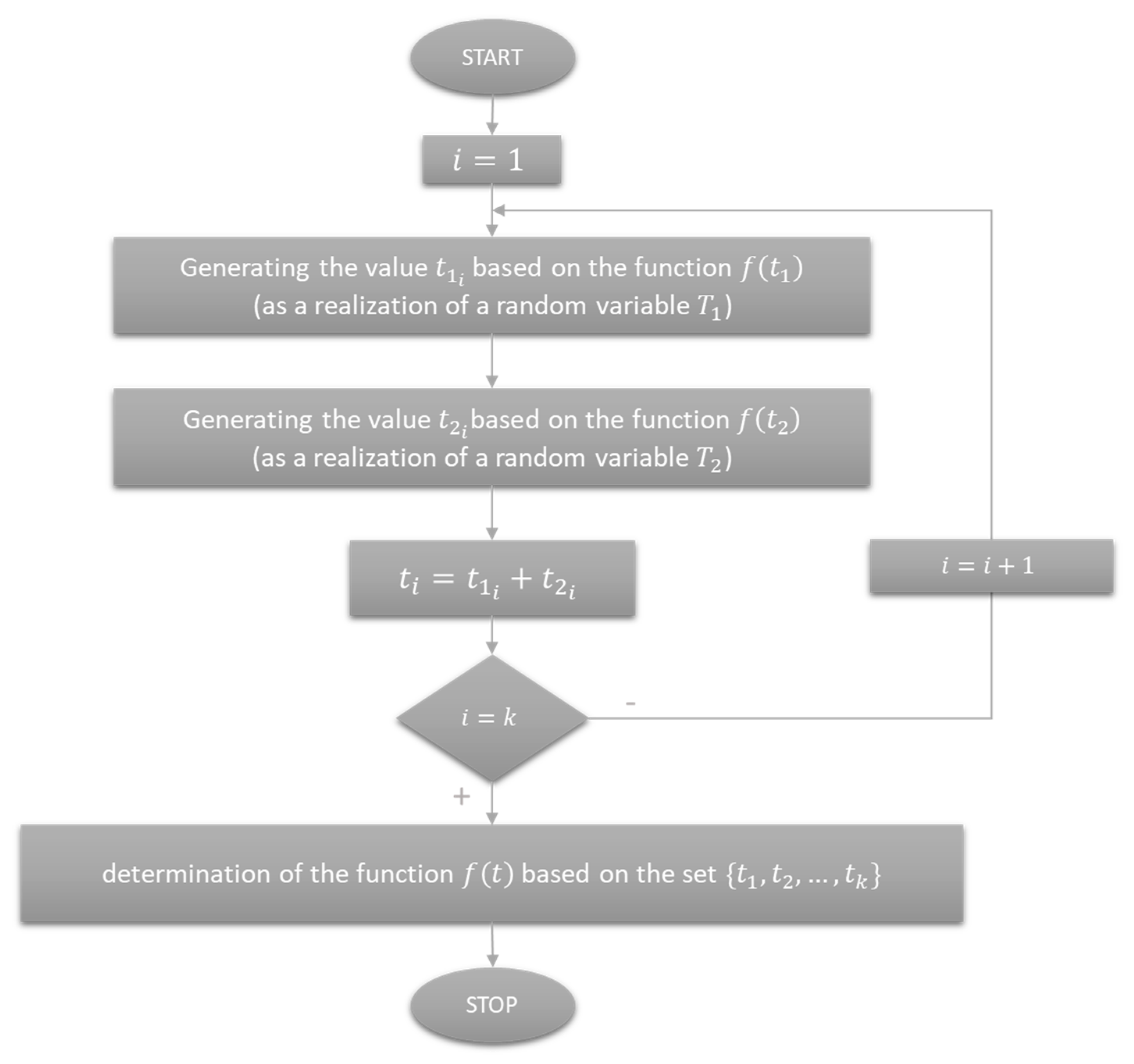
A sample algorithm for obtaining the characteristic $f\left(t\right)$ of the random variable T by means of stochastic simulation is presented in Figure 8.

A fragment of the process model presented in Figure 7 can be reduced without the need to use the stochastic simulation algorithm described in Figure 8.

The following part presents cases of model reduction using the properties of convolutions of specific types of continuous distributions (the examples concern the chi-square, gamma, and normal distributions).

The rules for selecting “$k$” were determined in accordance with the principles of statistics. A detailed description is provided in [22].

3.1. Convolution of the Chi-Square Distributions

If ${\chi }_1^2, {\chi }_2^2,\dots , {\chi }_r^2$ are independent random variables with a chi-square distribution with the parameter $n_i$ (the number of degrees of freedom) each, then the random variable ${\chi }_1^2+ {\chi }_2^2+\cdots + {\chi }_r^2$ also has a chi-square distribution with the number of degrees of freedom $n=\sum _{i=1}^r{k}_i$.

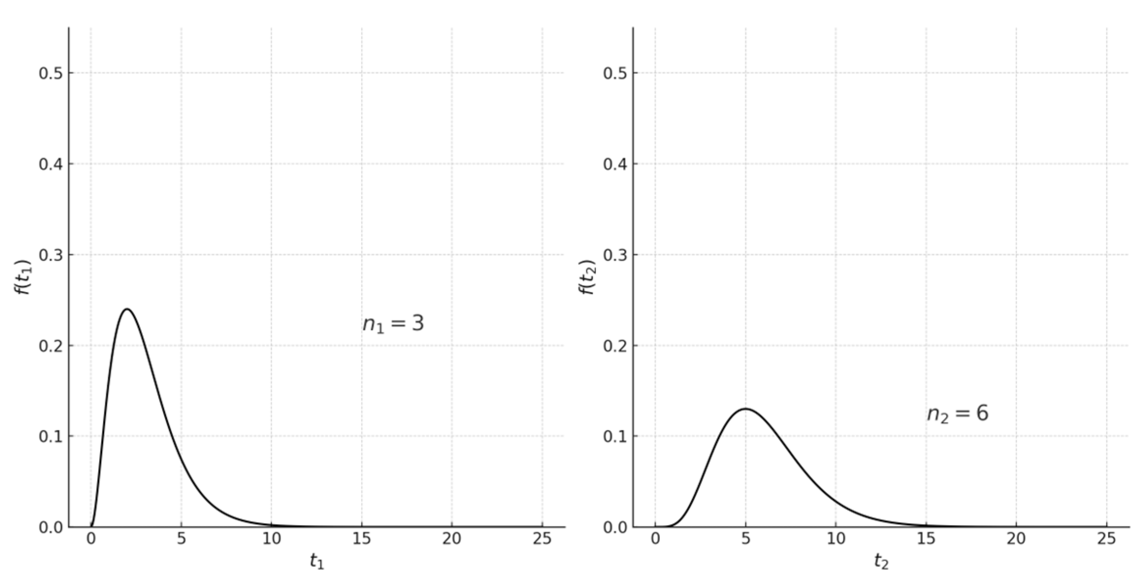
Figure 9 shows the chi-square distributions of variables $T1$ and $T2$, while Figure 10 shows the form of the function $f\left(t\right)$ variable $T=T_1+T_2$ (convolution of these distributions), which is also a chi-square distribution.

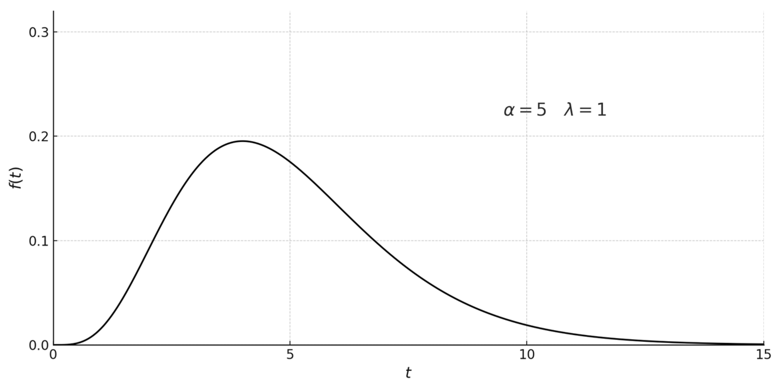
3.2. Convolution of Gamma Distributions

If $X_1, X_2, \dots , X_r$ are independent random variables with a gamma distribution with the parameters ${\alpha }_1,\lambda ; {\alpha }_2,\lambda ;\dots ; {\alpha }_r,\lambda$, then the random variable $X_1+ X_2+ \dots + X_r$ also has a gamma distribution with the parameters ${\alpha }_1+{\alpha }_2+\cdots +{\alpha }_r,\lambda$.

Figure 11 shows the gamma distributions of variables $T1$ and $T2$, while Figure 12 shows the form of the function $f\left(t\right)$ variable $T=T_1+T_2$ (convolution of these distributions), which is also a gamma distribution.

3.3. Convolution of Normal Distributions

If $X_1, X_2, \dots , X_r$ are independent random variables with a normal distribution with the parameters ${\mu }_1;{\delta }_1; {\mu }_2,{\delta }_2;\dots ; {\mu }_r,{\delta }_r$, then the random variable $X_1+ X_2+ \dots + X_r$ also has a normal distribution with the parameters $\mu ={\mu }_1+{\mu }_2+\cdots +{\mu }_r$, $\delta =\sqrt{{\delta }_1^2+{\delta }_2^2+\dots +{\delta }_r^2}$.

Figure 13 shows the normal distributions of variables $T1$ and $T2$, while Figure 14 shows the form of the function $f\left(t\right)$ variable $T=T_1+T_2$ (convolution of these distributions), which is also a normal distribution.

4. Discussion

Based on the research presented in Section 2 and Section 3, calculations were made which the authors present in this section.

We present the possibility of reducing stochastic models to create such models as an illustration of mining processes for the purpose of their further analysis in cases where the influence of geological–mining and technical–organizational conditions means that the selected process characteristics can be treated as random variables. A comprehensive description of such models and the methods for their solution are included, among others, in the works [22,23].

The example (illustrated using general formulas) is taken from [3]. The daily output is the sum of each individual shift-wise output of production on the longwall face, i.e.,

$$Q_d=\sum _{i=1}^n{Q}_{z_i}$$

(18)

where

$Q_d$—the daily output [Mg/day];

$Q_{z_i}$—the shift-wise output on the “i” shift [Mg/m];

$n$—the number of shift-wise outputs during the day [m/day].

According to the adopted assumptions, under certain conditions, the shift-wise output is treated as a random variable. The probability density of the sum of random variables is therefore the density of the marginal distribution of the variable $Q_d$, which is a convolution of the random variable functions $Q_{z_i}$, i.e.,

$$f_{q_d}=f_{q_{z_1}}⨂f_{q_{z_2}}⨂\dots ⨂f_{q_{z_n}}$$

(19)

where

$f_{q_d}$—the function of the marginal distribution density of the random variable $Q_d$ (daily output);

$f_{q_{z_1}}$—the function of the probability density of the random variable $Q_{z_1}$ (the shift-wise output on the first shift);

$f_{q_{z_2}}$—the function of the probability density of the random variable $Q_{z_2}$ (the shift-wise output on the second shift);

$f_{q_{z_n}}$—the function of the probability density of the random variable $Q_{z_n}$ (the shift-wise output on the shift “$n$”).

According to the definition of the convolution of the probability density functions and taking into account the independence of the random variables $Q_{z_1}, Q_{z_2}, \dots , Q_{z_n}$, the general formula is obtained:

$$f_{q_d}\left(q_d\right)=\underset{-\infty }{\overset{\infty }{\int }}\dots \underset{-\infty }{\overset{\infty }{\int }}{f}_{q_{z_1}}\left(q_{z_1}\right)f_{q_{z_2}}\left(q_d-q_{z_1}\right)\dots f_{q_{z_n}}\left(q_d-q_{z_1}-\cdots -q_{z_{n-1}}\right) d{q}_{z_1}d{q}_{z_1}\dots d{q}_{z_{n-1}}$$

(20)

For example, for $n=2$ (two shift-wise outputs from the longwall face from one day), the boundary function takes the form

$$f_{q_d}\left(q_d\right)=\underset{-\infty }{\overset{\infty }{\int }}\dots \underset{-\infty }{\overset{\infty }{\int }}{f}_{q_{z_1}}\left(q_{z_1}\right)f_{q_{z_2}}\left(q_d-q_{z_1}\right)d{q}_{z_1}$$

(21)

the designations were adopted as shown in Formula (6).

It can be seen that Formula (9) is identical to the formula marked as 2; hence, the stochastic model reduction described in this paper using the convolution of probability density function properties can be used to obtain the functional characteristics of the daily output from the longwall face.

The conducted study confirms the effectiveness of using the convolution properties of probability density functions to reduce stochastic models in the context of mining production processes. The traditional stochastic simulations—although accurate—are often time-consuming and computationally intensive and may require extensive input data and calibration. The reduction method presented in this paper offers a promising alternative that retains mathematical rigor while significantly simplifying the analytical procedures.

The model used in this research reflects a typical production scenario on a longwall face, where process segments—such as cutting, loading, and transport—are performed in sequential order. Each segment can be represented using a random variable, whose variability stems from geological or operational uncertainty. The convolution of these variables allows us to obtain the probability distribution of the total process duration or production volume, eliminating the need for full-scale simulation.

This approach is especially relevant in the context of modern mining challenges, where deeper deposits, harder rock conditions, and increased technical complexity contribute to greater process uncertainty. The possibility of analytically modeling the aggregated variability (e.g., the daily or shift-wise output) allows mine-planners and decision-makers to more accurately forecast the production behavior and respond more effectively to deviations.

Furthermore, the reduction technique enables clearer communication of the model’s assumptions and outputs. While stochastic simulations can sometimes function as a “black box”, analytical solutions based on known distributions (e.g., gamma, normal, chi-square) enhance the transparency and replicability. This makes the approach more accessible not only to researchers but also to practitioners without extensive statistical backgrounds.

Importantly, the reduction does not imply the loss of modeling fidelity. As shown in the examples with specific distributions, the convolution produces exact output distributions under defined assumptions (the independence, continuity, and known form of the distributions). These conditions are often met in mining applications, especially when time-based observations are used to parameterize the model.

Finally, this method has potential applications beyond coal mining. Similar techniques may be applied in other domains characterized by sequential stochastic processes, such as logistics, maintenance planning, and production in batch systems. Future work may involve the integration of this approach into decision-support systems or its combination with machine learning for hybrid modeling architectures.

5. Conclusions

These studies could be performed because the production process carried out on the longwall faces of hard coal mines takes place underground, in specific mining–geological and technical–organizational conditions that determine its specificity. Hence, an analysis of this process in order to determine the shift-wise output can be carried out using determinate or stochastic models.

The analysis of the literature conducted showed that the beginnings of creating deterministic models date back to the 1960s and that these models were developed over the following decades. The disadvantage of these models is their determinism, i.e., obtaining the desired characteristic, e.g., extraction in point form. However, practice shows that the extraction obtained is not always constant—it is subject to fluctuations. The treatment of the production process carried out on the longwall face as stochastic results from including random variables in the model.

In this paper, attention was paid to the possibilities of reducing the stochastic model based on the use of the properties of the convolution of probability density functions. Reduction carried out in this way eliminates the need to analyze these parts of the model using the stochastic simulation method. This reduction is based on the possibilities offered by the properties of the probability density function. The procedure presented in the Results section facilitates both the analysis of the model and calculations that lead to clear results.