Analytical Inertia Identification of Doubly Fed Wind Farm with Limited Control Information Based on Symbolic Regression

Abstract

The integration of large-scale wind power clusters significantly reduces the inertia level of the power system, increasing the risk of frequency instability. Accurately assessing the equivalent virtual inertia of wind farms is critical for grid stability. Addressing the dual bottlenecks in existing inertia assessment methods, where physics-based modeling requires full control transparency and data-driven approaches lack interpretability for inertia response analysis, thus failing to reconcile commercial confidentiality constraints with analytical needs, this paper proposes a symbolic regression framework for inertia evaluation in doubly fed wind farms with limited control information constraints. First, a dynamic model for the inertia response of DFIG wind farms is established, and a mathematical expression for the equivalent virtual inertia time constant under different control strategies is derived. Based on this, a nonlinear function library reflecting frequency-active power dynamic is constructed, and a symbolic regression model representing the system’s inertia response characteristics is established by correlating operational data. Then, sparse relaxation optimization is applied to identify unknown parameters, allowing for the quantification of the wind farm’s equivalent virtual inertia. Finally, the effectiveness of the proposed method is validated in an IEEE three-machine nine-bus system containing a doubly fed wind power cluster. Case studies show that the proposed method can fully utilize prior model knowledge and operational data to accurately assess the system’s inertia level with low computational complexity.

1. Introduction

The rapid integration of renewable energy sources such as wind and solar power is progressively replacing traditional thermal generation, significantly depleting power system inertia [1,2,3]. The “near-zero inertia” characteristics of grid-connected wind turbines critically undermine frequency stability during contingencies [4,5,6,7], as evidenced by major blackouts in South Australia (2016) [8,9] and the UK (2019) [10]. In response to this challenge, both manufacturers of wind turbines and operators of electrical grids have prioritized the development of inertia control technologies [11,12,13,14,15,16,17,18,19], particularly through virtual inertia control and integrated inertia control. Therefore, the accurate quantification of wind farms’ equivalent virtual inertia under diverse control strategies [20,21] has emerged as a pivotal enabler for deploying effective frequency stability countermeasures in low-inertia systems [22,23].

A considerable number of researchers have investigated the inertia characteristics of wind farms, grounded in physical principles and data-driven methodologies. Ref. [24] formulated the voltage phase angle motion equation for DFIGs, thereby providing a representation of the equivalent virtual inertia of the wind farms. It has been noted that the equivalent virtual inertia of a wind farm is a variable quantity that changes over time, and its magnitude is associated with the control parameters employed; Ref. [25] represented the equivalent inertia time constant of a wind turbine as a function of the wind rotor inertia, the initial operating point of the turbine, and rotor speed variations, while the equivalent virtual inertia time constant is expressed as a piecewise linear function of wind speed. It also emphasizes that the wind farm inertia response is closely tied to the turbine’s operating conditions. These studies derived the equivalent virtual inertia of wind farms from a physical mechanism perspective and further deepened our understanding of wind farm equivalent virtual inertia. Nevertheless, these methods require precise knowledge of each wind turbine’s control parameters and structure, making them challenging to apply when the information is unavailable.

Recent advancements in wide-area measurement technologies and artificial intelligence algorithms have facilitated the widespread adoption of data-driven methodologies for assessing wind farm inertia [26,27,28]. In the process of selecting an identification model, the detailed ontology-based modeling approach based on physical mechanisms establishes explicit mathematical relationships between inertial response characteristics and control parameters through the integration of prior knowledge, providing a theoretical foundation for quantifying equivalent virtual inertia characteristics in wind farms. Studies such as ref. [29] utilized the Kalman filter to identify the control parameters within wind turbine structures, integrating this with inertia calculations to evaluate the inertia of the wind farm. Ref. [30] derived the active power-frequency transfer function of wind power based on the physical connections of various control modules within the wind farm. Using measured active power–frequency curves, the parameters of the transfer function are identified through the least squares method, thereby obtaining the equivalent inertia coefficient.

Due to commercial confidentiality, manufacturers of renewable energy equipment typically provide only black-box models, which delineate input–output characteristics. The internal control structure is generally considered proprietary and is not readily accessible. Consequently, the development of a polynomial model to delineate the input–output relationship is a widely adopted methodology for addressing this concern. Ref. [31] established a polynomial model based on measured active power–frequency disturbance data and, combined with the swing equation principle, derived the equivalent virtual inertia of the wind farm. Ref. [32] developed a controlled autoregressive model, employing recursive least squares to estimate the time-varying inertia of DFIGs. However, both methods generally necessitate the presence of external disturbance signals and are unable to leverage steady-state operational measurement data for estimation. In response to this, ref. [33] proposes a novel data-driven method using ambient measurements, which seems to be a method that can estimate the virtual inertia constants of CIGs simultaneously without disturbing the system’s normal operating condition. Refs. [34,35] applied a multi-input multi-output autoregressive moving average model to determine the system inertia co-efficient in the presence of small-signal disturbances in the environment. Nevertheless, the assessment and analysis of the equivalent virtual inertia of the wind farm are not encompassed within this study. Meanwhile, the above methods share a common limitation in that the evaluation accuracy depends significantly on the selection of the model order and the identified models lack explicit analytical expressions, thereby restricting their applicability in detailed inertia response analysis.

In conclusion, contemporary methodologies for assessing wind farm inertia encounter several obstacles, including restricted access to control structures and parameters due to commercial confidentiality (the control information of wind turbines is limited), as well as limited applicability to inertia response analysis. To address these issues, this paper introduces a symbolic regression approach for inertia assessment. Initially, modules pertinent to inertia response are classified and associated with extensive operational data, employing sparse dynamic modeling to develop a nonlinear feature library that captures frequency-active power variations. Following this, a sparse relaxation optimization algorithm is utilized to regress the control parameters, enabling the calculation of the wind farm’s inertia through the equivalent virtual inertia expression applicable to doubly fed wind farms. The efficacy of this method is subsequently validated through simulations conducted on the IEEE three-machine nine-bus system.

The organization of this paper is delineated as follows: Section 2 introduces the mathematical framework governing DFIG, alongside two prevalent inertia control methodologies, and the limited control information of wind turbines is defined; it subsequently formulates the analytical expression for the equivalent virtual inertia of DFIG, considering various control strategies. Section 3 constructs an inertia response model of DFIG with limited control information utilizing sparse dynamic modeling. Section 4 employs the sparse relaxed regularization (SR3) algorithm for the identification of model parameters, which are subsequently utilized to evaluate the inertia of the wind farm. Section 5 presents a comparative analysis of the identified equivalent virtual inertia against simulation outcomes across diverse conditions. Finally, Section 6 encapsulates the benefits of the pro-posed methodology and delineates prospective avenues for future research.

2. Modeling and Analytical Benchmarking of Equivalent Virtual Inertia for DFIGs

2.1. Dynamic Model of DFIG with Inertia Control Methods

In the synchronous reference frame, the DFIG model with stator flux orientation is represented by a simplified fifth-order mathematical model, including flux, electromagnetic torque, and rotor motion equations.

$$\left\{\begin{array}{l}{\psi }_{d,s}=L_s{i}_{d,s}+L_m{i}_{d,r}={\psi }_s\\ {\psi }_{q,s}=L_s{i}_{q,s}+L_m{i}_{q,r}=0\end{array}\right.$$

(1)

$$P_e={\displaystyle \frac{3p{L}_m}{4{\omega }_s{L}_s}}{\psi }_{d,s}{i}_{q,r}$$

(2)

$$2H_{wind}{\displaystyle \frac{d{\omega }_r}{dt}}=P_m-P_e$$

(3)

where ${\psi }_s$ is the stator flux linkage; ${\psi }_{d,s}$ is the d-axis component of ${\psi }_s$; ${\psi }_{q,s}$ is the q-axis component of ${\psi }_s$; $i_{d,s}$, $i_{d,r}$, $i_{q,s}$ and $i_{q,r}$ are the d-axis and q-axis components of the currents in the stator and rotor windings, respectively; $L_m$ is the mutual inductance between the stator and rotor; $L_s$ is the stator self-inductance; $p$ is the number of pole pairs of the wind turbine; ${\omega }_s$ is the grid angular frequency; ${\omega }_r$ is the rotor speed; $H_{wind}$ is the inherent inertia time constant of the WT; $P_m$ is the mechanical power of the WT; and $P_e$ is the electromagnetic power of the WT.

To enhance the frequency stability of power systems, DFIGs are often equipped with supplementary inertia control strategies. Among them, virtual inertia control [36,37] and integrated inertia control [38] are widely implemented in practical wind power applications. Consequently, they are selected in this work as representative cases to evaluate the effectiveness and applicability of the proposed identification methodology under limited model transparency.

The virtual inertia control involves the incorporation of a frequency differential signal into the RSC, which facilitates dynamic adjustments to the rotor speed and active power output, thereby emulating the inertia response characteristic of synchronous machines; this can be expressed as follows:

$$\mathsf{\Delta }{P}_1^{\ast }=-k_{d_1}\left({\displaystyle \frac{\mathsf{\Delta }{\omega }_s\cdot s}{1+T_f\cdot s}}\right)$$

(4)

where $\mathsf{\Delta }{\omega }_s$ is the change in angular frequency; $k_{d1}$ is the virtual inertia control gain; and $T_f$ is the time constant of the low-pass filter.

The integrated inertia control combines virtual inertia control and droop control. It adjusts the WT power output based on frequency deviation and the rate of change. When the grid frequency exceeds nominal, the power command becomes negative, reducing output and accelerating the rotor. During a frequency drop, the rotor slows, converting kinetic energy into active power for short-term grid support; this can be derived as follows:

$$\mathsf{\Delta }{P}_2^{\ast }=-k_p\mathsf{\Delta }{\omega }_s-k_{d2}\left({\displaystyle \frac{\mathsf{\Delta }{\omega }_s\cdot s}{1+T_f\cdot s}}\right)$$

(5)

where $k_p$ and $k_{d2}$ represent the proportional and derivative coefficients of the combined inertia control, respectively.

Meanwhile, the transfer function expressions for the reference electromagnetic power under MPPT module are given as follows [39]:

$$\mathsf{\Delta }{P}_3^{\ast }=\mathsf{\Delta }{\omega }_r\left(k_{p1}+{\displaystyle \frac{k_{i1}}{s}}\right)$$

(6)

where $\mathsf{\Delta }{P}_3^{\ast }$ is the reference electromagnetic power under the MPPT module; $\mathsf{\Delta }{\omega }_r$ is the change in the wind turbine rotor speed; $k_{i1}$ and $k_{p1}$ are the integral and proportional gains of the speed controller, respectively.

Figure 1 shows the simplified DFIG model under different inertia control strategies. Considering that the current inner loop responds much faster than the electromechanical transient process of the generator, the converter’s inner loop is simplified as a first-order inertia element in this study: $G_s(s)=1/\left(\tau s+1\right)$, $\tau$ is the converter time constant.

2.2. Analytical Derivation of Equivalent Inertia Time Constant

The virtual inertia time constant of a wind turbine is defined by the ratio of kinetic energy stored at the rated rotor speed to the generator’s rated capacity and can be formulated as follows [32,40]:

$$H\hspace{1em}={\displaystyle \frac{E_k}{S_N}}={\displaystyle \frac{1}{2}}{\displaystyle \frac{{\omega }_{s0}^2{J}_{eq}}{S_N}}={\displaystyle \frac{{\omega }_{s0}{\omega }_{r0}}{{\omega }_N^2}}{\displaystyle \frac{\mathsf{\Delta }{\omega }_r}{\mathsf{\Delta }{\omega }_s}}{H}_{wind}$$

(7)

where $E_k$ represents the kinetic energy stored in the generator rotor at the rated speed of a single wind turbine; $S_N$ is the rated capacity of the wind turbine; ${\omega }_N$ is the rated angular frequency of the wind turbine; ${\omega }_{s0}$ and ${\omega }_{r0}$ are the initial grid angular frequency and initial generator speed, respectively; and $J_{eq}$ is the virtual equivalent moment of inertia of the wind turbine.

Subsequently, the equivalent virtual inertia time constants corresponding to the two control strategies can be derived individually [41].

$$H_1\left(s\right)={\displaystyle \frac{H_{wind}{\omega }_{s0}{\omega }_{r0}{k}_{d1}{s}^2}{{\omega }_N^2\left(1+T_f\cdot s\right)\left(2H_{wind}{s}^2+k_{p1}s+k_{i1}\right)}}$$

(8)

$$H_2\left(s\right)={\displaystyle \frac{H_{wind}{\omega }_{s0}{\omega }_{r0}\left(k_{d2}s+k_p\right)s}{{\omega }_N^2\left(1+T_f\cdot s\right)\left(2H_{wind}{s}^2+k_{p1}s+k_{i1}\right)}}$$

(9)

where $H_1$ denotes the equivalent virtual inertia time constant under virtual inertia control, and $H_2$ represents the equivalent virtual inertia time constant under integrated inertia control.

The above equation is the method for calculating the inertia time constant of a single wind turbine. For a wind farm consisting of n DFIG units, the wind farm can be equivalently represented as a single aggregated unit, with the equivalent virtual inertia given as follows [32]:

$$\begin{array}{l}{H}_{eq}={\displaystyle \frac{{\displaystyle \sum _{j=1}^n{E}_{kj}}}{{\displaystyle \sum _{j=1}^n{S}_{Nj}}}}={\displaystyle \frac{\frac{J_{equ1}{\omega }_{s0}^2}{2}+\frac{J_{equ2}{\omega }_{s0}^2}{2}+\dots +\frac{J_{equn}{\omega }_{s0}^2}{2}}{S_{N1}+S_{N2}+\dots +S_{N\mathrm{n}}}}=\\ {\displaystyle \frac{H_{equ1}{S}_{N1}+H_{equ2}{S}_{N2}+\dots +H_{equ\mathrm{n}}{S}_{Nn}}{S_{N1}+S_{N2}+\dots +S_{Nn}}}=\\ {\displaystyle \frac{{\displaystyle \sum _{j=1}^n{H}_{equj}}{S}_{Nj}}{{\displaystyle \sum _{j=1}^n{S}_{Nj}}}}={\displaystyle \frac{{\displaystyle \sum _{j=1}^n{H}_{equj}}}{n}}\end{array}$$

(10)

where $H_{eq}$ is the equivalent virtual inertia of the wind farm; $H_{equj}$ is the virtual inertia of a single WT.

By substituting Equation (10) into Equation (9), the frequency expression for the equivalent virtual inertia of the wind farm with integrated inertia control can be derived as follows:

$$H_{eq}\left(s\right)={\displaystyle \frac{H_{wind}{\omega }_{s0}{\omega }_{r0}\left(k_{d2}s+k_p\right)s}{{\omega }_N^2\left(1+T_f\cdot s\right)\left(2H_{wind}{s}^2+k_{p1}s+k_{i1}\right)}}\cdot {\displaystyle \frac{{\displaystyle \sum _{j=1}^n{\omega }_{r0j}}}{n}}$$

(11)

where ${\omega }_{r0j}$ is the initial angular velocity of the jth WT.

Based on Equation (11), the equivalent virtual inertia of wind farms is time-varying, depending on the control parameters, inherent inertia time constant, and operational conditions. Typically, ${\omega }_N$ can be obtained from the generator’s technical manual; ${\omega }_{s0}$ can be measured in real-time. Meanwhile, ${\omega }_{r0}$ equals the reference rotor speed ${\omega }_{ref}$ under steady-state conditions, which is derived from the power–speed curve. However, due to commercial confidentiality, in practice, the relevant inertia controller structure and parameters of some wind turbines are usually unknown. Therefore, the accurate evaluation of the DFIG wind farm’s equivalent virtual inertia requires the inertia control structure and parameters of the WT to be identified.

2.3. The Model Overview of DFIG with Limited Control Information

To solve the above problems, this paper proposes the “limited control information” framework, which categorizes wind turbine control knowledge through a hierarchical dual-layer structure in Figure 1, explicitly distinguishing between parametric identifiability (Gray Frame) and structural identifiability (Colored Frame). In this framework, a “module” refers to a functionally independent subsystem within the wind energy conversion system, each characterized by different levels of structural transparency and parameter accessibility. The system is decomposed into the following modules:

(1)

Known Structural Layer: including modules whose functional structures are known from theory but whose parameters must be identified from data. This layer comprises the induction machine, rotor dynamics, and maximum power point tracking (MPPT) modules. These components exhibit a high degree of consistency with standard DFIG models and can be modeled using established physical equations with unknown coefficients.

(2)

Unknown Structural Layer: including the inertia control module, whose internal structure and control logic are not disclosed due to manufacturer confidentiality. As such, this module is treated as a black box, requiring both structural and parametric identification through input–output data.

3. Sparse Dynamic Modeling and Convex Regression for Inertia Response

3.1. Fundamentals of Sparse Dynamic Modeling

Generally, the operational data for each module is dictated by its mathematical formulation, which can be represented as $\dot{\mathit{x}}={\mathit{f}}_i\left(\mathit{x},\dot{\mathit{x}},\mathit{u},\mathit{p}\right)$, where the right-hand side includes inputs $\mathit{u}$, parameters $\mathit{p}$, and state variables $\mathit{x}$, along with their rates of change $\dot{\mathit{x}}$.

The operational data for each module is gathered and depicted as a sequence in the time domain:

$$X={\left\{\mathit{x}\left(1\right),\mathit{x}\left(2\right),\mathit{x}\left(3\right)\dots \mathit{x}\left(n\right)\right\}}^T$$

(12)

where $X$ is an $n\times m$ data matrix, $m$ is the number of state variables and $n$ is the number of data points collected. The rate of change of the operating variables at $i=t$ is further calculated using numerical methods, denoted as ${\dot{X}}_i$.

After obtaining the operating data and based on the dynamic equations of each module, a linear/nonlinear function library $\Theta$ is constructed to reflect ${\mathit{f}}_i$ the dynamic characteristics, such that:

$$\dot{\mathit{x}}={\mathit{f}}_i\left(\mathit{x},\dot{\mathit{x}},\mathit{u},\mathit{p}\right)={\Theta }_i\left({\mathit{x}}^T,{\dot{\mathit{x}}}^T,{\mathit{u}}^T\right)\mathit{\xi }$$

(13)

where $\mathit{x}$, $\dot{\mathit{x}}$ and $\mathit{u}$ are symbolic variables, and $\mathit{\xi }$ is the coefficient of the corresponding term in the function library, which corresponds to the original equation parameters. This can be further transformed into matrix form as follows:

$$\dot{\mathit{x}}={\mathit{f}}_i\left(\mathit{x},\dot{\mathit{x}},\mathit{u},\mathit{p}\right)={\Xi }^T{\left({\Theta }_i\left({\mathit{x}}^T,{\dot{\mathit{x}}}^T,{\mathit{u}}^T\right)\right)}^T$$

(14)

where $\Xi =\left[{\mathit{\xi }}_1,{\mathit{\xi }}_2,\dots {\mathit{\xi }}_n\right]$ and ${\Theta }_i\left({\mathit{x}}^T,{\dot{\mathit{x}}}^T,{\mathit{u}}^T\right)$ are composed of combinations of $\mathit{x}$, $\dot{\mathit{x}}$, $\mathit{u}$. The combinations can take the form of first- or higher-order polynomials, trigonometric functions, or other types of nonlinear function representations.

3.2. The Methodology of Sparse Dynamic Modeling for DFIGs with Limited Control Information

3.2.1. Model-Prior-Integrated Sparse Dynamic Modeling with Matrix Constraints

For example, the rotor motion equation in a doubly fed wind turbine can be expressed as a linear equation, as follows:

$$2H_{wind}{\displaystyle \frac{d{\omega }_r}{dt}}=T_m-T_e$$

(15)

Equation (15) can be reformulated into the standard form of Equation (13): the state variable ${\omega }_r$ is replaced with $x_1$, and the input variables $T_e$ and $T_m$ are replaced with $u_1$, $u_2$ respectively. At this point, the equation can be re-formulated as follows:

$$\dot{\mathit{x}}={\displaystyle \frac{u_2}{2H_{wind}}}-{\displaystyle \frac{u_1}{2H_{wind}}}$$

(16)

In Equation (16), the terms on the right-hand side that depend on the state variables $x$ and the module inputs $u$ are assumed to follow prescribed functional forms. These terms are regarded as a unified entity for the purpose of constructing a linear candidate function library:

$$\dot{\mathit{x}}={\Xi }^T\Theta {\left(u_1,u_2\right)}^T$$

(17)

Given the known model structure, the coefficients associated with the nonlinear terms on the right-hand side can be predetermined and represented in matrix form:

$$\Xi \left(u_1,{\dot{x}}_1\right)+\Xi \left(u_2,{\dot{x}}_1\right)=0$$

(18)

Similarly, based on the nonlinear dynamic’s equations of the DFIG, $x={\left[x_1 x_2 x_3 x_4\right]}^T={\left[i_{dr} i_{qr} i_{ds} i_{qs}\right]}^T$; $u={\left[u_1 u_2 u_3 u_4 u_5\right]}^T={\left[u_{dr} u_{qr} u_{ds} u_{qs} {\omega }_r\right]}^T$. This results in the construction of the (non)linear feature library as follows:

$$\dot{\mathit{x}}={\Xi }^T\Theta {\left(\mathit{x},\mathit{u},\mathit{x}\otimes u_5\right)}^T$$

(19)

where $\mathit{u}$ is the input vector, and $\otimes$ denotes the vector combination of the elements on both sides of the operator.

Since the DFIG’s induction motor in the black-box model closely matches the theoretical structure, it is treated as known. Accordingly, the parameters in the nonlinear function library are fixed using matrix constraints, as shown:

$$\begin{array}{l} \Xi \left(x_2,{\dot{x}}_3\right)+\Xi \left(x_1,{\dot{x}}_4\right)=0\\ \Xi \left(x_4,{\dot{x}}_3\right)+\Xi \left(x_3,{\dot{x}}_4\right)=0\\ \Xi \left(u_5\otimes x_2,{\dot{x}}_1\right)+\Xi \left(u_5\otimes x_1,{\dot{x}}_2\right)=0\\ \Xi \left(u_5\otimes x_4,{\dot{x}}_1\right)+\Xi \left(u_5\otimes x_3,{\dot{x}}_2\right)=0\\ \Xi \left(x_1,{\dot{x}}_1\right)=\Xi \left(x_2,{\dot{x}}_2\right);\Xi \left(x_3,{\dot{x}}_3\right)=\Xi \left(x_4,{\dot{x}}_4\right)\\ \Xi \left(u_1,{\dot{x}}_1\right)=\Xi \left(u_2,{\dot{x}}_2\right)=\Xi \left(u_3,{\dot{x}}_3\right)=\Xi \left(u_4,{\dot{x}}_4\right)\end{array}$$

(20)

Analogously, for the maximum power tracking module, the state variable ${\omega }_r$ is replaced with $x_1$, and the input variable $\mathsf{\Delta }{P}_3^{\ast }$ is replaced with $u_1$, constructing the corresponding function library as follows:

$$\dot{\mathit{x}}={\Xi }^T\Theta {\left(u_1,x_1\right)}^T$$

(21)

For convenience of analysis, the model constraints are unified into a matrix equation as follows: $C\mathit{\xi }=d$.The equation constraint correspondence is shown in Figure 2.

3.2.2. Sparse Dynamic Modeling of Unknown Inertia Control Structures

For the unknown inertia control structure, a sparse model is constructed to describe the relationship between the system state variables and input disturbance electromagnetic power, as follows:

$${\displaystyle \frac{d\mathsf{\Delta }f}{dt}}=\Theta (X)\Xi$$

(22)

The function library $\Theta (X)$ comprises a curated selection of fundamental functions, which results in the subsequent identification model:

$$\Theta (X)=\left[\mathsf{\Delta }f,\mathsf{\Delta }P,\mathsf{\Delta }f\cdot \mathsf{\Delta }P,{\displaystyle \int \mathsf{\Delta }fdt},\mathsf{\Delta }\dot{P}\right]$$

(23)

$$\stackrel{.}{X}=\Theta (X,U)\Xi$$

(24)

3.3. Model Parameter Regression Based on Convex Optimization

By incorporating the operational data obtained from each module into Equation (14), the coefficient matrix of the final identification model, or the resolution of the unknown parameters within the model, can be reformulated as a regression problem as follows:

$$\begin{array}{l}mi{n}_{\Xi ,W}{\displaystyle \frac{1}{2}}{‖\stackrel{.}{X}-\Theta (X)\Xi ‖}^2+\lambda R(W)\\ s.t.\hspace{1em}C\mathit{\xi }=d\hspace{1em}\mathit{\xi }=\Xi (:)\end{array}$$

(25)

where $R$ represents the sparsity regularization operator, chosen as the ${\mathcal{l}}_0$ norm to ensure the problem remains convex; $\lambda$ is the optimization hyperparameter used to control the sparsity level of the model.

4. Inertia Identification of Wind Farms Based on Analytical Optimization

4.1. Sparse Relaxed Regularization Algorithm

In the identification model described above, $\Xi =\left[{\xi }_1,{\xi }_2,\dots {\xi }_n\right]$ is the parameter matrix to be determined, which requires the selection of an appropriate identification algorithm for estimation. The most common method employed in this context is the LASSO (Least Absolute Shrinkage and Selection Operator) sparse regularization algorithm [42], which incorporates a regularization term to mitigate the risk of overfitting; however, it faces challenges in effectively selecting sparsity. Alternatively, the Sequential Thresholded Least Squares (STLS) [43] method integrates least squares with stepwise thresholding to iteratively enhance sparsity optimization. Nonetheless, this approach is associated with significant computational complexity, as it necessitates the repeated resolution of the least squares problem.

To enhance robustness and efficiency, the SR3 algorithm [44] has been employed to determine the parameters, resulting in the derivation of an analytical iterative expression. The optimization problem is restructured by the introduction of an auxiliary variable $W$, leading to the following formulation:

$$\begin{array}{l}mi{n}_{\Xi ,W}{\displaystyle \frac{1}{2}}{‖\stackrel{.}{X}-\Theta (X)\Xi ‖}^2+\lambda R(W)+{\displaystyle \frac{1}{2\nu }}{‖\Xi -W‖}^2\\ s.t.\hspace{1em}C\xi =d, \xi =\Xi (:)\end{array}$$

(26)

where ${\displaystyle \frac{1}{2\nu }}{‖\Xi -W‖}^2$ is the regularization penalty term that governs the disparity between the sparse solution $\xi$ and the relaxation variable $W$.

In addressing this regression issue, the “divide–relax” strategy decomposes the original problem into subproblems, optimizing $\xi$ and $W$ alternately. A vectorization equation is presented to reformulate the SR3 optimization as a linear system, as follows:

$$\left[\begin{array}{cc}{\Theta }_X^T\otimes {\Theta }_X+{\displaystyle \frac{1}{\nu }}I& C^T\\ C& 0\end{array}\right]\left[\begin{array}{c}\xi \\ \varphi \end{array}\right]=\left[\begin{array}{c}{\Theta }_X^T\otimes \stackrel{.}{X}+{\displaystyle \frac{1}{\nu }}{W}^{k-1}\\ d\end{array}\right]$$

(27)

where $\varphi$ is the Lagrange multiplier, ${\Theta }_X^T=I\otimes \Theta$, and $\otimes$ is tensor operators.

Employing the identity of the Kronecker product along with associated equations,

$${\left({\Theta }_X^T\otimes {\Theta }_X+{\displaystyle \frac{1}{\nu }}I\right)}^{-1}={\left(\Theta (X{)}^T\Theta (X)+{\displaystyle \frac{1}{\nu }}I\right)}^{-1}$$

(28)

Consequently, by addressing the aforementioned matrix equation,

$$\varphi ={\left(C{\left(\Theta (X{)}^T\Theta (X)+{\displaystyle \frac{1}{\nu }}I\right)}^{-1}\otimes I{C}^T\right)}^{-1}RHS$$

(29)

$$RHS=d-C{\left({\Theta }_X^T\otimes {\Theta }_X+{\displaystyle \frac{1}{\nu }}I\right)}^{-1}\left({\Theta }_X^T\otimes \stackrel{.}{X}+{\displaystyle \frac{1}{\nu }}{W}^{k-1}\right)$$

(30)

$$\xi ={\left({\Theta }_X^T\otimes {\Theta }_X+{\displaystyle \frac{1}{\nu }}I\right)}^{-1}\left({\Theta }_X^T\otimes \stackrel{.}{X}+{\displaystyle \frac{1}{\nu }}{W}^{k-1}-C^T\varphi \right)$$

(31)

The specific algorithm procedure is presented in Algorithm 1:

Algorithm 1: SR3

Input: Matrix $\Theta$$\mathrm{and} \stackrel{.}{X}$; Initial value: $W^0$, Constraint matrices: $C$, $d$, Hyperparameters $\lambda$, $\nu$, $\epsilon$ Output: The sparse matrix $\Xi$. Initialization$: k=0,err=2\epsilon$. Steps: While err > $\epsilon$ do $k\leftarrow k+1$ $H_k\leftarrow {\left({\Theta }_X^T\otimes {\Theta }_X+{\displaystyle \frac{1}{\nu }}I\right)}^{-1}$ $r_k\leftarrow d-C{H}_k\left({\Theta }_X^T\otimes \stackrel{.}{X}+{\displaystyle \frac{1}{\nu }}{W}^{k-1}\right)$ ${\varphi }_k\leftarrow {\left(C{H}_k{C}^T\right)}^{-1}{r}_k$ ${\xi }_k\leftarrow H_k\left({\Theta }_X^T\otimes \stackrel{.}{X}+{\displaystyle \frac{1}{\nu }}{W}^{k-1}-C^T{\varphi }_k\right)$ ${\Xi }_k=reshape({\xi }_k)$ $W^k=pro{x}_{\lambda /\nu }({\Xi }_k)$ $\mathrm{err}=\Vert W^k-W^{k-1}\Vert /\nu$ End

Therefore, the control parameters of each controller can be identified, leading to the derivation of the analytical expression for the inertia time constant of the wind farm.

4.2. Specific Steps for Identification Control Parameter and Structure

The steps for estimating the equivalent inertia of the wind farm are outlined as follows:

Step 1: Acquire and preprocess system disturbance time-series data to establish an optimized dataset ensuring analytical accuracy;

Step 2: By integrating the dynamic equations corresponding to each module, a suitable library of feature functions is chosen to develop the sparse identification model. Subsequently, the parameters of the model are determined utilizing the algorithm described in Step 3;

Step 3: Based on the SR3 algorithm in Section 4.1, the identification process involves splitting the optimization problem into data fitting and sparse regularization. Ridge regression is used for initial sparse matrix estimation, followed by the application of iterative thresholding to the relaxation variables, ultimately yielding the frequency domain expression for the wind farm’s inertia time constant;

Step 4: Compare the identified control parameters and structure with those set in the actual simulation to evaluate the model fitting accuracy and the reliability of the identification. The specific procedure is illustrated in Figure 3.

4.3. Analytical Inertia Identification of Wind Farms

Following the identification of the wind farm’s control structure and key parameters via the SR3 algorithm, the equivalent virtual inertia is quantitatively evaluated using the analytical expression derived in Section 2. Specifically, the identified virtual inertia parameters, low-pass filter time constant and so on are substituted into the expression to obtain the equivalent virtual inertia under the given control strategy.

This method bridges the data-driven identification results with theoretical models, ensuring both physical consistency and interpretability. It enables a straightforward and accurate evaluation of the wind farm’s inertial support capability under different control strategies.

5. Case Studies

The IEEE three-machine nine-bus system is modeled in MATLABR2018b/Simulink, as shown in Figure 4. A 90 MW wind farm, consisting of 60 DFIGs with virtual inertia control and integrated inertia control (1.5 MW each), substitutes for one of the synchronous generators [45,46,47]. Simulations are conducted using the average wind speed of the farm to validate the proposed inertia assessment method for wind farms based on symbolic regression. Detailed system parameters are provided in Appendix A. At t = 10 s, a sudden increase in the Load1 is applied to simulate frequency disturbance conditions for the wind farm. The total simulation time is set to 35 s. The entire simulation process was carried out on a personal computer with the following hardware specifications: Device name (From China Lenovo): LAPTOP-9BO9BDEO; Processor: AMD Ryzen 7 4800 H with Radeon Graphics @ 2.90 GHz; RAM: 16.0 GB (15.4 GB usable); GPU: NVIDIA GeForce GTX 1650 (4 GB).

5.1. Controller Structure and Parameter Identification

The identification methodology leverages wind farm inertia response data from frequency disturbances, where simulation datasets vary with control strategies and are integrated into an iterative optimization framework (partially shown in Figure 5). After obtaining the model data, this paper sets the hyperparameters based on the reference [44], $\lambda$ = 0.005 (sparsity regularization coefficient, promoting sparse model structures), $\nu$ = 5 (optimize hyperparameters to control the distance between auxiliary variables and the sparse matrix), $\epsilon$ = 1 × 10⁻⁴ (stopping criterion), and limit the maximum number of iterations to 2000. A nonlinear feature library was developed containing frequency deviation, its derivative, active power deviation, the power change rate and frequency–power product term, ensuring the physically consistent identification of virtual/synthetic inertia dynamics. The training accuracy and time of each module of the wind turbine at 9 m/s are shown in

Table 1. Training accuracy and time for each module.

Module	The Number of Iterations	Training Time	Training Accuracy
Swing equation	30	0.58	1.000
Induction motors	2000	3.15	0.999
Speed controller	46	1.54	1.000
Virtual inertia controller	1452	2.54	0.986
Integrated inertia controller	1654	2.78	0.964

. Key control structures and parameters are quantitatively identified in

Table 2. Feature library and selection for virtual/integrated inertia control structure identification.

Characteristic Items	Mathematical Expressions	Virtual Inertia Control	Integrated Inertia Control
Frequency Deviation	$\mathsf{\Delta }f$	×	✔
Rate of change in frequency	${\displaystyle \frac{d\mathsf{\Delta }f}{dt}}$	×	×
Power Output Deviation	$\mathsf{\Delta }P$	✔	✔
Power Rate of Change	${\displaystyle \frac{d\mathsf{\Delta }P}{dt}}$	×	×
Frequency-Power Product Term	$\mathsf{\Delta }f·\mathsf{\Delta }P$	×	×

,

Table 3. Partial parameter identification results with virtual inertia control.

Parameters	Actual Values	Identified Values	Error/%
$H_{wind}$	5.04	4.99	−0.99
$k_{p1}$	6	6.17	2.83
$k_{i1}$	2	2.01	0.5
$k_d$	10	10.561	5.61
$T_f$	0.5	0.514	2.8

and

Table 4. Partial parameter identification results with integrated inertia control.

Parameters	Actual Values	Identified Values	Error/%
$H_{wind}$	5.04	4.95	1.79
$k_{p1}$	6	6.144	2.4
$k_{i1}$	2	2.073	3.65
$k_p$	15	14.268	4.88
$k_{d2}$	10	10.587	5.87
$T_f$	0.5	0.516	3.20

. In Table 2, “✔” indicates that the corresponding feature was selected in the final identified model using the SR3 algorithm (non-zero coefficient), while “×” indicates that the feature was part of the candidate library but was not selected (coefficient driven to zero).

As demonstrated in Table 2, the identified control structures for both virtual and integrated inertia align precisely with wind turbine theoretical models.

And the identification results in Table 3 and Table 4 show that the error between the identified and actual values is within an acceptable range, demonstrating that the proposed method can accurately identify the control parameters of the DFIG wind farm.

5.2. Validation of Inertia Evaluation Method for Wind Farms

After identifying the controller parameters and obtaining the wind farm’s basic parameters, the equivalent virtual inertia of the DFIG wind farm following a frequency disturbance can be calculated using Equation (11). The proposed method for evaluating the wind farm’s inertia is then compared with the simulation results. The equivalent inertia time constant is obtained by extracting the ratio $\mathsf{\Delta }{\omega }_r$/$\mathsf{\Delta }{\omega }_s$ and substituting it into Equation (7). Figure 6 demonstrates a comparative validation between the identified evaluation results and the actual simulated values under two distinct control strategies.

From the above figure, it can be observed that:

(1)

The virtual inertia values derived from the proposed methodology closely align with the simulation outcomes, thereby confirming its precision and efficacy. Following a frequency disturbance, the inertia demonstrated by the wind farm equipped with inertia control is characterized by temporal variability, with the integrated inertia control exhibiting greater inertia support compared to the virtual inertia control;

(2)

In response to disturbances, the inertia control mechanism of the wind farm promptly discharges rotor kinetic energy to address the power shortfall. This results in a rapid increase in the equivalent virtual inertia, which effectively mitigates the rate of change in grid frequency. As the frequency reaches a state of stability, the virtual inertia gradually diminishes to zero, thereby concluding the inertia response.

5.3. Inertia Response Analysis of Wind Farms

In order to assess the efficacy of the proposed methodology in accurately determining the inertia of the wind farm across different control modes and wind speeds, as well as to evaluate the influence of various inertia control parameters on the equivalent virtual inertia of the DFIG wind farm, four distinct operating conditions are examined. The analysis prioritizes the effects of inertia control parameters while maintaining other variables at constant levels. Taking a wind farm with integrated inertia control as a case study, the specific conditions under consideration are as follows:

(1)

The average wind speeds for the doubly fed wind farm are set to 9 m/s and 10 m/s, with the control parameters defined as follows:$k_{p1}$ = 6, $k_{i1}$ = 2, $k_p$ = 15, $k_{d2}$ = 10, $T_f$ = 0.5;

(2)

The average wind speeds for the doubly fed wind farm are set to 9 m/s, with the control parameters defined as follows:$k_{p1}$ = 6, $k_{i1}$ = 2, $k_p$ = 20, $k_{d2}$ = 10, $T_f$ = 0.5;

(3)

The average wind speeds for the doubly fed wind farm are set to 9 m/s, with the control parameters defined as follows:$k_{p1}$ = 6, $k_{i1}$ = 2, $k_p$ = 15, $k_{d2}$ = 15, $T_f$ = 0.5;

(4)

The average wind speeds for the doubly fed wind farm are set to 9 m/s, with the control parameters defined as follows:$k_{p1}$ = 6, $k_{i1}$ = 2, $k_p$ = 15, $k_{d2}$ = 10, $T_f$ = 1.

The simulation data collected under diverse wind speed conditions and various control parameters were input into the identification models of the individual control modules to facilitate iterative optimization. A portion of the operational data is presented in Figure 7. The identification outcomes for the critical control parameters are compiled in

Table 5. Partial parameter identification results at 9 m/s.

Parameters	Actual Values	Identified Values	Error/%
$H_{wind}$	5.04	4.95	1.79
$k_{p1}$	6	6.144	2.4
$k_{i1}$	2	2.073	3.65
$k_p$	15/20	14.268/18.986	4.88/5.07
$k_{d2}$	10/15	10.587/15.738	5.87/4.92
$T_f$	0.5/1	0.516/0.954	3.20/4.60

.

5.3.1. Comparison of Different Wind Speeds

The equivalent virtual inertia of the wind farm under operating condition 1, evaluated using the proposed inertia assessment method, is shown in Figure 8.

The findings from the inertia assessment conducted using the proposed methodology exhibit a strong correlation with the simulation values across a range of wind speeds. Furthermore, the results reveal that the equivalent virtual inertia of the wind farm is contingent upon wind speed, exhibiting an increase in response to rising wind velocities.

5.3.2. Impact of Different Control Parameters on Inertia

In order to assess the influence of various control parameters on the equivalent virtual inertia of the wind farm operating under integrated inertia control, a simulation of the wind farm was conducted at a wind speed of 9 m/s. The control variables method was employed to systematically evaluate the impact of each parameter. The results of this comparative analysis are illustrated in Figure 9 below.

Figure 9 illustrates the impact of the integrated inertia control differential coefficient on the equivalent virtual inertia of the wind farm. As $k_p$ increases from 15 to 20, there is a corresponding rise in the magnitude of the equivalent virtual inertia. Additionally, this modification results in a decrease in the time necessary for the inertia to attain its peak value, as well as a more rapid decay phase; Figure 10 demonstrates that as the proportional coefficient $k_{d2}$ increases, the equivalent virtual inertia of the wind farm exhibits a more pronounced enhancement. This trend indicates that higher values contribute to an enhanced virtual inertia effect, potentially improving the wind farm’s capability to support system stability under dynamic conditions. Conversely, Figure 11 indicates that as $T_f$ it increases, the inertia response capability gradually weakens.

In conclusion, the equivalent virtual inertia of the wind farm is significantly affected by various operational conditions and control parameters. Consequently, the assessment results may provide valuable insights for addressing the grid’s future demands for inertia contributions from wind farms.

6. Conclusions

This paper proposes a large-scale wind farm inertia identification method based on symbolic regression with limited control information, which effectively utilizes prior model knowledge and operational data to obtain a more physically interpretable and precise estimation of inertia. The method is validated by comparing the identified values with simulation results under varying wind speeds and control parameters, leading to the following conclusions:

(1)

The frequency domain analytical expression for the equivalent inertia time constant of DFIG under different control strategies is derived based on the inertia response model and the definition of the inertia time constant. The results indicate that the equivalent virtual inertia of the wind farm is influenced by its intrinsic parameters, initial operating conditions, and the inertia control strategy and parameters;

(2)

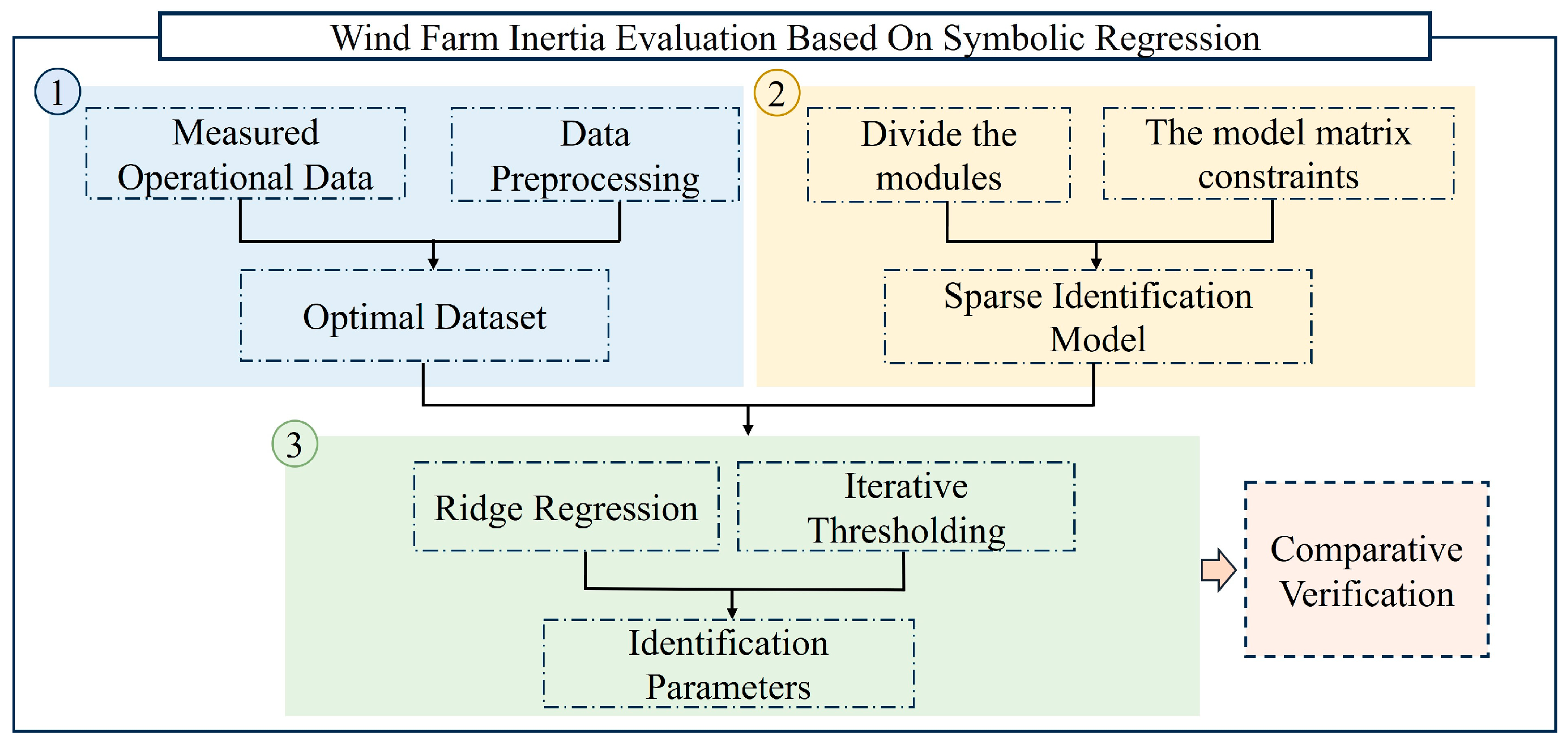
The proposed sparse dynamic modeling method divides the DFIG control modules and constructs input–output nonlinear feature libraries based on prior knowledge. The SR3 identification algorithm is used to estimate the model parameters. The simulation results validate the method’s effectiveness in evaluating the equivalent virtual inertia of wind farms in the IEEE three-machine nine-bus system, proving its feasibility and accuracy.

(3)

Compared to existing methods, the method proposed in this paper is capable of handling partially known or structurally opaque control components, which is critical in practical wind turbine systems, particularly when control structures and parameters are unknown or subject to commercial confidentiality constraints. The identified models retain a symbolic, interpretable form, unlike black-box neural networks. The sparse formulation promotes the compactness and physical relevance of the derived models.

Future work will focus on extending the proposed method to larger and more complex power systems, particularly heterogeneous renewable energy systems, in order to assess their inertia characteristics and frequency support capabilities, thereby contributing to the stability and security of emerging grid environments. Moreover, in response to the structural diversity of control strategies used in real-world wind power applications, the framework will be further applied for its applicability to other forms of inertia control, such as adaptive inertia control, coordinated synthetic inertia, manufacturer-specific variants and so on.

References

1. Yang, D.; Wang, X.; Chen, W.; Yan, G.-G.; Jin, Z.; Jin, E.; Zheng, T. Adaptive Frequency Droop Feedback Control-Based Power Tracking Operation of a DFIG for Temporary Frequency Regulation. IEEE Trans. Power Syst. 2023, 39, 2682–2692. [Google Scholar] [CrossRef]
2. Zhou, Y.; Zhu, D.; Zou, X.; He, C.; Hu, J.; Kang, Y. Adaptive Temporary Frequency Support for DFIG-Based Wind Turbines. IEEE Trans. Energy Convers. 2023, 38, 1937–1949. [Google Scholar] [CrossRef]
3. Cheng, H.; Li, C.; Ghias, A.M.Y.M.; Blaabjerg, F. Dynamic Coupling Mechanism Analysis Between Voltage and Frequency in Virtual Synchronous Generator System. IEEE Trans. Power Syst. 2023, 39, 2365–2368. [Google Scholar] [CrossRef]
4. Ochoa, D.; Martinez, S. Fast-Frequency Response Provided by DFIG-Wind Turbines and its Impact on the Grid. IEEE Trans. Power Syst. 2016, 32, 4002–4011. [Google Scholar] [CrossRef]
5. Yan, W.; Wang, X.; Gao, W.; Gevorgian, V. Electro-mechanical Modeling of Wind Turbine and Energy Storage Systems with Enhanced Inertial Response. J. Mod. Power Syst. Clean. Energy 2020, 8, 820–830. [Google Scholar] [CrossRef]
6. Abouyehia, M.; Egea-Àlvarez, A.; Ahmed, K.H. Evaluating inertia estimation methods in low-inertia power systems: A comprehensive review with analytic hierarchy process-based ranking. Renew. Sustain. Energy Rev. 2025, 217, 115794. [Google Scholar] [CrossRef]
7. Sun, L.; Zhao, X. Impacts of Phase-Locked Loop and Reactive Power Control on Inertia Provision by DFIG Wind Turbine. IEEE Trans. Energy Convers. 2022, 37, 109–119. [Google Scholar] [CrossRef]
8. Australian Energy Market Commission. Mechanisms to Enhance Resilience in the Power System—Review of the South Australian Black System Event. [2023-03-21]. Available online: https://www.aemc.gov.au/sites/default/files/documents/aemc_-_sa_black_system_review_-_final_report.pdf (accessed on 31 August 2019).
9. Ruifeng, Y. The anatomy of the 2016 South Australia blackout: A catastrophic event in a high renewable network. IEEE Trans. Power Syst. 2018, 33, 5374–5388. [Google Scholar] [CrossRef]
10. National Grid ESO. Technical Report on the Events of 9 August 2019; National Grid ESO: Warwick, UK, 2019. [Google Scholar]
11. Miller, N.W.; Price, W.W.; Sanchez-Gasca, J.J. Dynamic Modeling of GE 1.5 and 3.6 Wind Turbine-Generators: GE-Power Systems Energy Consulting, 2003; Power Engineering Society General Meeting: Toronto, ON, Canada, 2003; pp. 1977–1983. [Google Scholar]
12. Zhao, J.; Gómez-Expósito, A.; Netto, M.; Mili, L.; Abur, A.; Terzija, V.; Kamwa, I.; Pal, B.; Singh, A.K.; Qi, J.; et al. Power System Dynamic State Estimation: Motivations, Definitions, Methodologies, and Future Work. IEEE Trans. Power Syst. 2019, 34, 3188–3198. [Google Scholar] [CrossRef]
13. Ratnam, K.S.; Palanisamy, K.; Yang, G. Future low-inertia power systems: Requirements, issues, and solutions—A review. Renew. Sustain. Energy Rev. 2020, 124, 109773. [Google Scholar] [CrossRef]
14. Makolo, P.; Zamora, R.; Lie, T.-T. The role of inertia for grid flexibility under high penetration of variable renewables—A review of challenges and solutions. Renew. Sustain. Energy Rev. 2021, 147, 111223. [Google Scholar] [CrossRef]
15. Qi, Y.; Deng, H.; Liu, X.; Tang, Y. Synthetic Inertia Control of Grid-Connected Inverter Considering the Synchronization Dynamics. IEEE Trans. Power Electron. 2022, 37, 1411–1421. [Google Scholar] [CrossRef]
16. Berizzi, A.; Bosisio, A.; Ilea, V.; Marchesini, D.; Perini, R.; Vicario, A. Analysis of Synthetic Inertia Strategies from Wind Turbines for Large System Stability. IEEE Trans. Ind. Appl. 2022, 58, 3184–3192. [Google Scholar] [CrossRef]
17. Fernández-Guillamón, A.; Gómez-Lázaro, E.; Muljadi, E.; Molina-García, Á. Power systems with high renewable energy sources: A review of inertia and frequency control strategies over time. Renew. Sustain. Energy Rev. 2019, 115, 109369. [Google Scholar] [CrossRef]
18. Wu, Z.; Gao, W.; Gao, T.; Yan, W.; Zhang, H.; Yan, S.; Wang, X. State-of-the-art review on frequency response of wind power plants in power systems. J. Mod. Power Syst. Clean. Energy 2018, 6, 1–16. [Google Scholar] [CrossRef]
19. Chen, W.; Zheng, T.; Nian, H.; Yang, D.; Yang, W.; Geng, H. Multi-Objective Adaptive Inertia and Droop Control Method of Wind Turbine Generators. IEEE Trans. Ind. Appl. 2023, 59, 7789–7799. [Google Scholar] [CrossRef]
20. Sun, H.D.; Wang, B.C.; Li, W.F.; Yang, C.; Wei, W.; Zhao, B. Research on Inertia System of Frequency Response for Power System with High Penetration Electronics. Proc. CSEE 2020, 40, 5179–5191. [Google Scholar]
21. Lu, Z.; Jiang, J.; Qiao, Y.; Min, Y.; Li, H. A Review on Generalized Inertia Analysis and Optimization of New Power Systems. Proc. CSEE 2023, 43, 1754–1776. [Google Scholar]
22. Hosseini, S.A.; Fotuhi-Firuzabad, M.; Dehghanian, P.; Lehtonen, M. Coordinating Demand Response and Wind Turbine Controls for Alleviating the First and Second Frequency Dips in Wind-Integrated Power Grids. IEEE Trans. Ind. Inform. 2023, 20, 2223–2233. [Google Scholar] [CrossRef]
23. Ye, Y.; Qiao, Y.; Lu, Z. Revolution of frequency regulation in the converter-dominated power system. Renew. Sustain. Energy Rev. 2019, 111, 145–156. [Google Scholar] [CrossRef]
24. He, W.; Yuan, X.; Hu, J. Inertia provision and estimation of PLL-based DFIG wind turbines. IEEE Trans. Power Syst. 2017, 32, 510–521. [Google Scholar] [CrossRef]
25. Tian, X.; Wang, W.; Chi, Y.; Li, Y.; Liu, C. Virtual inertia optimization control of DFIG and assessment of equivalent inertia time constant of power grid. IET Renew. Poer Gener. 2018, 12, 1733–1740. [Google Scholar] [CrossRef]
26. Zhang, Y.; Bank, J.; Wan, Y.H.; Muljadi, E.; Corbus, D. Synchrophasor measurement-based wind plant inertia estimation. In Proceedings of the 2013 IEEE Green Technologies Conference, Denver, CO, USA, 4–5 April 2013; pp. 494–499. [Google Scholar]
27. Paidi, E.S.N.R.; Marzooghi, H.; Yu, J.; Terzija, V. Development and validation of artificial neural network-based tools for forecasting of power system inertia with wind farms penetration. IEEE Syst. J. 2020, 14, 4978–4989. [Google Scholar] [CrossRef]
28. Cao, X.; Stephen, B.; Abdulhadi, I.F.; Booth, C.D.; Burt, G.M. Switching Markov Gaussian Models for Dynamic Power System Inertia Estimation. IEEE Trans. Power Syst. 2016, 31, 3394–3403. [Google Scholar] [CrossRef]
29. Xing, Q.; Wang, T.; Huang, S. On-line identification of equivalent inertia for DFIG wind turbines based on extended Kalman filters. In Proceedings of the 2021 IEEE/IAS Industrial and Commercial Power System Asia (I&CPS Asia), Chengdu, China, 18–21 July 2021; pp. 834–839. [Google Scholar]
30. Wu, Y.; Zhao, X.; Shao, J.; Chen, X.; Yuan, J.; Wang, J. Inertia Estimation for Microgrid Considering the Impact of Wind Conditions on Doubly-Fed Induction Generators. IEEE Trans. Sustain. Energy 2024, 15, 2115–2125. [Google Scholar] [CrossRef]
31. Zhu, J.; Guo, L.; Wang, W.; Chen, B.; Yu, L.; Xu, S.; Jia, H. Temporal Spatio Inertia Perception of Global Power Grid Based on Adaptive Variable-order Fitting of Second-order Penalty Function. Autom. Electr. Power Syst. 2024, 48, 69–79. [Google Scholar]
32. Li, S.; Deng, C.; Long, Z.; Zhou, Q.; Zheng, F. Calculation of Equivalent Virtual Inertia Time Constant of Wind Farms. Autom. Electr. Power Syst. 2016, 40, 22–29. [Google Scholar]
33. Guo, J.; Wang, X.; Ooi, B.T. Estimation of Inertia for Synchronous and Non-Synchronous Generators Based on Ambient Measurements. IEEE Trans. Power Syst. 2022, 37, 3747–3757. [Google Scholar] [CrossRef]
34. Tuttelberg, K.; Kilter, J.; Wilson, D.H.; Uhlen, K. Estimation of Power System Inertia From Ambient Wide Area Measurements. IEEE Trans. Power Syst. 2018, 33, 7249–7257. [Google Scholar] [CrossRef]
35. Zeng, F.; Zhang, J.; Chen, G.; Wu, Z.; Huang, S.; Liang, Y. Online estimation of power system inertia constant under normal operating conditions. IEEE Access 2020, 8, 101426–101436. [Google Scholar] [CrossRef]
36. Qi, Y.; Yang, T.; Fang, J.; Tang, Y.; Potti, K.R.R.; Rajashekara, K. Grid Inertia Support Enabled by Smart Loads. IEEE Trans. Power Electron. 2020, 36, 947–957. [Google Scholar] [CrossRef]
37. Dreidy, M.; Mokhlis, H.; Mekhilef, S. Inertia response and frequency control techniques for renewable energy sources: A review. Renew. Sustain. Energy Rev. 2017, 69, 144–155. [Google Scholar] [CrossRef]
38. Mauricio, J.M.; Marano, A.; Gomez-Exposito, A.; Ramos, J.L.M. Frequency Regulation Contribution Through Variable-Speed Wind Energy Conversion Systems. IEEE Trans. Power Syst. 2009, 24, 173–180. [Google Scholar] [CrossRef]
39. Wang, T.; Xing, Q.; Li, H. Online evaluation and response characteristics analysis of equivalent inertia of a doubly-fed induction generator incorporating virtual inertia control. Prot. Control. Mod. Power Syst. 2022, 50, 52–60. [Google Scholar]
40. Li, H.; Zhang, X.; Wang, Y.; Zhu, X. Virtual inertia control of DFIG-based wind turbines based on the optimal power tracking. Proceeding CSEE 2012, 32, 32–39. [Google Scholar]
41. Liu, H.M.; Ren, Q.Y.; Zhang, Z.K.; Li, Y. Calculation of Equivalent Inertial Time Constant for Doubly-fed Induction Generators and Slip-feedback Inertia Control Strategy. Autom. Electr. Power Syst. 2018, 42, 49–57. [Google Scholar]
42. Champion, K.; Zheng, P.; Aravkin, A.Y.; Brunton, S.L.; Kutz, J.N. A Unified Sparse Optimization Framework to Learn Parsimonious Physics-Informed Models From Data. IEEE Access 2020, 8, 169259–169271. [Google Scholar] [CrossRef]
43. Loiseau, J.-C.; Brunton, S.L. Constrained sparse Galerkin regression. J. Fluid Mech. 2018, 838, 42–67. [Google Scholar] [CrossRef]
44. Zheng, P.; Askham, T.; Brunton, S.L.; Kutz, J.N.; Aravkin, A.Y. A Unified Framework for Sparse Relaxed Regularized Regression: SR3. IEEE Access 2018, 7, 1404–1423. [Google Scholar] [CrossRef]
45. Liu, J.; Wang, C.; Zhao, J.; Tan, B.; Bi, T. Simplified Transient Model of DFIG Wind Turbine for COI Frequency Dynamics and Frequency Spatial Variation Analysis. IEEE Trans. Power Syst. 2023, 39, 3752–3768. [Google Scholar] [CrossRef]
46. Jun, A.N.; Shuai, S.; Yibo, Z. Evaluation of equivalent virtual inertia of wind farm based on measured data. Power Syst. Technol. 2023, 47, 1819–1829. [Google Scholar]
47. Zhou, T.; Huang, J.; Han, R.S. Inertial Support Capacity Analysis and Equivalent Inertia Estimation of Wind Turbines Under Integrated Inertial Control. J. Shanghai Jiaotong Univ. 2024, 58, 1–24. [Google Scholar]
Figure 1. Inertial control model of DFIG.
Applsci 15 08578 g001
Figure 2. Matrix characterization of model constraints.
Applsci 15 08578 g002
Figure 3. Identification and validation path.
Applsci 15 08578 g003
Figure 4. IEEE three-machine nine-bus standard system.
Applsci 15 08578 g004
Figure 5. Partial identification of data acquisition: (a) grid angular frequency operating data; (b) power of inertia control operating date.
Applsci 15 08578 g005
Figure 6. Simulated and evaluated inertia values at different inertia control.
Applsci 15 08578 g006
Figure 7. Partial identification of data acquisition: (a) rotor speed operating data; (b) grid angular frequency operating data; (c) power of inertia control operating date.
Applsci 15 08578 g007
Figure 8. Simulated and evaluated inertia values at different wind speeds.
Applsci 15 08578 g008
Figure 9. Simulated and evaluated inertia values at different Kp levels.
Applsci 15 08578 g009
Figure 10. Simulated and evaluated inertia values at different Kd2 levels.
Applsci 15 08578 g010
Figure 11. Simulated and evaluated inertia values at different Tf levels.
Applsci 15 08578 g011