Figure 1.
Schematic x–t diagram illustrating stress wave propagation and spall phenomenon: (C) incident compressive wave, (T) reflected tensile wave, and the spall event. Unloading waves are generated from the spall plane.
Figure 1.
Schematic x–t diagram illustrating stress wave propagation and spall phenomenon: (C) incident compressive wave, (T) reflected tensile wave, and the spall event. Unloading waves are generated from the spall plane.
Figure 2.
Typical free surface velocity history illustrating the peak velocity (), rebound velocity (), and the calculation of the pull-back velocity ().
Figure 2.
Typical free surface velocity history illustrating the peak velocity (), rebound velocity (), and the calculation of the pull-back velocity ().
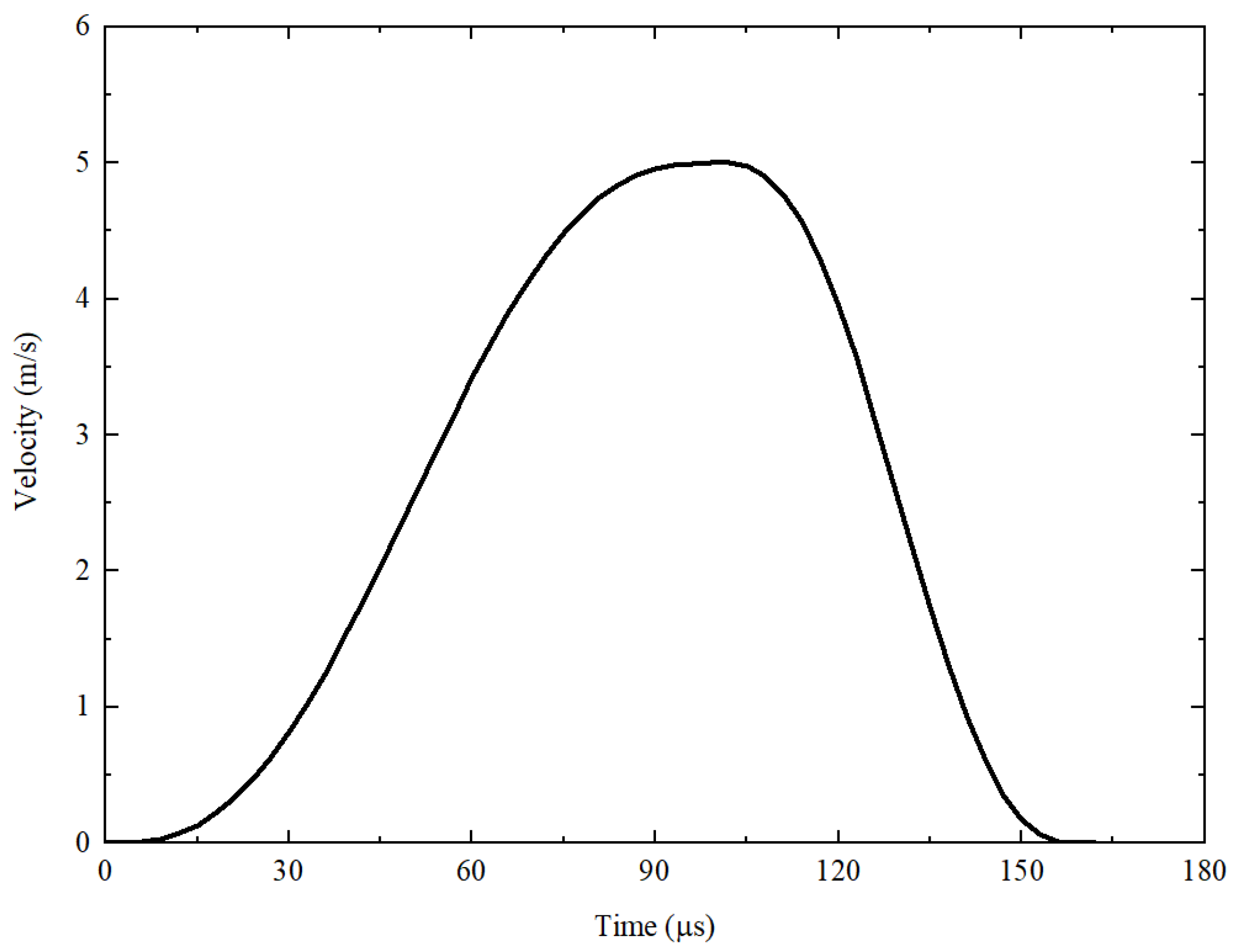
Figure 3.
Prescribed velocity history applied as the input boundary condition at the left end of the FEM specimen model.
Figure 3.
Prescribed velocity history applied as the input boundary condition at the left end of the FEM specimen model.
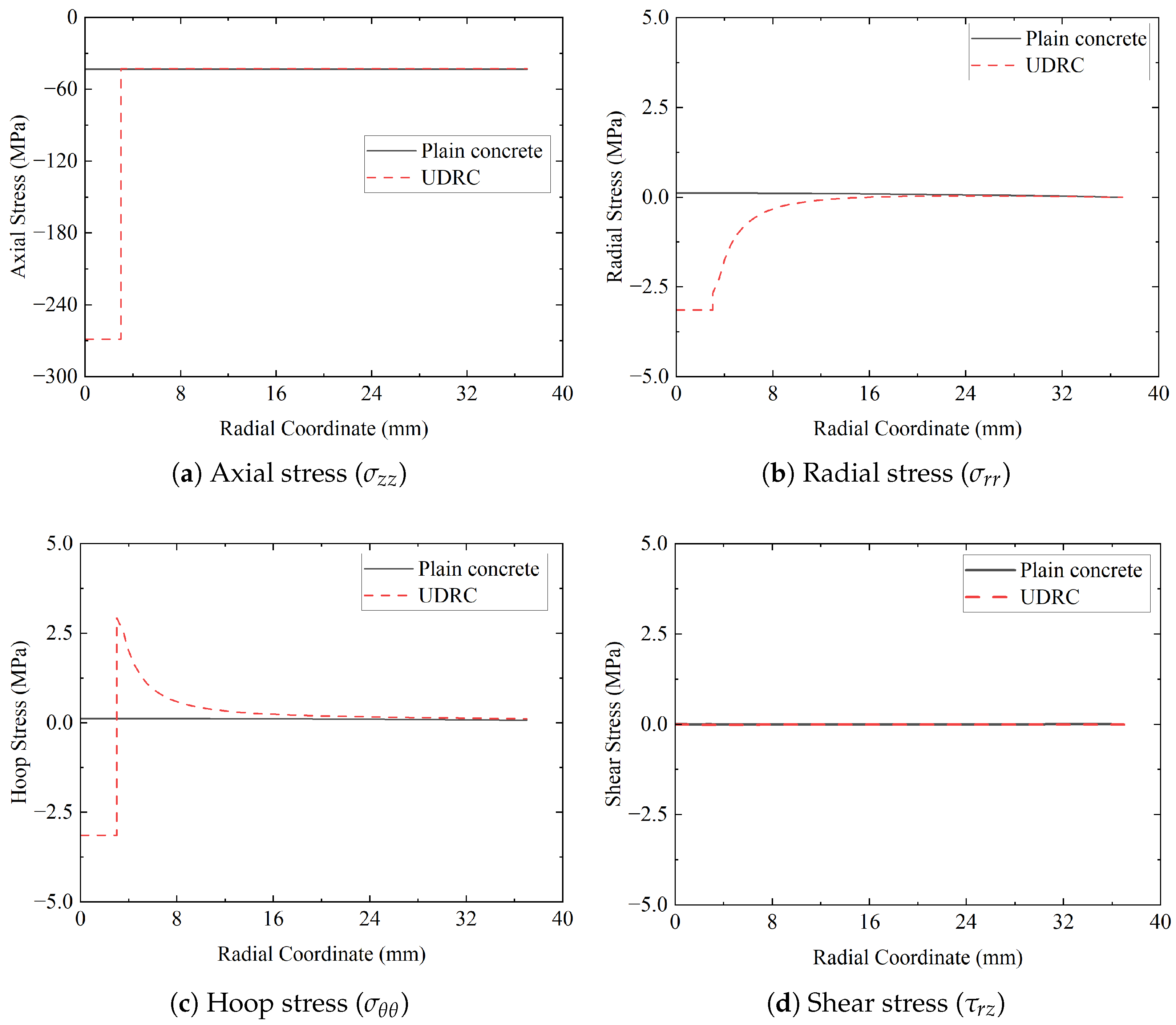
Figure 4.
Comparison of radial distribution of stress components between UDRC and plain concrete (PC) specimens at the cross-section 535.5 mm from the impact end (at time of peak axial compression): (a) axial stress, (b) radial stress, (c) hoop stress, and (d) shear stress .
Figure 4.
Comparison of radial distribution of stress components between UDRC and plain concrete (PC) specimens at the cross-section 535.5 mm from the impact end (at time of peak axial compression): (a) axial stress, (b) radial stress, (c) hoop stress, and (d) shear stress .
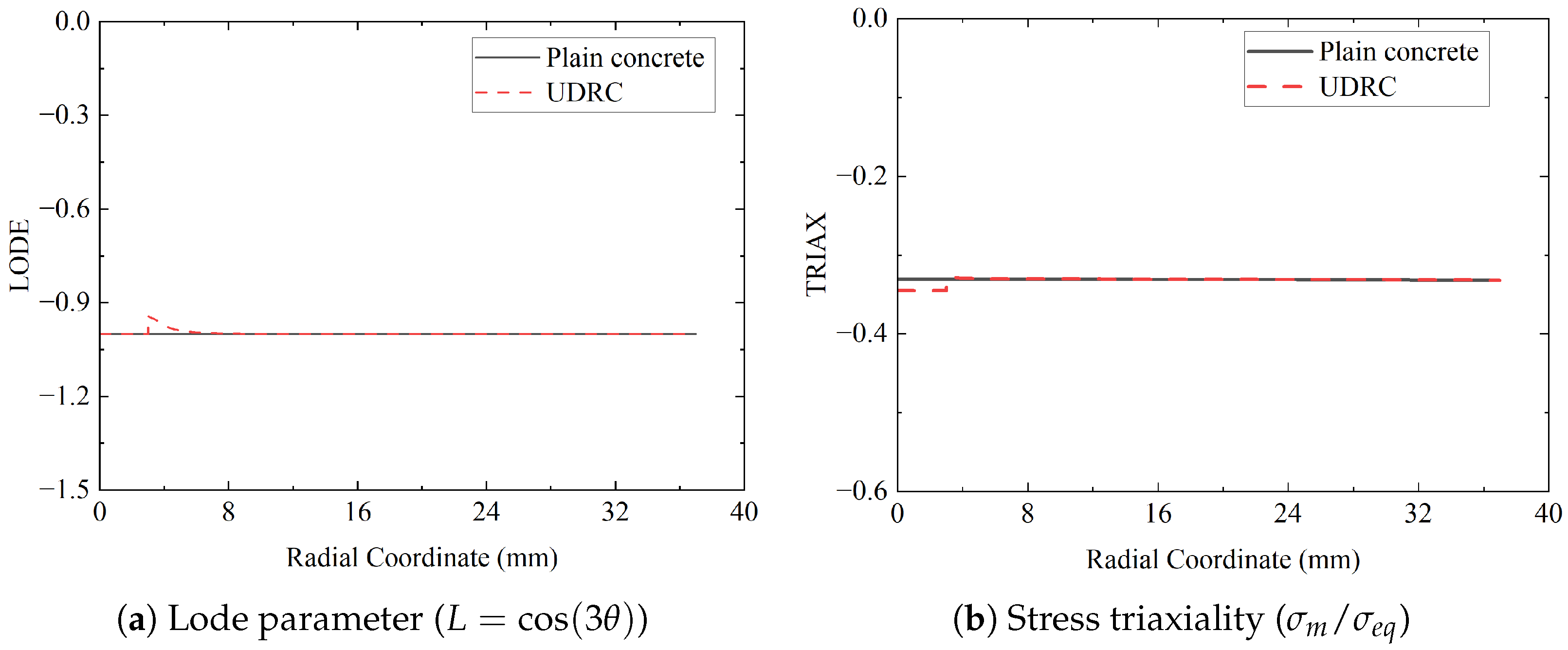
Figure 5.
Comparison of radial distribution of (a) Lode parameter and (b) stress triaxiality between UDRC and plain concrete (PC) specimens at the cross-section 535.5 mm from the impact end (at time of peak axial compression).
Figure 5.
Comparison of radial distribution of (a) Lode parameter and (b) stress triaxiality between UDRC and plain concrete (PC) specimens at the cross-section 535.5 mm from the impact end (at time of peak axial compression).
Figure 6.
Radial distribution of stress components in a UDRC specimen at the time and location just prior to the initiation of tensile spall fracture.
Figure 6.
Radial distribution of stress components in a UDRC specimen at the time and location just prior to the initiation of tensile spall fracture.
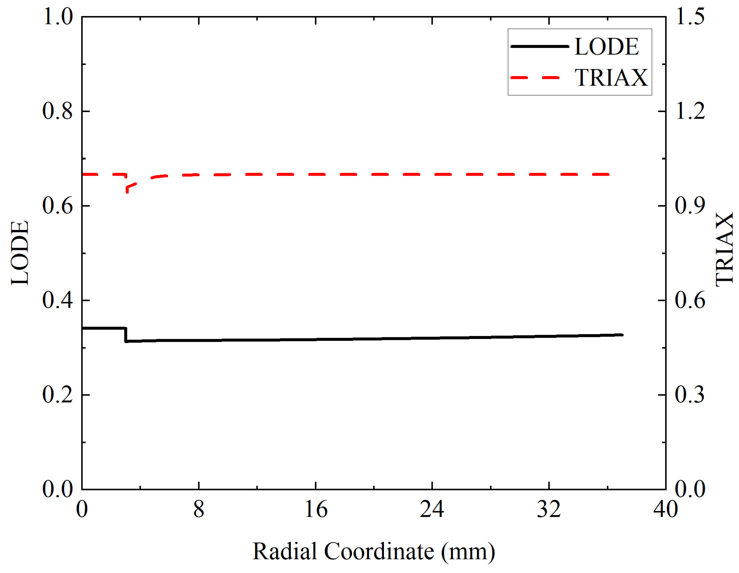
Figure 7.
Radial distribution of the stress triaxiality and Lode parameter in a UDRC specimen at the time and location just prior to the initiation of tensile spall fracture.
Figure 7.
Radial distribution of the stress triaxiality and Lode parameter in a UDRC specimen at the time and location just prior to the initiation of tensile spall fracture.
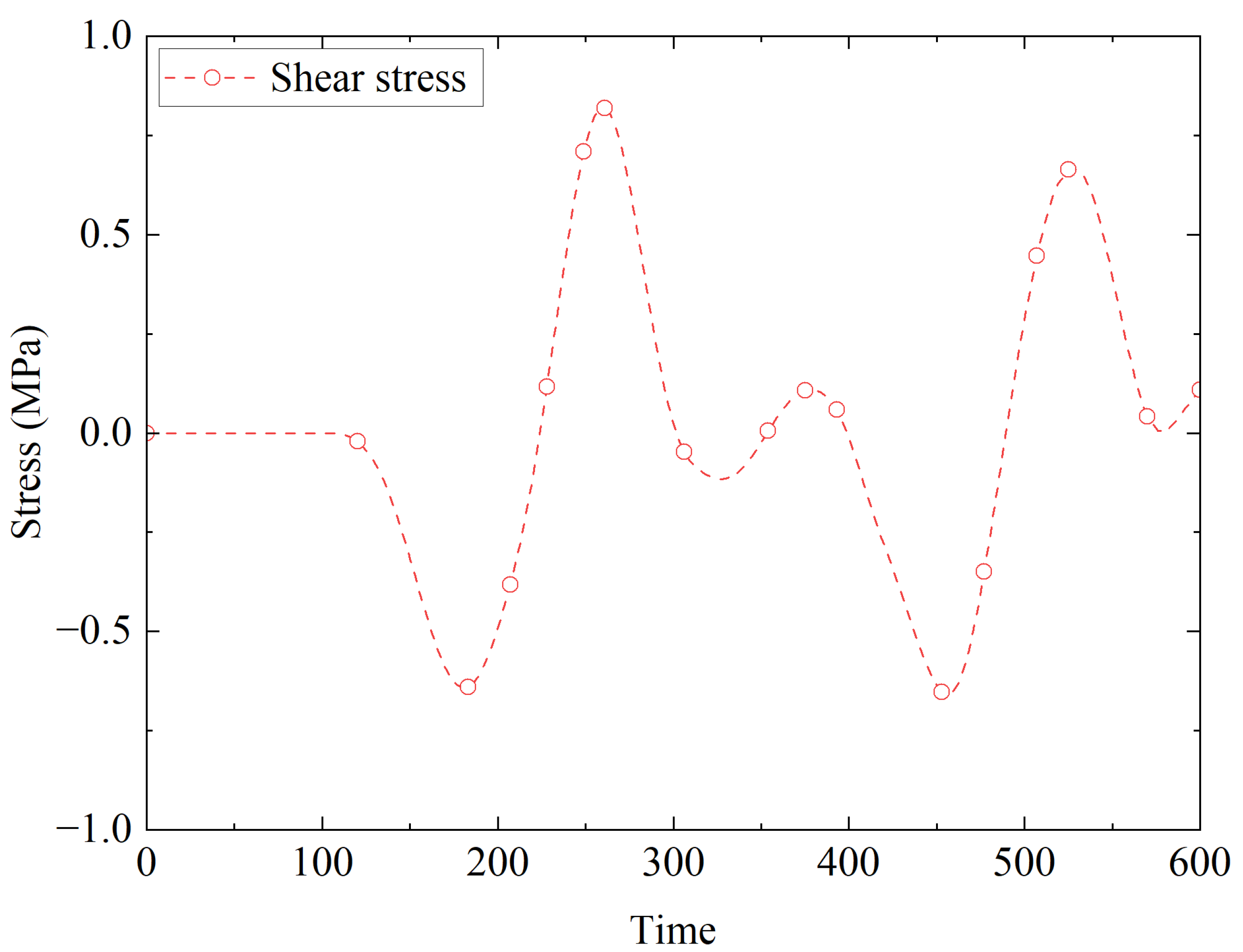
Figure 8.
Temporal evolution of interface shear stress at the steel–concrete interface. The peak stress of MPa remains significantly below the theoretical bond failure threshold of MPa.
Figure 8.
Temporal evolution of interface shear stress at the steel–concrete interface. The peak stress of MPa remains significantly below the theoretical bond failure threshold of MPa.
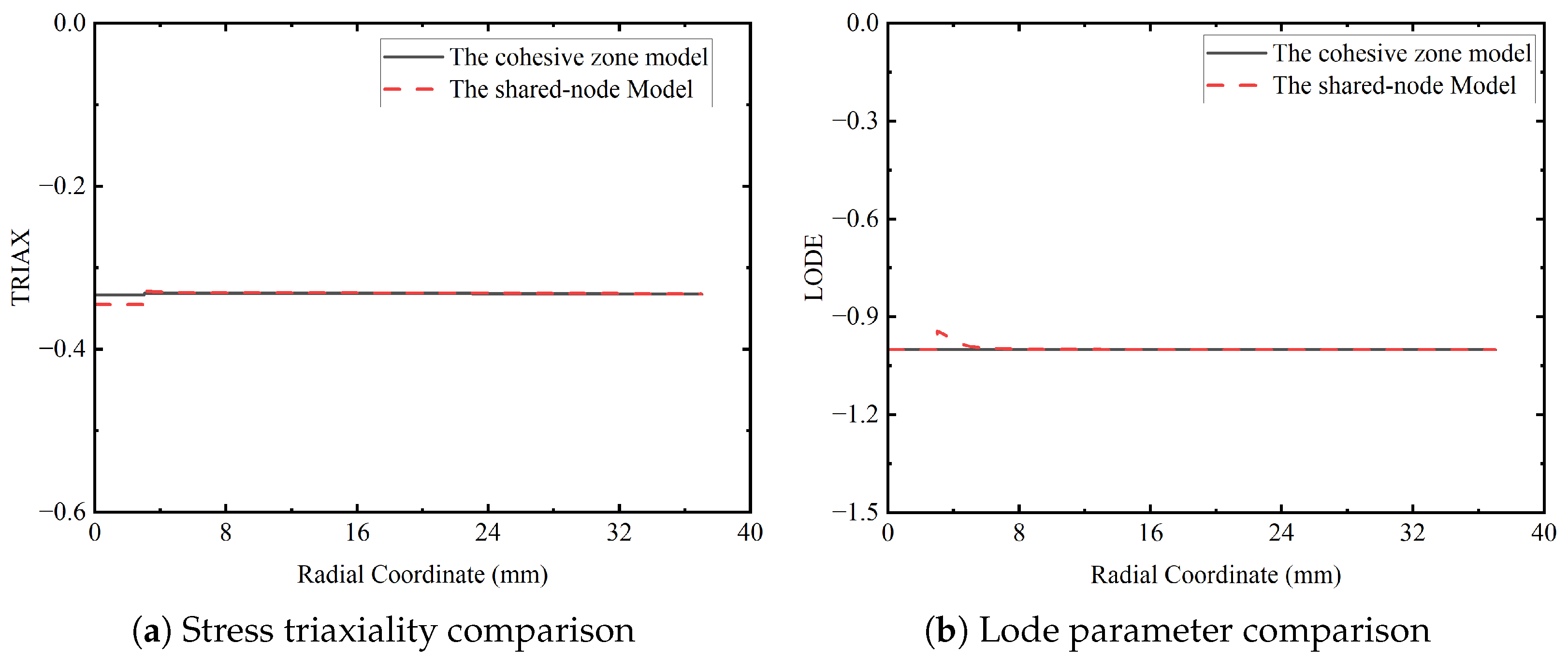
Figure 9.
Comparison of (a) stress triaxiality and (b) Lode parameter distributions between shared-node and cohesive zone models at the cross-section 535.5 mm from the impact end, demonstrating improved uniaxial stress conditions with cohesive modeling.
Figure 9.
Comparison of (a) stress triaxiality and (b) Lode parameter distributions between shared-node and cohesive zone models at the cross-section 535.5 mm from the impact end, demonstrating improved uniaxial stress conditions with cohesive modeling.
Figure 10.
Comparison of simulated free surface velocity histories for plain concrete and UDRC specimens (plain and deformed reinforcement) subjected to identical input loading.
Figure 10.
Comparison of simulated free surface velocity histories for plain concrete and UDRC specimens (plain and deformed reinforcement) subjected to identical input loading.
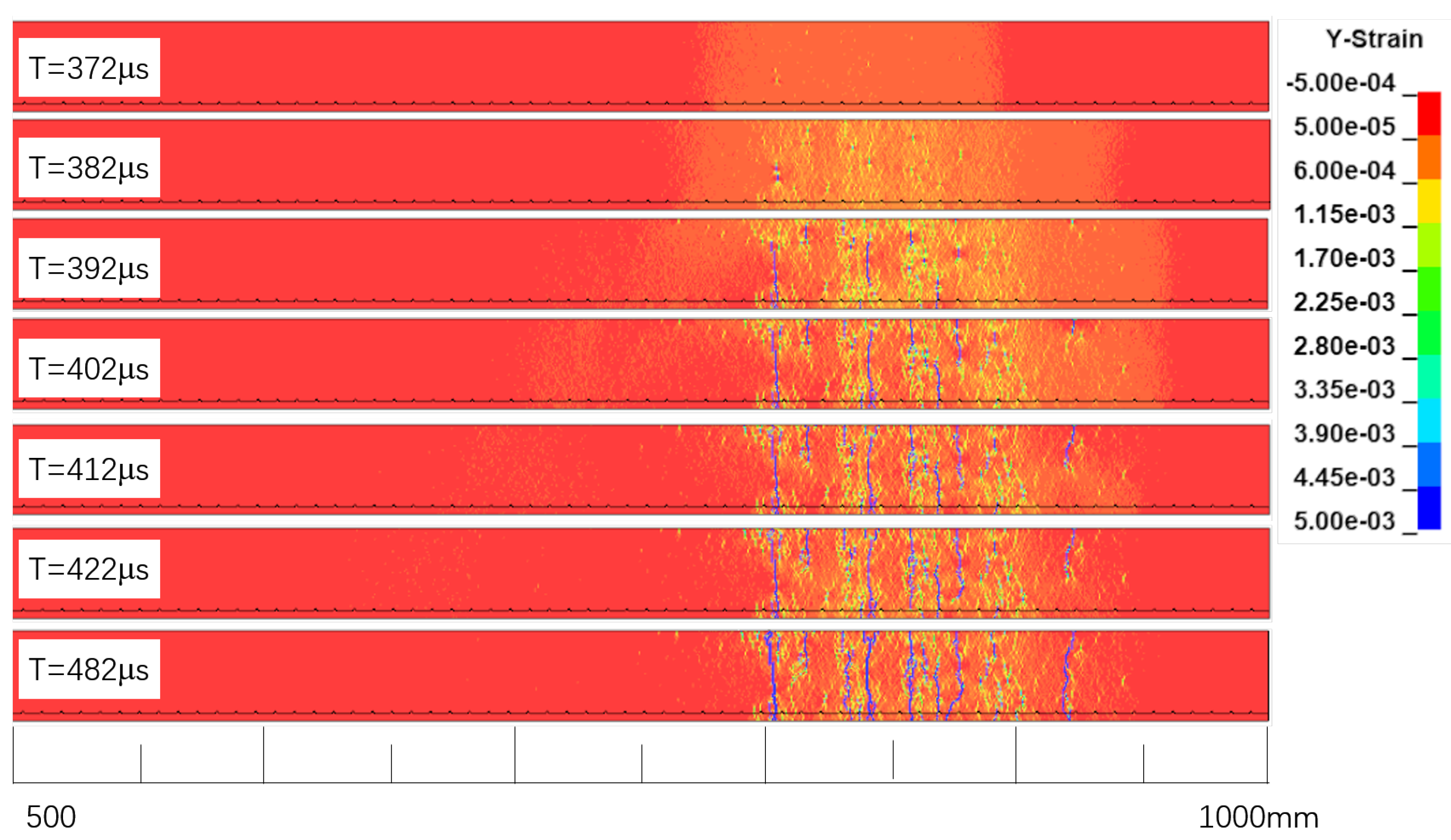
Figure 11.
Simulated strain field evolution and spall fracture process in a plain concrete specimen.
Figure 11.
Simulated strain field evolution and spall fracture process in a plain concrete specimen.
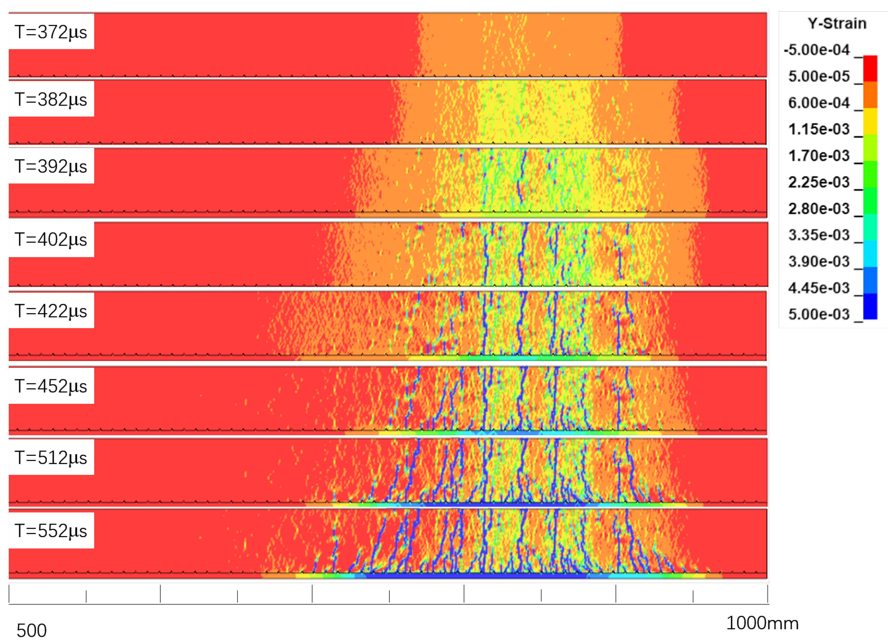
Figure 12.
Simulated strain field evolution and spall fracture process in a deformed UDRC specimen, showing the influence of reinforcement.
Figure 12.
Simulated strain field evolution and spall fracture process in a deformed UDRC specimen, showing the influence of reinforcement.
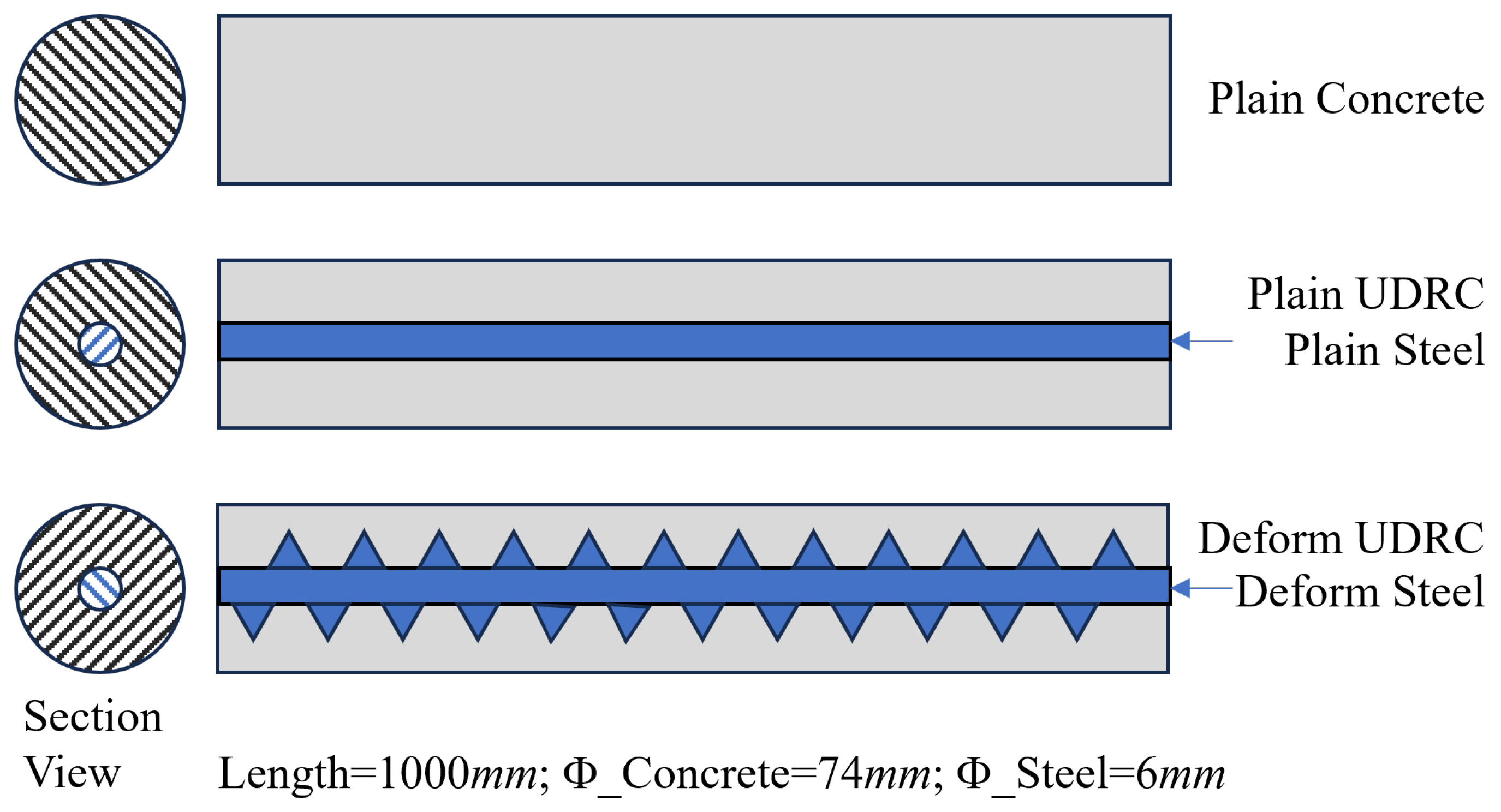
Figure 13.
Schematic diagram of the specimen types: (Top) Plain Concrete (PC), (Middle) Plain UDRC with a smooth steel bar, and (Bottom) Deformed UDRC with a ribbed steel bar.
Figure 13.
Schematic diagram of the specimen types: (Top) Plain Concrete (PC), (Middle) Plain UDRC with a smooth steel bar, and (Bottom) Deformed UDRC with a ribbed steel bar.
Figure 14.
Schematic of the SHPB experimental setup configured for one-dimensional spalling tests on concrete and UDRC specimens.
Figure 14.
Schematic of the SHPB experimental setup configured for one-dimensional spalling tests on concrete and UDRC specimens.
Figure 15.
Typical axial strain histories recorded by strain gauges on the specimen surface and the corresponding free-end surface velocity history measured by the laser vibrometer.
Figure 15.
Typical axial strain histories recorded by strain gauges on the specimen surface and the corresponding free-end surface velocity history measured by the laser vibrometer.
Figure 16.
Example of the artificial speckle pattern applied to the concrete specimen surface for DIC analysis.
Figure 16.
Example of the artificial speckle pattern applied to the concrete specimen surface for DIC analysis.
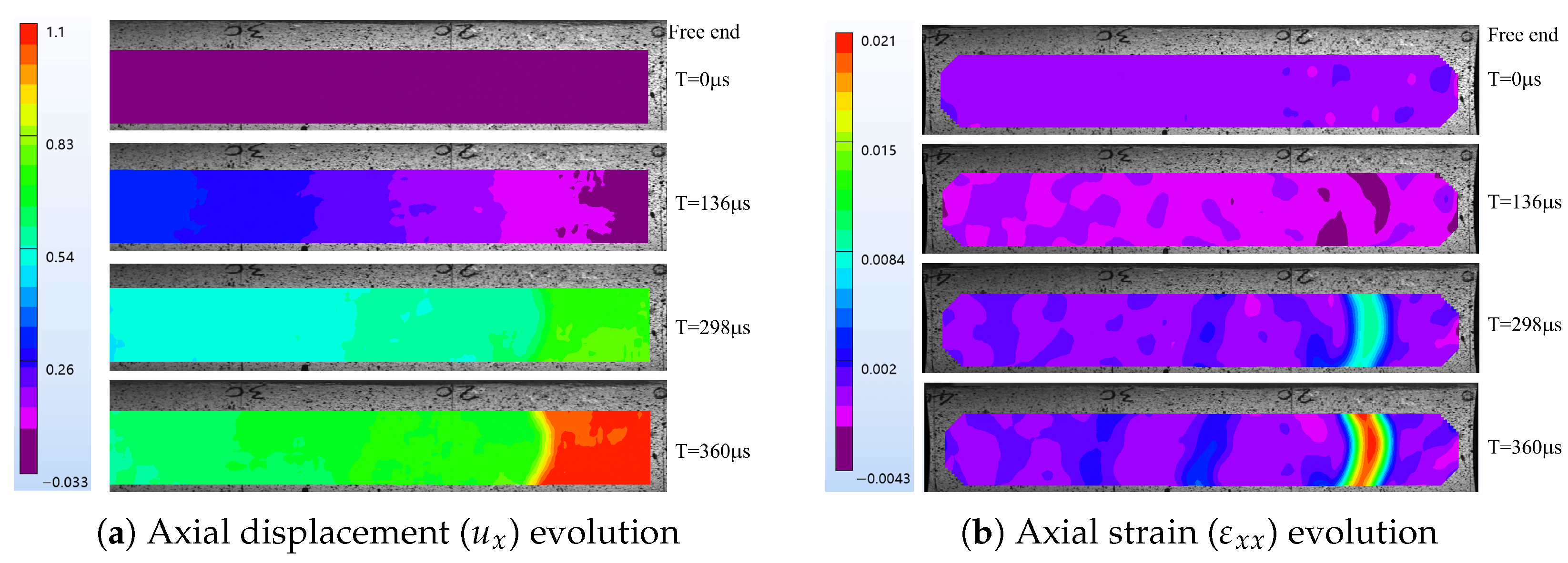
Figure 17.
DIC analysis for specimen Z003-25 showing the temporal evolution of (a) the axial displacement field and (b) the axial strain field. The images capture the wave propagation and subsequent strain localization leading to spall fracture near the free end.
Figure 17.
DIC analysis for specimen Z003-25 showing the temporal evolution of (a) the axial displacement field and (b) the axial strain field. The images capture the wave propagation and subsequent strain localization leading to spall fracture near the free end.
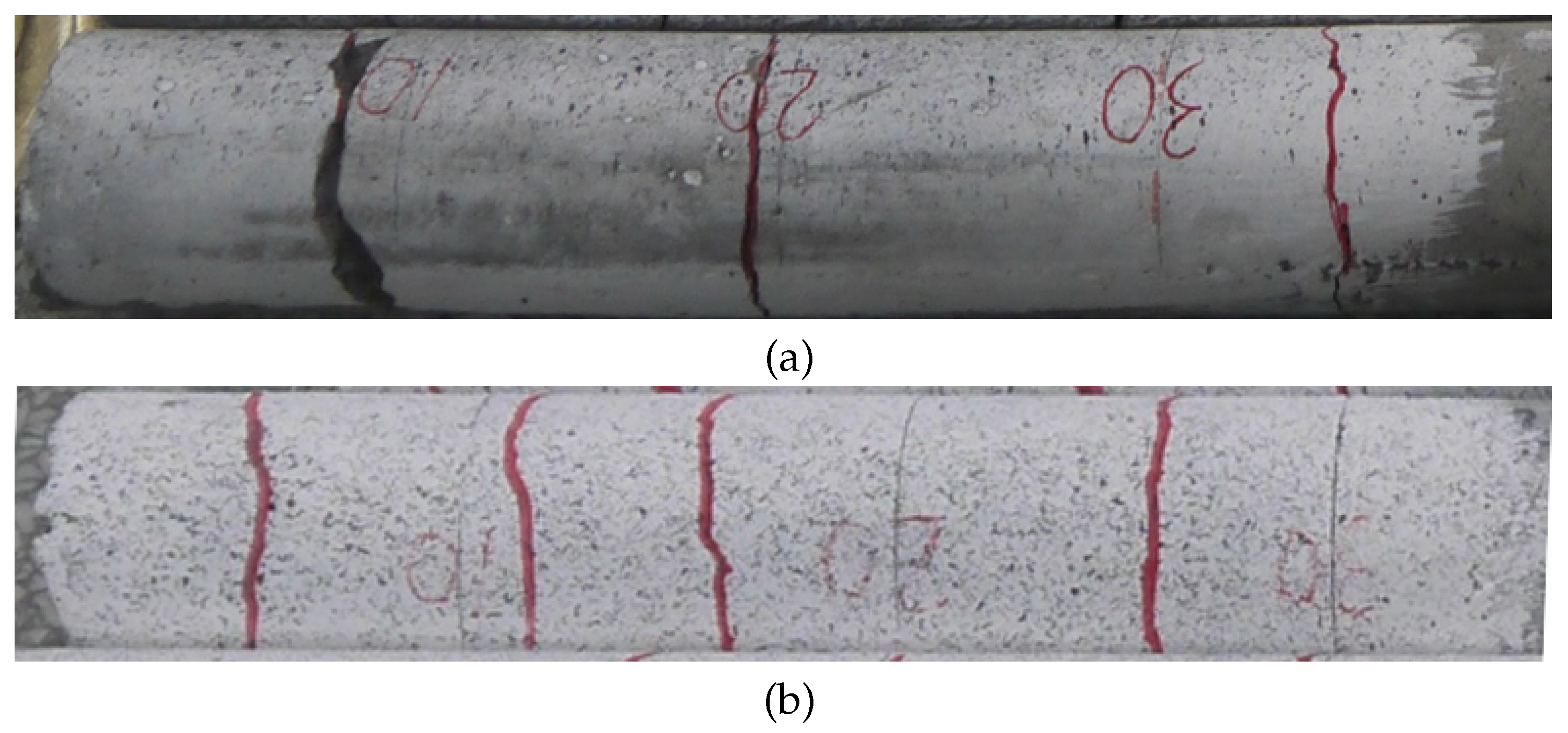
Figure 18.
Experimental comparison of post-spall failure modes from post-test photographs. (a) Three large, localized fractures in a plain concrete specimen, indicating imminent and complete separation. (b) Multiple (at least four) cracks in a deformed UDRC specimen which is held together by the central reinforcement, demonstrating the crack-bridging effect and maintenance of structural integrity.
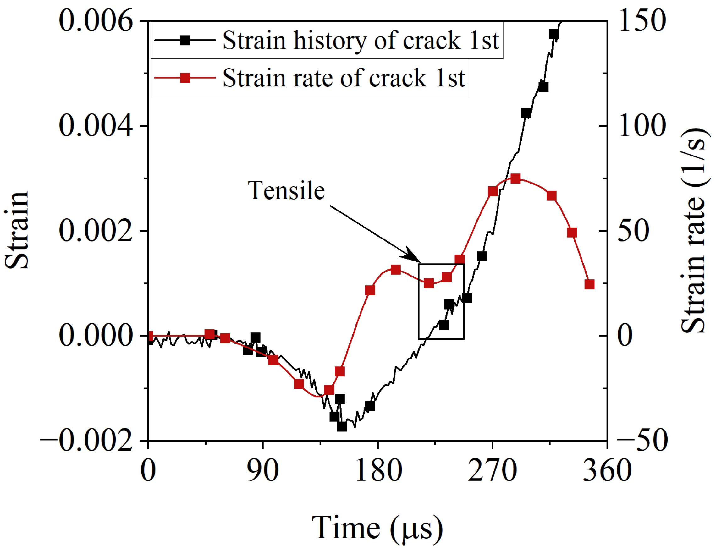
Figure 19.
Example of local axial strain history () and calculated strain rate history () at the primary spall crack location for specimen Z001-29.
Figure 19.
Example of local axial strain history () and calculated strain rate history () at the primary spall crack location for specimen Z001-29.
Figure 20.
Spall strength as a function of strain rate for all specimen types. The solid line represents the logarithmic fit to the combined dataset, with its equation and R-squared value shown.
Figure 20.
Spall strength as a function of strain rate for all specimen types. The solid line represents the logarithmic fit to the combined dataset, with its equation and R-squared value shown.
Table 1.
Material parameters for the concrete model.
Table 1.
Material parameters for the concrete model.
| Density (kg/m3) | Poisson’s Ratio | Tensile Strength/MPa | | | | | |
|---|
| 2379 | 0.2 | 4.6 | 1.6 | 5.5 | 1.15 | 0.5 | |
| | | | | | | |
| 22.38 | 0.463 | | 16.90 | 0.625 | | 0.4417 | |
| | | | | | | |
| 0 | | | | | | | |
| | | | | | | |
| | 1 | 10 | 100 | 0 | 0.85 | 0.97 |
| | | | | | | |
| 0.99 | 1 | 0.99 | 0.97 | 0.5 | 0.1 | 0 | 0 |
| | | | | | | |
| 0 | 0 | | | | | | |
Table 2.
Material parameters for the steel.
Table 2.
Material parameters for the steel.
| Elastic Modulus (GPa) | Poisson’s Ratio | Density (kg/m3) |
|---|
| 210 | 0.3 | 7800 |
Table 3.
Mix design of the C40 grade concrete.
Table 3.
Mix design of the C40 grade concrete.
| Component | Specification/Type |
|---|
| Cement | Haichang P.O 52.5 Portland cement |
| Admixture | CL-19 polycarboxylate superplasticizer |
| Supplementary Material | Class F Grade II fly ash |
| Fine Aggregate | Zone II medium sand |
| Coarse Aggregate | Continuously graded crushed stone (10 mm max. size) |
| Water-to-Cement Ratio | 0.5 |
Table 4.
Quasi-static mechanical properties of the C40 concrete *.
Table 4.
Quasi-static mechanical properties of the C40 concrete *.
| Density (kg/m3) | Young’s Modulus (GPa) | Poisson’s Ratio | Compressive Strength (MPa) | Tensile Strength (MPa) |
|---|
| 2379 | 32.0 | 0.20 | 60.0 | 4.6 |
Table 5.
Comprehensive experimental results from spalling tests, including local strain rates from DIC and calculated spall strengths and DIFs.
Table 5.
Comprehensive experimental results from spalling tests, including local strain rates from DIC and calculated spall strengths and DIFs.
| Test No. | Specimen Type | Test ID | Strain Rate (s−1) | Spall Strength (Mpa) | DIF |
|---|
| 1 | Plain Concrete | Z001-21 | 7.16 | 9.05 | 1.97 |
| 2 | Plain Concrete | Z001-13 | 11.80 | 10.72 | 2.33 |
| 3 | Plain Concrete | Z001-14 | 21.90 | 10.82 | 2.35 |
| 4 | Plain Concrete | Z001-29 | 25.00 | 9.74 | 2.12 |
| 5 | Plain Concrete | Z001-40 | 40.10 | 10.72 | 2.33 |
| 6 | Plain Concrete | Z001-30 | 54.70 | 12.11 | 2.63 |
| 7 | Plain UDRC | Z002-57 | 8.72 | 9.25 | 2.01 |
| 8 | Plain UDRC | Z002-10 | 13.00 | 8.71 | 1.89 |
| 9 | Plain UDRC | Z002-27 | 14.00 | 7.41 | 1.61 |
| 10 | Plain UDRC | Z002-05 | 15.10 | 10.35 | 2.25 |
| 11 | Plain UDRC | Z002-48 | 27.50 | 10.59 | 2.30 |
| 12 | Plain UDRC | Z002-06 | 34.40 | 13.59 | 2.95 |
| 13 | Deformed UDRC | Z003-49 | 2.96 | 6.70 | 1.46 |
| 14 | Deformed UDRC | Z003-15 | 5.74 | 6.40 | 1.39 |
| 15 | Deformed UDRC | Z003-28 | 9.02 | 8.22 | 1.79 |
| 16 | Deformed UDRC | Z003-20 | 14.40 | 9.64 | 2.10 |
| 17 | Deformed UDRC | Z003-25 | 22.60 | 7.30 | 1.59 |
| 18 | Deformed UDRC | Z003-38 | 30.00 | 9.47 | 2.06 |
Table 6.
Results of the analysis of covariance (ANCOVA) for spall strength.
Table 6.
Results of the analysis of covariance (ANCOVA) for spall strength.
| Source | Sum Sq. | d.f. | Mean Sq. | F | Prob > F |
|---|
| Specimen Type | 4.0661 | 2 | 2.0331 | 1.46 | 0.2701 |
| Log Strain Rate | 20.3741 | 1 | 20.3741 | 14.66 | 0.0024 |
| Specimen Type:Log Strain Rate | 4.8170 | 2 | 2.4085 | 1.73 | 0.2182 |
| Error | 16.6802 | 12 | 1.3900 | | |
| Total | 59.4312 | 17 | | | |


