
Application of Extra-Trees Regression and Tree-Structured Parzen Estimators Optimization Algorithm to Predict Blast-Induced Mean Fragmentation Size in Open-Pit Mines


Abstract
1. Introduction
2. Data Source
2.1. Data Collection and Supplement
2.2. Data Augmentation
3. Methodology
3.1. Random Forest Algorithm
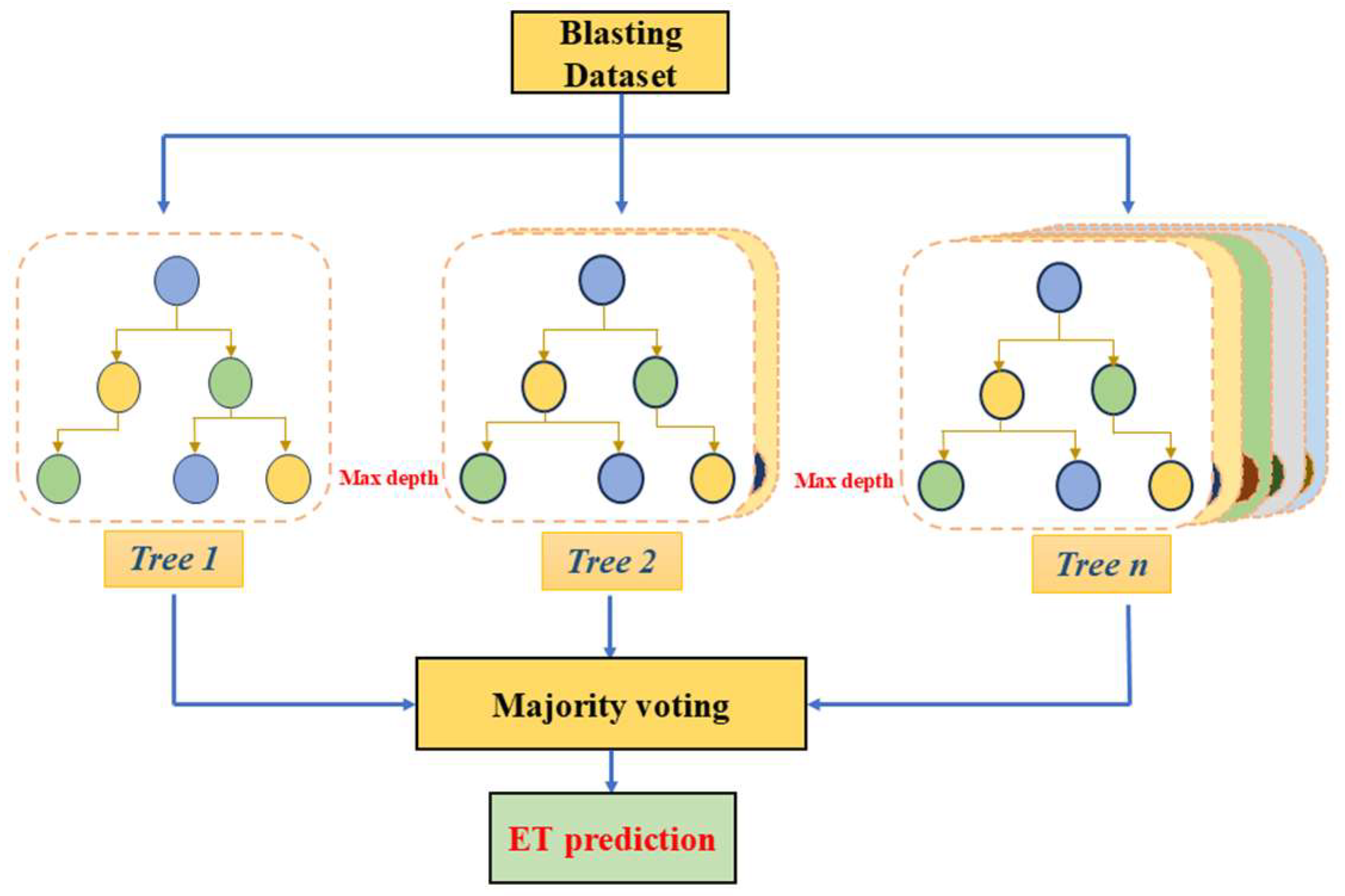
3.2. Extra Trees Algorithm
3.3. Gradient Boosting Algorithm
3.4. Optimization Algorithm: Bayesian Optimization
3.5. Shapley Additive Explanations for Model Interpretation
4. Model Development and Evaluation Indices
- (1)
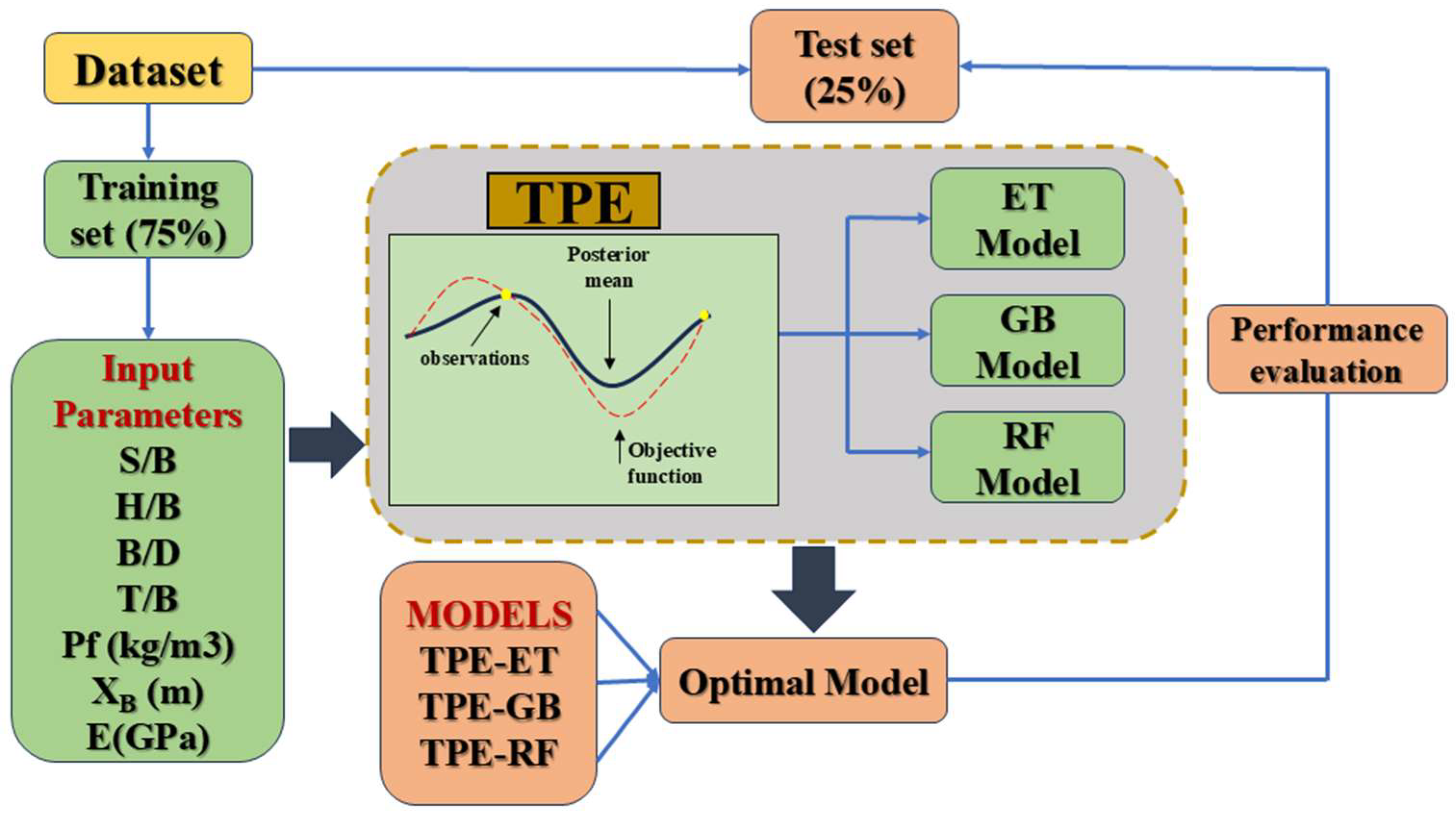
- Data preprocessing: The dataset is divided into training and test sets with 75% (2805 samples) being allocated for training and 25% (935 samples) being reserved for testing. This 75/25 data split was chosen for several reasons: (1) it provides enough samples for the models to learn patterns, which prevents underfitting; (2) smaller test sets tend to be biased while larger test sets offer a more representative sample; and (3) this split ratio generalizes better than a 70/30 split or 80/20 split. Figure 5 show the data distribution between the training and test datasets. It can be observed that the training and test sets are normally distributed; therefore, there is no need for further pre-processing. Additionally, the training and test sets are distributed the same;
- (2)
- Optimization process: Many influencing parameters can influence the performance of the algorithms, but only a limited number of hyperparameters were selected to balance performance and computational cost. Five hyperparameters were optimized for the RF and ET algorithms, while six were used for the GB algorithm, as shown in Table 4. These hyperparameters are critical for improving the accuracy of the models. The performance of the Bayesian optimization algorithm is influenced by the number of trials or iterations used to search for the optimal hyperparameter combinations. More trials result in longer training times and higher costs, whereas fewer trials may lead to underfitting. To maintain consistency across models, the number of trials was set to 150 for all models;
- (3)
- Model evaluation: In this study, four indices, including the root mean squared error (RMSE), mean absolute error (MAE), coefficient of determination (R2), and max error were employed to evaluate the performance of the three models. These metrics are described using Equations (15)–(18):


| Hyperparameters | Regression Algorithms Hyperparameter Search Spaces | Data Type | Description | ||
|---|---|---|---|---|---|
| TPE-ET | TPE-RF | TPE-GB | |||
| n estimators | [10, 3000] | [10, 3000] | [10, 3000] | Integer | Number of trees in the forest |
| max depth | [2, 40] | [2, 40] | [2, 40] | Integer | Maximum depth of each tree |
| min samples split | [2, 35] | [2, 35] | [2, 35] | Integer | The minimum number of samples required to split an internal code |
| criterion | ‘squared_error’, ‘absolute_error’, ‘friedman_mse’, ‘poisson’ | ‘squared_error’, ‘absolute_error’, ‘friedman_mse’, ‘poisson’ | ‘squared_error’, ‘friedman_mse’, | Categorical | These functions measure the quality of a split. |
| min impurity decrease | [0.00001, 0.9] | [0.00001, 0.9] | [0.00001, 0.9] | Float | It splits the node if the split induces a decrease of the impurity greater than or equal to this value. |
| learning rate | [0.00001, 0.9] | Float | It shrinks the contribution of each tree by the value of learning_rate. | ||
5. Results and Discussion
5.1. Performance Comparison of Models for MFS Prediction
5.2. Model Interpretation
6. Conclusions
- (1)
- Adding 3% noise to augment the dataset did not significantly distort the original dataset. Moreover, the large-scale database of 3740 samples provided deeper insights into the input and output parameters and thus enhanced the model’s predictive capabilities;
- (2)
- The model evaluation results demonstrated that the TPE-ET model performed better than the other models in predicting MFS, achieving R2, RMSE, MAE, and max error optimal values of 0.93, 0.04, 0.03, and 0.25 on the testing set;
- (3)
- The model interpretability results illustrated that rock parameters and geological conditions were the most significant parameters in predicting MFS. In this study, XB (m) and E (GPa) had the most significant impact and a positive contribution to the models’ predictions.
Author Contributions
Funding
Institutional Review Board Statement
Informed Consent Statement
Data Availability Statement
Acknowledgments
Conflicts of Interest
References
- Hu, H.; Lu, W.; Yan, P.; Chen, M.; Gao, Q.; Yang, Z. A new horizontal rock dam foundation blasting technique with a shock-reflection device arranged at the bottom of vertical borehole. Eur. J. Environ. Civ. Eng. 2020, 24, 481–499. [Google Scholar] [CrossRef]
- Zhou, J.; Chen, C.; Du, K.; Armaghani, D.J.; Li, C. A new hybrid model of information entropy and unascertained measurement with different membership functions for evaluating destressability in burst-prone underground mines. Eng. Comput. 2022, 38, 381–399. [Google Scholar] [CrossRef]
- Li, C.; Zhou, J. Prediction and optimization of adverse responses for a highway tunnel after blasting excavation using a novel hybrid multi-objective intelligent model. Transp. Geotech. 2024, 45, 101228. [Google Scholar] [CrossRef]
- Yang, Z.; He, B.; Liu, Y.; Wang, D.; Zhu, G. Classification of rock fragments produced by tunnel boring machine using convolutional neural networks. Autom. Constr. 2021, 125, 103612. [Google Scholar] [CrossRef]
- Ebrahimi, E.; Monjezi, M.; Khalesi, M.R.; Armaghani, D.J. Prediction and optimization of back-break and rock fragmentation using an artificial neural network and a bee colony algorithm. Bull. Eng. Geol. Environ. 2016, 75, 27–36. [Google Scholar] [CrossRef]
- Khandelwal, M.; Monjezi, M. Prediction of Backbreak in Open-Pit Blasting Operations Using the Machine Learning Method. Rock Mech. Rock Eng. 2013, 46, 389–396. [Google Scholar] [CrossRef]
- Monjezi, M.; Khoshalan, H.A.; Varjani, A.Y. Prediction of flyrock and backbreak in open pit blasting operation: A neuro-genetic approach. Arab. J. Geosci. 2012, 5, 441–448. [Google Scholar] [CrossRef]
- Esmaeili, M.; Osanloo, M.; Rashidinejad, F.; Bazzazi, A.A.; Taji, M. Multiple regression, ANN and ANFIS models for prediction of backbreak in the open pit blasting. Eng. Comput. 2014, 30, 549–558. [Google Scholar] [CrossRef]
- Zhou, J.; Asteris, P.G.; Armaghani, D.J.; Pham, B.T. Prediction of ground vibration induced by blasting operations through the use of the Bayesian Network and random forest models. Soil Dyn. Earthq. Eng. 2020, 139, 106390. [Google Scholar] [CrossRef]
- Armaghani, D.J.; Hajihassani, M.; Mohamad, E.T.; Marto, A.; Noorani, S.A. Blasting-induced flyrock and ground vibration prediction through an expert artificial neural network based on particle swarm optimization. Arab. J. Geosci. 2014, 7, 5383–5396. [Google Scholar] [CrossRef]
- Görgülü, K.; Arpaz, E.; Demirci, A.; Koçaslan, A.; Dilmaç, M.K.; Yüksek, A.G. Investigation of blast-induced ground vibrations in the Tülü boron open pit mine. Bull. Eng. Geol. Environ. 2013, 72, 555–564. [Google Scholar] [CrossRef]
- Raina, A.; Murthy, V.; Soni, A. Flyrock in bench blasting: A comprehensive review. Bull. Eng. Geol. Environ. 2014, 73, 1199–1209. [Google Scholar] [CrossRef]
- Jang, H.; Kitahara, I.; Kawamura, Y.; Endo, Y.; Topal, E.; Degawa, R.; Mazara, S. Development of 3D rock fragmentation measurement system using photogrammetry. Int. J. Min. Reclam. Environ. 2020, 34, 294–305. [Google Scholar] [CrossRef]
- Ouchterlony, F.; Sanchidrián, J.A. A review of the development of better prediction equations for blast fragmentation. Rock Dyn. Appl. 3 2018, 11, 25–45. [Google Scholar] [CrossRef]
- Zhang, Z.-X.; Hou, D.-F.; Guo, Z.; He, Z.; Zhang, Q. Experimental study of surface constraint effect on rock fragmentation by blasting. Int. J. Rock Mech. Min. Sci. 2020, 128, 104278. [Google Scholar] [CrossRef]
- Raina, A.K.; Vajre, R.; Sangode, A.; Chandar, K.R. Application of artificial intelligence in predicting rock fragmentation: A review. Appl. Artif. Intell. Min. Geotech. Geoengin. 2024, 291–314. [Google Scholar] [CrossRef]
- Li, E.; Yang, F.; Ren, M.; Zhang, X.; Zhou, J.; Khandelwal, M. Prediction of blasting mean fragment size using support vector regression combined with five optimization algorithms. J. Rock Mech. Geotech. Eng. 2021, 13, 1380–1397. [Google Scholar] [CrossRef]
- Kuznetsov, V. The mean diameter of the fragments formed by blasting rock. Sov. Min. Sci. 1973, 9, 144–148. [Google Scholar] [CrossRef]
- Cunningham, C. The Kuz-Ram model for prediction of fragmentation from blasting. In First International Symposium on Rock Fragmentation by Blasting; Luleå University of Technology: Luleå, Sweden, 1983. [Google Scholar]
- Cunningham, C. The Kuz-Ram fragmentation model–20 years on. In Brighton Conference Proceedings; European Federation of Explosives Engineer: Brighton, UK, 2005. [Google Scholar]
- Adebola, J.M.; Ajayi, O.D.; Elijah, P. Rock fragmentation prediction using Kuz-Ram model. J. Environ. Earth Sci. 2016, 6, 110–115. [Google Scholar]
- Ouchterlony, F. The Swebrec© function: Linking fragmentation by blasting and crushing. Min. Technol. 2005, 114, 29–44. [Google Scholar] [CrossRef]
- Sanchidrián, J.A.; Ouchterlony, F. A distribution-free description of fragmentation by blasting based on dimensional analysis. Rock Mech. Rock Eng. 2017, 50, 781–806. [Google Scholar] [CrossRef]
- Ouchterlony, F. Influence of Blasting on the Size Distribution and Properties of Muckpile Fagments: A State-of-the-Art Review; Luleå University of Technology: Luleå, Sweden, 2003. [Google Scholar]
- Gheibie, S.; Aghababaei, H.; Hoseinie, S.; Pourrahimian, Y. Modified Kuz—Ram fragmentation model and its use at the Sungun Copper Mine. Int. J. Rock Mech. Min. Sci. 2009, 46, 967–973. [Google Scholar] [CrossRef]
- Bergmann, O.R.; Riggle, J.W.; Wu, F.C. Model rock blasting—Effect of explosives properties and other variables on blasting results. Int. J. Rock Mech. Min. Sci. Geomech. Abstr. 1973, 10, 585–612. [Google Scholar] [CrossRef]
- Kumar, M.; Kumar, V.; Biswas, R.; Samui, P.; Kaloop, M.R.; Alzara, M.; Yosri, A.M. Hybrid ELM and MARS-based prediction model for bearing capacity of shallow foundation. Processes 2022, 10, 1013. [Google Scholar] [CrossRef]
- Zhou, J.; Li, E.; Yang, S.; Wang, M.; Shi, X.; Yao, S.; Mitri, H.S. Slope stability prediction for circular mode failure using gradient boosting machine approach based on an updated database of case histories. Saf. Sci. 2019, 118, 505–518. [Google Scholar] [CrossRef]
- Zhou, J.; Huang, S.; Wang, M.; Qiu, Y. Performance evaluation of hybrid GA–SVM and GWO–SVM models to predict earthquake-induced liquefaction potential of soil: A multi-dataset investigation. Eng. Comput. 2022, 38, 4197–4215. [Google Scholar] [CrossRef]
- Biswas, R.; Li, E.; Zhang, N.; Kumar, S.; Rai, B.; Zhou, J. Development of hybrid models using metaheuristic optimization techniques to predict the carbonation depth of fly ash concrete. Constr. Build. Mater. 2022, 346, 128483. [Google Scholar] [CrossRef]
- Shen, Y.; Wu, S.; Wang, Y.; Wang, J.; Yang, Z. Interpretable model for rockburst intensity prediction based on Shapley values-based Optuna-random forest. Undergr. Space 2024, 21, 198–214. [Google Scholar] [CrossRef]
- Mame, M.; Qiu, Y.; Huang, S.; Du, K.; Zhou, J. Mean Block Size Prediction in Rock Blast Fragmentation Using TPE-Tree-Based Model Approach with SHapley Additive exPlanations. Min. Metall. Explor. 2024, 41, 2325–2340. [Google Scholar] [CrossRef]
- Yari, M.; He, B.; Armaghani, D.J.; Abbasi, P.; Mohamad, E.T. A novel ensemble machine learning model to predict mine blasting–induced rock fragmentation. Bull. Eng. Geol. Environ. 2023, 82, 187. [Google Scholar] [CrossRef]
- Shi, X.-Z.; Zhou, J.; Wu, B.-B.; Huang, D.; Wei, W. Support vector machines approach to mean particle size of rock fragmentation due to bench blasting prediction. Trans. Nonferrous Met. Soc. China 2012, 22, 432–441. [Google Scholar] [CrossRef]
- Monjezi, M.; Mohamadi, H.A.; Barati, B.; Khandelwal, M. Application of soft computing in predicting rock fragmentation to reduce environmental blasting side effects. Arab. J. Geosci. 2014, 7, 505–511. [Google Scholar] [CrossRef]
- Dimitraki, L.; Christaras, B.; Marinos, V.; Vlahavas, I.; Arampelos, N. Predicting the average size of blasted rocks in aggregate quarries using artificial neural networks. Bull. Eng. Geol. Environ. 2019, 78, 2717–2729. [Google Scholar] [CrossRef]
- Kulatilake, P.H.S.W.; Hudaverdi, T.; Wu, Q. New Prediction Models for Mean Particle Size in Rock Blast Fragmentation. Geotech. Geol. Eng. 2012, 30, 665–684. [Google Scholar] [CrossRef]
- Kulatilake, P.H.S.W.; Qiong, W.; Hudaverdi, T.; Kuzu, C. Mean particle size prediction in rock blast fragmentation using neural networks. Eng. Geol. 2010, 114, 298–311. [Google Scholar] [CrossRef]
- Shams, S.; Monjezi, M.; Majd, V.J.; Armaghani, D.J. Application of fuzzy inference system for prediction of rock fragmentation induced by blasting. Arab. J. Geosci. 2015, 8, 10819–10832. [Google Scholar] [CrossRef]
- Ghaeini, N.; Mousakhani, M.; Amnieh, H.B.; Jafari, A. Prediction of blasting-induced fragmentation in Meydook copper mine using empirical, statistical, and mutual information models. Arab. J. Geosci. 2017, 10, 409. [Google Scholar] [CrossRef]
- Asl, P.F.; Monjezi, M.; Hamidi, J.K.; Armaghani, D.J. Optimization of flyrock and rock fragmentation in the Tajareh limestone mine using metaheuristics method of firefly algorithm. Eng. Comput. 2018, 34, 241–251. [Google Scholar] [CrossRef]
- Gao, W.; Karbasi, M.; Hasanipanah, M.; Zhang, X.; Guo, J. Developing GPR model for forecasting the rock fragmentation in surface mines. Eng. Comput. 2018, 34, 339–345. [Google Scholar] [CrossRef]
- Sayevand, K.; Arab, H.; Golzar, S.B. Development of imperialist competitive algorithm in predicting the particle size distribution after mine blasting. Eng. Comput. 2018, 34, 329–338. [Google Scholar] [CrossRef]
- Hasanipanah, M.; Amnieh, H.B.; Arab, H.; Zamzam, M.S. Feasibility of PSO–ANFIS model to estimate rock fragmentation produced by mine blasting. Neural Comput. Appl. 2018, 30, 1015–1024. [Google Scholar] [CrossRef]
- Zhou, J.; Li, C.; Arslan, C.A.; Hasanipanah, M.; Amnieh, H.B. Performance evaluation of hybrid FFA-ANFIS and GA-ANFIS models to predict particle size distribution of a muck-pile after blasting. Eng. Comput. 2021, 37, 265–274. [Google Scholar] [CrossRef]
- Huang, J.; Asteris, P.G.; Pasha, S.M.K.; Mohammed, A.S.; Hasanipanah, M. A new auto-tuning model for predicting the rock fragmentation: A cat swarm optimization algorithm. Eng. Comput. 2022, 38, 2209–2220. [Google Scholar] [CrossRef]
- Fang, Q.; Nguyen, H.; Bui, X.-N.; Nguyen-Thoi, T.; Zhou, J. Modeling of rock fragmentation by firefly optimization algorithm and boosted generalized additive model. Neural Comput. Appl. 2021, 33, 3503–3519. [Google Scholar] [CrossRef]
- Zhang, S.; Bui, X.-N.; Trung, N.-T.; Nguyen, H.; Bui, H.-B. Prediction of rock size distribution in mine bench blasting using a novel ant colony optimization-based boosted regression tree technique. Nat. Resour. Res. 2020, 29, 867–886. [Google Scholar] [CrossRef]
- Amoako, R.; Jha, A.; Zhong, S. Rock fragmentation prediction using an artificial neural network and support vector regression hybrid approach. Mining 2022, 2, 233–247. [Google Scholar] [CrossRef]
- Mehrdanesh, A.; Monjezi, M.; Khandelwal, M.; Bayat, P. Application of various robust techniques to study and evaluate the role of effective parameters on rock fragmentation. Eng. Comput. 2023, 39, 1317–1327. [Google Scholar] [CrossRef]
- Li, E.; Zhou, J.; Biswas, R.; Ahmed, Z.E.M. Fragmentation by blasting size prediction using SVR-GOA and SVR-KHA techniques. In Applications of Artificial Intelligence in Mining, Geotechnical and Geoengineering; Elsevier: Amsterdam, The Netherlands, 2024; pp. 343–360. [Google Scholar]
- Rong, K.; Xu, X.; Wang, H.; Yang, J. Prediction of the mean fragment size in mine blasting operations by deep learning and grey wolf optimization algorithm. Earth Sci. Inform. 2024, 17, 2903–2919. [Google Scholar] [CrossRef]
- Breiman, L. Random forests. Mach. Learn. 2001, 45, 5–32. [Google Scholar] [CrossRef]
- Sachpazis, C. Correlating Schmidt hardness with compressive strength and Young’s modulus of carbonate rocks. Bull. Eng. Geol. Environ. 1990, 42, 75–83. [Google Scholar] [CrossRef]
- Sharma, S.K.; Rai, P. Establishment of blasting design parameters influencing mean fragment size using state-of-art statistical tools and techniques. Measurement 2017, 96, 34–51. [Google Scholar] [CrossRef]
- Ouchterlony, F.; Niklasson, B.; Abrahamsson, S. Fragmentation monitoring of production blasts at MRICA. In International Symposium on Rock Fragmentation by Blasting: 26/08/1990–31/08/1990; The Australian Institute of Mining and Metallurgy: Carlton, Australia, 1990. [Google Scholar]
- Hudaverdi, T.; Kulatilake, P.; Kuzu, C. Prediction of blast fragmentation using multivariate analysis procedures. Int. J. Numer. Anal. Methods Geomech. 2011, 35, 1318–1333. [Google Scholar] [CrossRef]
- Renchao, W.; Pinguang, Z. Study on blasting fragmentation prediction model based on random forest regression method. J. Hydropower 2020, 39, 89–101. [Google Scholar]
- Mikołajczyk, A.; Grochowski, M. Data augmentation for improving deep learning in image classification problem. In Proceedings of the International Interdisciplinary PhD Workshop (IIPhDW), Swinoujscie, Poland, 9–12 May 2018; IEEE: New York, NY, USA, 2018. [Google Scholar]
- Iwana, B.K.; Uchida, S. An empirical survey of data augmentation for time series classification with neural networks. PLoS ONE 2021, 16, e0254841. [Google Scholar] [CrossRef] [PubMed]
- Dong, H.; Wang, J.; Wu, X.; Zhou, M.; Lü, J. Gaussian noise data augmentation-based delay prediction for high-speed railways. IEEE Intell. Transp. Syst. Mag. 2023, 15, 8–18. [Google Scholar] [CrossRef]
- Xi, B.; Li, E.; Fissha, Y.; Zhou, J.; Segarra, P. LGBM-based modeling scenarios to compressive strength of recycled aggregate concrete with SHAP analysis. Mech. Adv. Mater. Struct. 2023, 31, 5999–6014. [Google Scholar] [CrossRef]
- Zhang, W.; Lee, D.; Lee, J.; Lee, C. Residual strength of concrete subjected to fatigue based on machine learning technique. Struct. Concr. 2022, 23, 2274–2287. [Google Scholar] [CrossRef]
- Wahba, M.; Essam, R.; El-Rawy, M.; Al-Arifi, N.; Abdalla, F.; Elsadek, W.M. Forecasting of flash flood susceptibility mapping using random forest regression model and geographic information systems. Heliyon 2024, 10, e33982. [Google Scholar] [CrossRef]
- Breiman, L. Classification and Regression Trees; Routledge: Oxfordshire, UK, 2017. [Google Scholar]
- Breiman, L. Bagging predictors. Mach. Learn. 1996, 24, 123–140. [Google Scholar] [CrossRef]
- Geurts, P.; Ernst, D.; Wehenkel, L. Extremely randomized trees. Mach. Learn. 2006, 63, 3–42. [Google Scholar] [CrossRef]
- Mishra, G.; Sehgal, D.; Valadi, J.K. Quantitative structure activity relationship study of the anti-hepatitis peptides employing random forests and extra-trees regressors. Bioinformation 2017, 13, 60. [Google Scholar] [CrossRef]
- John, V.; Liu, Z.; Guo, C.; Mita, S.; Kidono, K. Real-time lane estimation using deep features and extra trees regression. In Image and Video Technology, Proceedings of the 7th Pacific-Rim Symposium, PSIVT 2015, Auckland, New Zealand, 25–27 November 2015, Revised Selected Papers 7; Springer: Berlin/Heidelberg, Germany, 2016. [Google Scholar]
- Dai, L.; Feng, D.; Pan, Y.; Wang, A.; Ma, Y.; Xiao, Y.; Zhang, J. Quantitative principles of dynamic interaction between rock support and surrounding rock in rockburst roadways. Int. J. Min. Sci. Technol. 2025, 35, 41–55. [Google Scholar] [CrossRef]
- Zhang, Y.; Haghani, A. A gradient boosting method to improve travel time prediction. Transp. Res. Part C: Emerg. Technol. 2015, 58, 308–324. [Google Scholar] [CrossRef]
- Friedman, J.H. Greedy function approximation: A gradient boosting machine. Ann. Stat. 2001, 29, 1189–1232. [Google Scholar] [CrossRef]
- Schapire, R.E. The strength of weak learnability. Mach. Learn. 1990, 5, 197–227. [Google Scholar] [CrossRef]
- Natekin, A.; Knoll, A. Gradient boosting machines, a tutorial. Front. Neurorobotics 2013, 7, 21. [Google Scholar] [CrossRef]
- Bergstra, J.; Bardenet, R.; Bengio, Y.; Kégl, B. Algorithms for Hyper-Parameter Optimization, 2011. J. Phys. Conf. Ser. 2021. [Google Scholar]
- Rong, G.; Li, K.; Su, Y.; Tong, Z.; Liu, X.; Zhang, J.; Zhang, Y.; Li, T. Comparison of tree-structured parzen estimator optimization in three typical neural network models for landslide susceptibility assessment. Remote Sens. 2021, 13, 4694. [Google Scholar] [CrossRef]
- Zhang, W.; Wu, C.; Zhong, H.; Li, Y.; Wang, L. Prediction of undrained shear strength using extreme gradient boosting and random forest based on Bayesian optimization. Geosci. Front. 2021, 12, 469–477. [Google Scholar] [CrossRef]
- Shen, K.; Qin, H.; Zhou, J.; Liu, G. Runoff probability prediction model based on natural Gradient boosting with tree-structured parzen estimator optimization. Water 2022, 14, 545. [Google Scholar] [CrossRef]
- Ekanayake, I.; Meddage, D.; Rathnayake, U. A novel approach to explain the black-box nature of machine learning in compressive strength predictions of concrete using Shapley additive explanations (SHAP). Case Stud. Constr. Mater. 2022, 16, e01059. [Google Scholar] [CrossRef]
- Zhang, C.; Cho, S.; Vasarhelyi, M. Explainable Artificial Intelligence (XAI) in auditing. Int. J. Account. Inf. Syst. 2022, 46, 100572. [Google Scholar] [CrossRef]
- Kim, Y.; Kim, Y. Explainable heat-related mortality with random forest and SHapley Additive exPlanations (SHAP) models. Sustain. Cities Soc. 2022, 79, 103677. [Google Scholar] [CrossRef]
- Ngo, A.Q.; Nguyen, L.Q.; Tran, V.Q. Developing interpretable machine learning-Shapley additive explanations model for unconfined compressive strength of cohesive soils stabilized with geopolymer. PLoS ONE 2023, 18, e0286950. [Google Scholar] [CrossRef] [PubMed]
- Lundberg, S.M.; Lee, S.-I. A unified approach to interpreting model predictions. Adv. Neural Inf. Process. Syst. 2017, 30. [Google Scholar]


| Source | Methods | Input Parameters | Output Parameter | Number of Datasets | Performance |
|---|---|---|---|---|---|
| [17] | GWO-v-SVR | D, H, J, S, B, ST, H/B, J/B, B/D, L/Wd, NH, L, Wd, S/B, ST/B, De, Qe, PF, UCS | X50 | 76 | R2 = 0.8353 |
| [32] | TPE-ET | S/B, H/B, B/D, ST/B, PF, E, XB | X50 | 103 | R2 = 0.9463 |
| [34] | SVM | S/B, H/B, B/D, ST/B, PF, E, XB | Xm | 102 | R2 = 0.962 |
| [35] | ANN | B, S, PF, NR, D, MC, ST, H | X50 | 135 | R2 = 0.941 |
| [36] | ANN | BI, PF, QB | X50 | 100 | R2 = 0.8 |
| [37] | ANN | S/B, HL/B, B/D, ST/B, PF, XB, E | Xm | 109 | R2 = 0.94 |
| [38] | BPNN | S/B, HL/B, B/D, ST/B, PF, XB, E | Xm | 91 | R2 = 0.941 |
| [39] | FIS | B, S, D, Sch, DJ, PF, ST | X80 | 185 | R2 = 0.922 |
| [40] | MI | UCS, P, RQD, JS, ρ, q, B, ST, S/D, JPO | X80 | 36 | R2 = 0.81 |
| [41] | ANN | B, S, HL, SD, ST, MC, PF, GSI | X80 | 200 | R2 = 0.94 |
| [42] | GPR | B, S, ST, PF, MC | X80 | 72 | R2 = 0.948 |
| [43] | ICA | MC, B, S, ST, PF, RMR | X80 | 80 | R2 = 0.947 |
| [44] | PSO-ANFIS | B, S, ST, q, MC | X80 | 72 | R2 = 0.89 |
| [45] | FFA-ANFIS | B, S, ST, PF, MC | X80 | 72 | R2 = 0.98 |
| [46] | CSO | q, B, RMR, MC, ST, S | X80 | 75 | R2 = 0.985 |
| [45] | GA-ANFIS | B, S, ST, PF, MC, RMR | X80 | 88 | R2 = 0.989 |
| [47] | FFA-BGAM | PF, MC, S, ST, B, H | X100 | 136 | R2 = 0.98 |
| [47] | FFA-BGAM | W, P, H, T, S, B, | SDR | 136 | R2 = 0.98 |
| [48] | ACO-BRT | PF, MC, S, ST, B, H | X100 | 136 | R2 = 0.962 |
| [49] | ANN | S/B, H/B, B/D, ST/B, PF, E, XB | X50 | 102 | R2 = 0.87 |
| [50] | ANN | B, S, H, D, T, PF, Is50, UCS, UTS, ρ, E, Vp, SHV, U, RQD, C, φ, XB | X50 | 353 | R2 = 0.986 |
| [51] | GOA-SVR | D, H, J, S, B, ST, H/B, J/B, B/D, L/Wd, NH, L, Wd, S/B, ST/B, De, Qe, PF, UCS | X50 | 76 | R2 = 85.83 |
| [52] | GWO-CNN | S/B, H/B, B/D, ST/B, PF, E, XB | X50 | 4540 | R2 = 0.89772 |
| Data Source | Blast Samples | Input Parameters | Output Parameters |
|---|---|---|---|
| [55] | 76 | D, H, J, S, B, ST, L, Wd, S.B, T.B, H.B, J.B, B.D, L.W, NH, Qe, De, PF, UCS | X50 (m) |
| [57] | 103 | SB, HB, BD, TB, Pf(kg/m3), XB(m), E | X50 (m) |
| [58] | 8 | SB, HB, BD, TB, Pf(kg/m3), XB(m), E | X50 (m) |
| Total | 187 |
| Parameters | Min. Value | Max. Value | Mean | Standard Deviation |
|---|---|---|---|---|
| S/B | 0.9267 | 1.7921 | 1.1788 | 0.1093 |
| H/B | 1.2498 | 6.8683 | 3.2153 | 1.3955 |
| B/D | 17.9408 | 52.2242 | 29.3455 | 4.7601 |
| T/B | 0.4353 | 4.7513 | 1.0477 | 0.5782 |
| PF (kg/m3) | 0.1625 | 2.5717 | 1.0259 | 0.6302 |
| XB (m) | 0.0307 | 2.8724 | 1.2029 | 0.4764 |
| E (GPa) | 8.8334 | 60.0957 | 23.7790 | 16.2551 |
| X50 (m) | 0.0184 | 0.9930 | 0.3175 | 0.1574 |
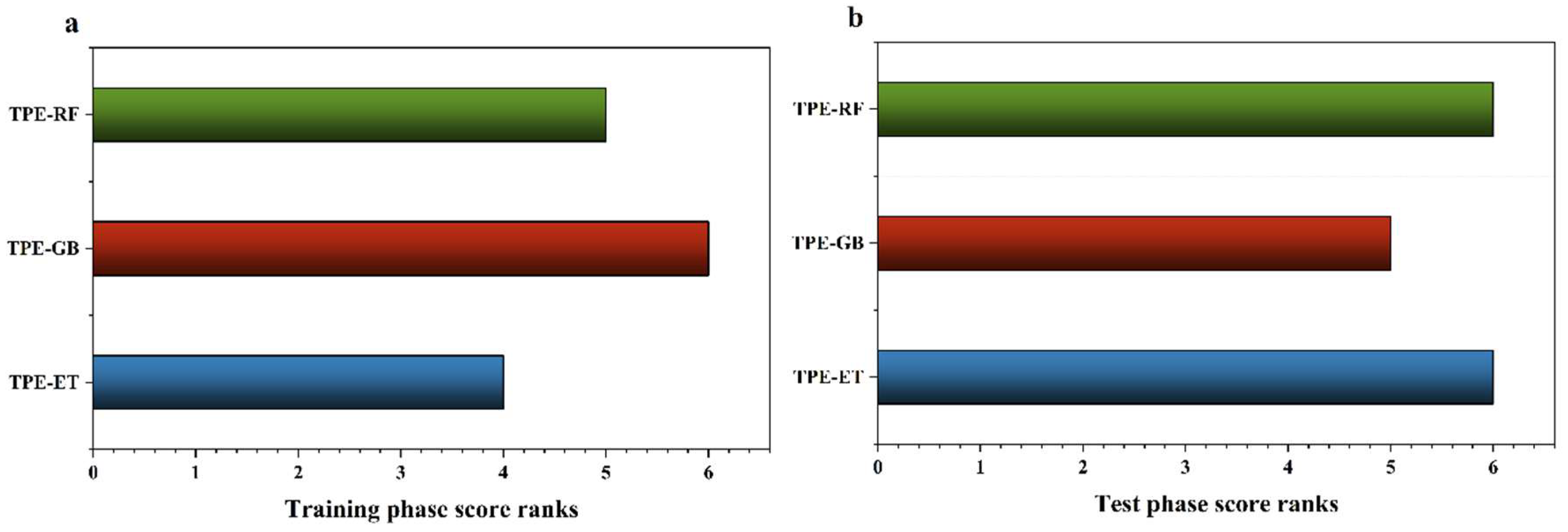
| Models | R2 | RMSE | MAE | Max Error | Scores |
|---|---|---|---|---|---|
| TPE-ET | 0.97 | 0.03 | 0.02 | 0.14 | |
| Rank | 1 | 1 | 1 | 1 | 4 |
| TPE-GB | 0.97 | 0.03 | 0.02 | 0.11 | |
| Rank | 1 | 1 | 1 | 3 | 6 |
| TPE-RF | 0.97 | 0.03 | 0.02 | 0.12 | |
| Rank | 1 | 1 | 1 | 2 | 5 |
| Models | R2 | RMSE | MAE | Max Error | Scores |
|---|---|---|---|---|---|
| TPE-ET | 0.93 | 0.04 | 0.03 | 0.25 | |
| Rank | 1 | 1 | 1 | 3 | 6 |
| TPE-GB | 0.92 | 0.04 | 0.03 | 0.28 | |
| Rank | 2 | 1 | 1 | 1 | 5 |
| TPE-RF | 0.92 | 0.04 | 0.03 | 0.26 | |
| Rank | 2 | 1 | 1 | 2 | 6 |
Disclaimer/Publisher’s Note: The statements, opinions and data contained in all publications are solely those of the individual author(s) and contributor(s) and not of MDPI and/or the editor(s). MDPI and/or the editor(s) disclaim responsibility for any injury to people or property resulting from any ideas, methods, instructions or products referred to in the content. |
© 2025 by the authors. Licensee MDPI, Basel, Switzerland. This article is an open access article distributed under the terms and conditions of the Creative Commons Attribution (CC BY) license (https://creativecommons.org/licenses/by/4.0/).
Share and Cite
Mame, M.; Huang, S.; Li, C.; Zhou, J. Application of Extra-Trees Regression and Tree-Structured Parzen Estimators Optimization Algorithm to Predict Blast-Induced Mean Fragmentation Size in Open-Pit Mines. Appl. Sci. 2025, 15, 8363. https://doi.org/10.3390/app15158363
Mame M, Huang S, Li C, Zhou J. Application of Extra-Trees Regression and Tree-Structured Parzen Estimators Optimization Algorithm to Predict Blast-Induced Mean Fragmentation Size in Open-Pit Mines. Applied Sciences. 2025; 15(15):8363. https://doi.org/10.3390/app15158363
Chicago/Turabian StyleMame, Madalitso, Shuai Huang, Chuanqi Li, and Jian Zhou. 2025. "Application of Extra-Trees Regression and Tree-Structured Parzen Estimators Optimization Algorithm to Predict Blast-Induced Mean Fragmentation Size in Open-Pit Mines" Applied Sciences 15, no. 15: 8363. https://doi.org/10.3390/app15158363
APA StyleMame, M., Huang, S., Li, C., & Zhou, J. (2025). Application of Extra-Trees Regression and Tree-Structured Parzen Estimators Optimization Algorithm to Predict Blast-Induced Mean Fragmentation Size in Open-Pit Mines. Applied Sciences, 15(15), 8363. https://doi.org/10.3390/app15158363