Real-Time Geo-Localization for Land Vehicles Using LIV-SLAM and Referenced Satellite Imagery

Featured Application

The proposed geo-localization method operates independently of satellite-based navigation systems and enables robust and drift-free global positioning over long-range navigation, making it particularly suitable for autonomous navigation of ground vehicles in GNSS-denied environments.

Abstract

Existing Simultaneous Localization and Mapping (SLAM) algorithms provide precise local pose estimation and real-time scene reconstruction, widely applied in autonomous navigation for land vehicles. However, the odometry of SLAM algorithms exhibits localization drift and error divergence over long-distance operations due to the lack of inherent global constraints. In this paper, we propose a real-time geo-localization method for land vehicles, which only relies on a LiDAR-inertial-visual SLAM (LIV-SLAM) and a referenced image. The proposed method enables long-distance navigation without requiring GPS or loop closure, while eliminating accumulated localization errors. To achieve this, the local map constructed by SLAM is real-timely projected onto a downward-view image, and a highly efficient cross modal matching algorithm is proposed to estimate the global position by aligning the projected local image to a geo-referenced satellite image. The cross-modal algorithm leverages dense texture orientation features, ensuring robustness against cross-modal distortion and local scene changes, and supports efficient correlation in the frequency domain for real-time performance. We also propose a novel adaptive Kalman filter (AKF) to integrate the global position provided by the cross-modal matching and the pose estimated by LIV-SLAM. The proposed AKF is designed to effectively handle observation delays and asynchronous updates while simultaneously rejecting the impact of erroneous matches through an Observation-Aware Gain Scaling (OAGS) mechanism. We verify the proposed algorithm through R³LIVE and NCLT datasets, demonstrating superior computational efficiency, reliability, and accuracy compared to existing methods.

1. Introduction

Autonomous navigation has drawn significant attention over the past years for its potential application in unmanned system. SLAM enables localization and mapping in GNSS-denied environments, making it a crucial and widely adopted technology for autonomous navigation across various applications [1,2]. Over the years, SLAM has undergone significant advancements, transitioning from pure vision-based approaches to more robust multi-sensor fusion methods that integrate LiDAR, inertial measurement units (IMU), and cameras to enhance localization accuracy and robustness. The most cutting-edge and advanced LIV-SLAM systems [3,4,5,6] exploit the depth accuracy of LiDAR, the motion constraints of IMU, and the feature richness of vision sensors to achieve high-precision and reliable localization and mapping in complex, real-world environments.

Despite the significant improvements achieved by the recent works, SLAM still faces several challenges. One major issue is the accumulation of errors over long-distance operation, leading to localization drift and map distortion. Additionally, global optimization for correcting accumulated errors in SLAM systems depends heavily on loop closure detection [7,8,9,10]. However, in many real-world scenarios, loop closures may be absent or challenging to detect.

Motivated by the limits of current methods and practical demands, we proposed a real-time geo-localizing navigation method for land vehicles that relies only on a LIV-SLAM and a referenced image. Our method is designed to function without GPS or loop closure. Instead, it estimates the global position by aligning the real-time constructed map to a referenced image with an efficient cross modal matching algorithm.

This paper makes three main contributions:

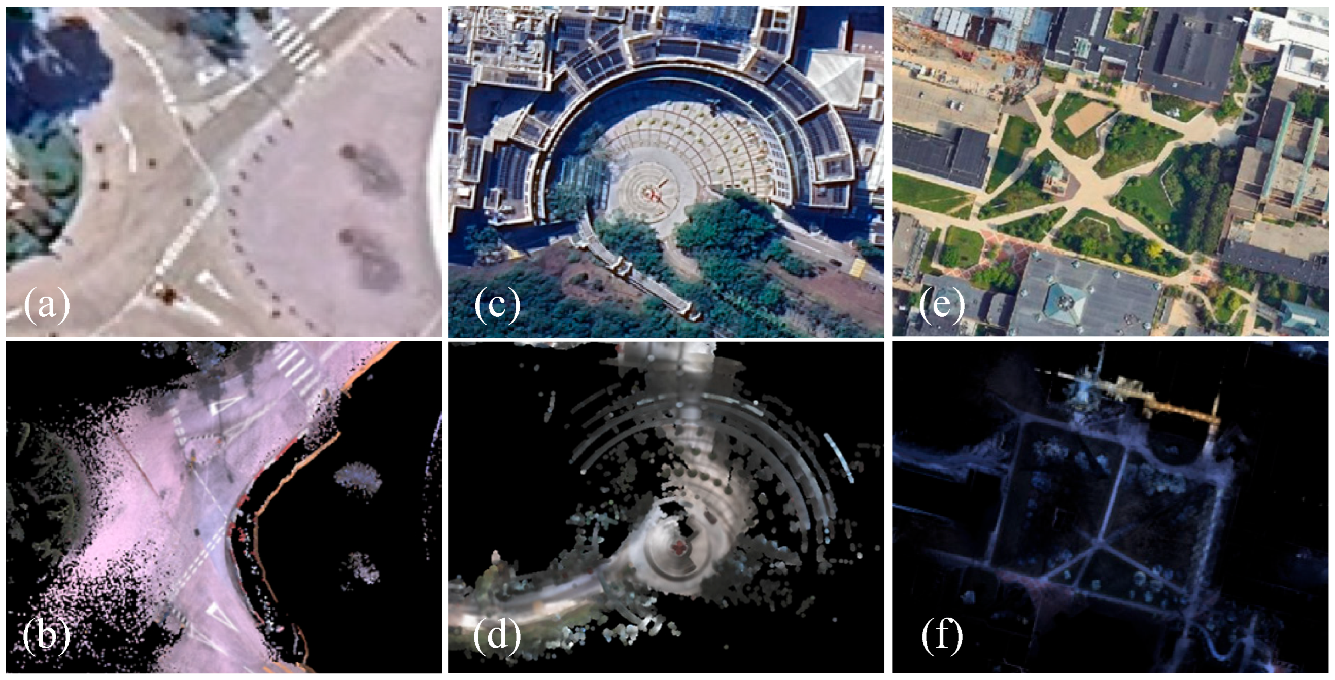
(1) A fast and robust cross-modal matching algorithm is proposed for the real-time geo-localization for land vehicles. The matching algorithm is designed to address the distortion caused by cross-modal, downward-view projection and cross-temporal scene variations, as shown in Figure 1. Figure 1a,b demonstrate cross-modal distortion, where the grayscale appearance of the same object varies significantly across modalities. Figure 1c,d depict projecting distortion, in which the object’s appearance changes due to geometric transformation. Figure 1e,f show scene variations resulting from temporal discrepancies between the projection image and the referenced image. Notably, all projection images contain invalid regions, typically visualized as black areas, which may introduce ambiguity and reduce the robustness of the matching process. We exploit Dense Structure Principal Direction (DSPD) [11] to capture gradient-orientation-based texture patterns, which remains consistent for cross-domain images.

Furthermore, the similarity measurement is optimized, and the searching efficiency is significantly improved with a fast correlation in the frequency domain. The comparison in the ablation experiments demonstrates that the proposed cross-modal matching algorithm achieved the best result in both accuracy and efficiency. A detailed comparative evaluation of different matching algorithms is presented in Section 4.3.1, which clearly shows the superior performance of our method in terms of matching precision and computational speed.

(2) This paper proposes an adaptive Kalman filter based on motion compensation (MC) and an Observation-Aware Gain Scaling (OAGS) mechanism. With motion compensation, the proposed AKF effectively eliminates prediction errors caused by observation delays and asynchronous updates. Ablation experiments demonstrate that MC effectively mitigates the adverse effects of observation delay, preventing degradation in fused localization accuracy, as detailed in the comparison of filters presented in Section 4.3.2. The OAGS mechanism dynamically adjusts the Kalman gain based on the matching coefficient, prediction deviation, and matching inconsistency, minimizing the adverse impact of incorrect matches on state estimation. This enhancement enables the proposed matching-based autonomous navigation approach to more effectively adapt to complex environmental variations, ensuring robust and reliable localization, as validated by the experimental results in Section 4.2 (Adaptability Evaluation) and Section 4.3.2 (Comparison of Filters).

(3) Building on the contributions above, we propose a novel and practical long-distance autonomous navigation approach for land vehicles. The proposed method is evaluated on the R³LIVE [3,4] and NCLT [12] datasets, demonstrating its effectiveness in diverse real-world scenarios. Experimental results show that the proposed method enables real-time global localization and effectively addresses the issue of position drift in LIV-SLAM systems. It achieves an average RMSE of 2.03 m across all sequences of the NCLT dataset in outdoor environments and 2.64 m on the R³LIVE dataset under the same condition.

To clarify the scope of this work, it should be noted that the goal of our research is not to present a universally optimal global localization solution. Rather, we aim to address a practical and increasingly common scenario: autonomous navigation in GNSS-denied environments where LiDAR and visual sensors are available.

2. Related Work

2.1. SLAM

SLAM has evolved significantly with the integration of multi-sensor fusion techniques.

Pure visual-based SLAM (VSLAM) systems, such as Mono-SLAM [13] and PTAM [14], rely solely on cameras to estimate motion and reconstruct the surrounding environment by extracting and tracking visual features across the frame, which suffers from limitations such as scale ambiguity in monocular setups and sensitivity to lighting variations and texture-less environments.

To address these issues, Visual-Inertial SLAM (VI-SLAM) integrates an IMU with visual data, leveraging the IMU’s short-term motion constraints to enhance motion estimation. Representative VIO-SLAM systems include OKVIS [15], VINS-Mono [16], and ORB-SLAM3 [9], which achieve improved robustness in dynamic or visually degraded conditions by tightly coupling visual and inertial data.

LIV-SLAM integrates LiDAR, IMU, and cameras, leveraging the strengths of each sensor to achieve high-precision localization and detailed scene reconstruction. State-of-the-art systems such as R³LIVE [3], R³LIVE++ [4], and Fast-LIVO [5,6] exploit tight LiDAR-visual-inertial fusion to enhance robustness in complex environments. By combining LiDAR’s depth accuracy, IMU’s motion constraints, and visual data’s rich feature representation, LIV-SLAM has become a leading solution for applications such as autonomous navigation, real-time mapping, and virtual reality.

Despite these advancements, challenges remain in real-time computation, large-scale map maintenance, and drift resistance, necessitating further research into efficient multi-sensor fusion strategies.

2.2. Matching Based Global Localization for Land Vehicles

Matching-based global localization typically matches a real-time image with a referenced image or referenced database, which determines geographic position without relying on GPS.

Street-view image matching (SVIM) is a commonly used visual geo-localization technique for land vehicles. It estimates the location of a query image by matching it to a geo-referenced street-view database [17,18,19,20,21,22,23,24]. Most existing SVIM algorithms adopt a retrieval approach, in which the distance between feature embeddings represents the likelihood that two images originate from the same or nearby locations. During inference, nearest neighbor search is performed within the database to find the best match for a given query image. However, this approach often results in limited localization accuracy because the referenced street-view image databases are not dense enough. Furthermore, the SVIM-based applications are often constrained by the incomplete coverage of street-view image databases [25].

Aerial and satellite images offer more extensive and higher-density coverage of outdoor areas than street-view databases, while also enabling efficient acquisition and frequent updates. Cross-view matching methods enable global localization by aligning ground-level images to aerial or satellite referenced images. Deep learning-based approaches, such as CVM-Net [26], utilize Siamese networks to learn viewpoint-invariant feature embeddings, while L2LTR [27] and TransGeo [28] further enhance the matching performance though attention model and positional encoding. Deuser et al. introduced Sample4Geo [29], a contrastive learning-based method leveraging symmetric InfoNCE loss [30,31], which incorporates hard negatives during training to enhance overall accuracy. More recently, Fervers et al. proposed a novel search region layout with consistent cell resolutions, enabling statewide visual geo-localization [25].

Hu and Lee [32] have explored the integration of cross-view matching into autonomous navigation systems using a probabilistic state estimation framework, which improves ground-to-aerial geo-localization through temporal consistency. This work has successfully realized long-distance, drift-free autonomous navigation for land vehicles, and the experiment results show that an average localization accuracy of approximately 20 m can be achieved.

However, cross-view matching methods are typically based on image retrieval techniques, which struggle with precise alignment between query images and reference maps, limiting the localization accuracy [25].

3. Materials and Methods

3.1. System Overview

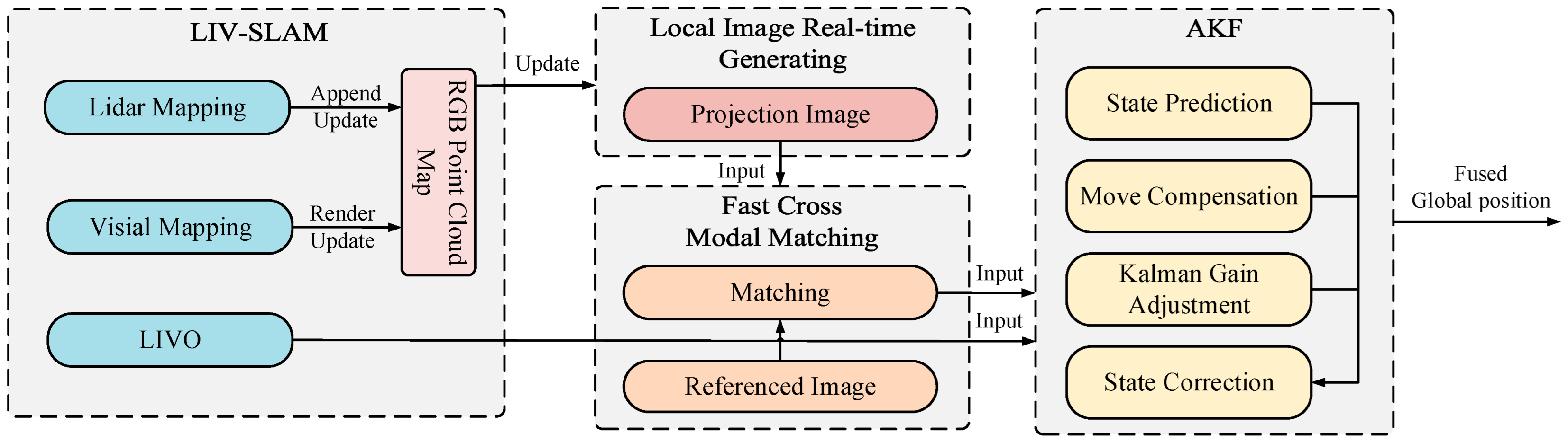
The overall framework of our system is illustrated in Figure 2, consisting of four main components: LIV-SLAM, local image real-time generating (Section 3.2), fast cross-modal image matching (Section 3.3), and AKF (Section 3.4).

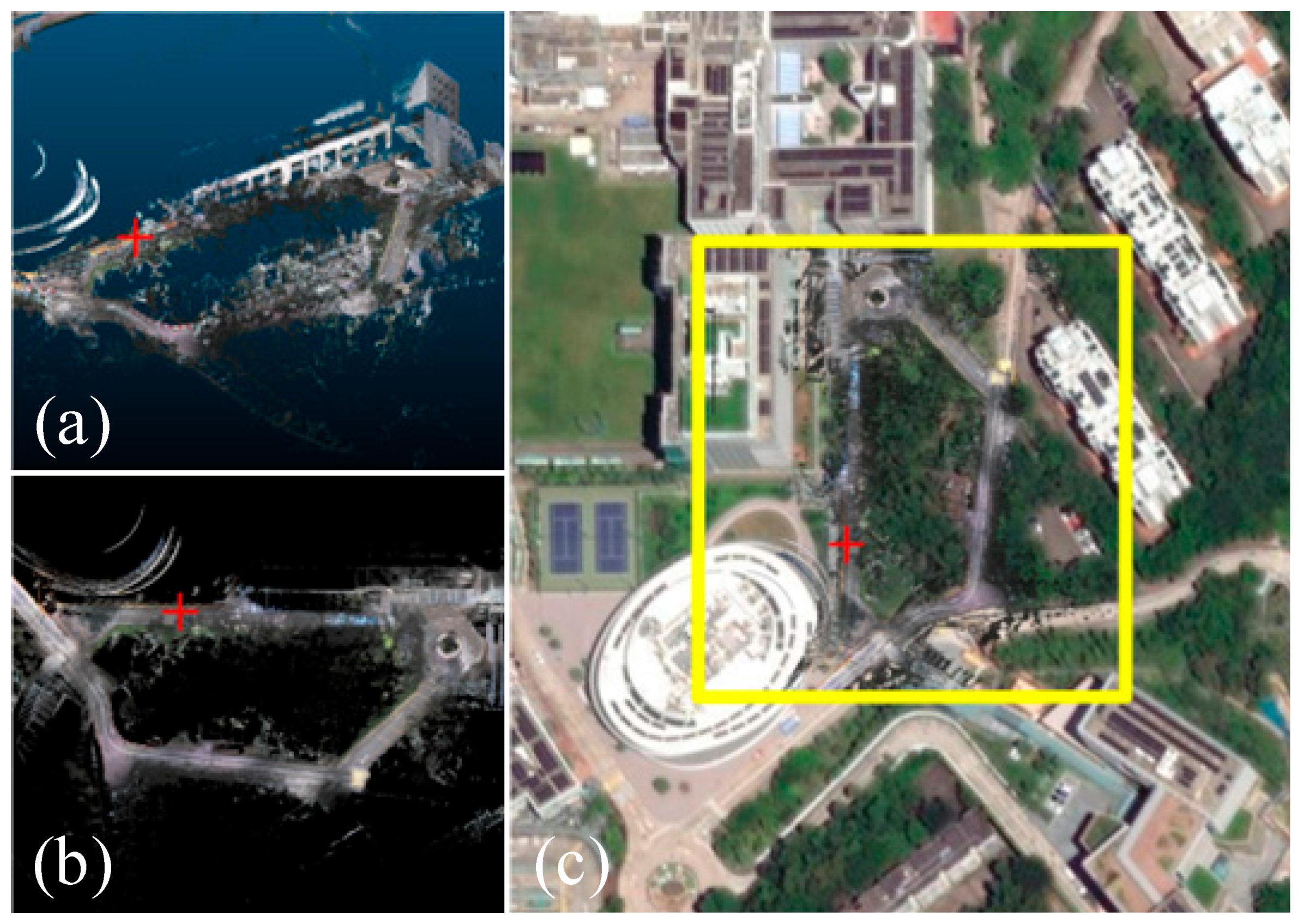
In our system, an existing LIV-SLAM framework is utilized for pose estimation and environment reconstruction. During the mapping process, the newly updated RGB point cloud, as shown in Figure 3a, is fed into a local image real-time generating algorithm. This method effectively addresses the cross-view challenge by incrementally projecting the local observations into a vertical downward-view image, as shown in Figure 3b. The fast cross-modal image matching module then aligns the projected image with the referenced image to get an absolute position in the referenced frame, as shown in Figure 3c. Finally, the AKF module fuses the horizontal speed estimated by LIV-SLAM with the global position obtained from the fast cross-modal image matching algorithm. This integration provides a refined position expressed in the coordinate frame of the referenced image.

Notably, the LIV-SLAM module can be implemented using various state-of-the-art methods, such as Fast-LIO [33,34], R³LIVE [3], R³LIVE++ [4], Fast-LIVO [6,7] and so on. Although Fast-LIO is primarily a LiDAR-inertial odometry, the RGB point cloud map can be rendered through the extrinsic parameters obtained by the calibration between LiDAR and camera. The referenced satellite imagery used in our method is preloaded and stored locally on the onboard computer. No online map services or downloads are required during runtime.

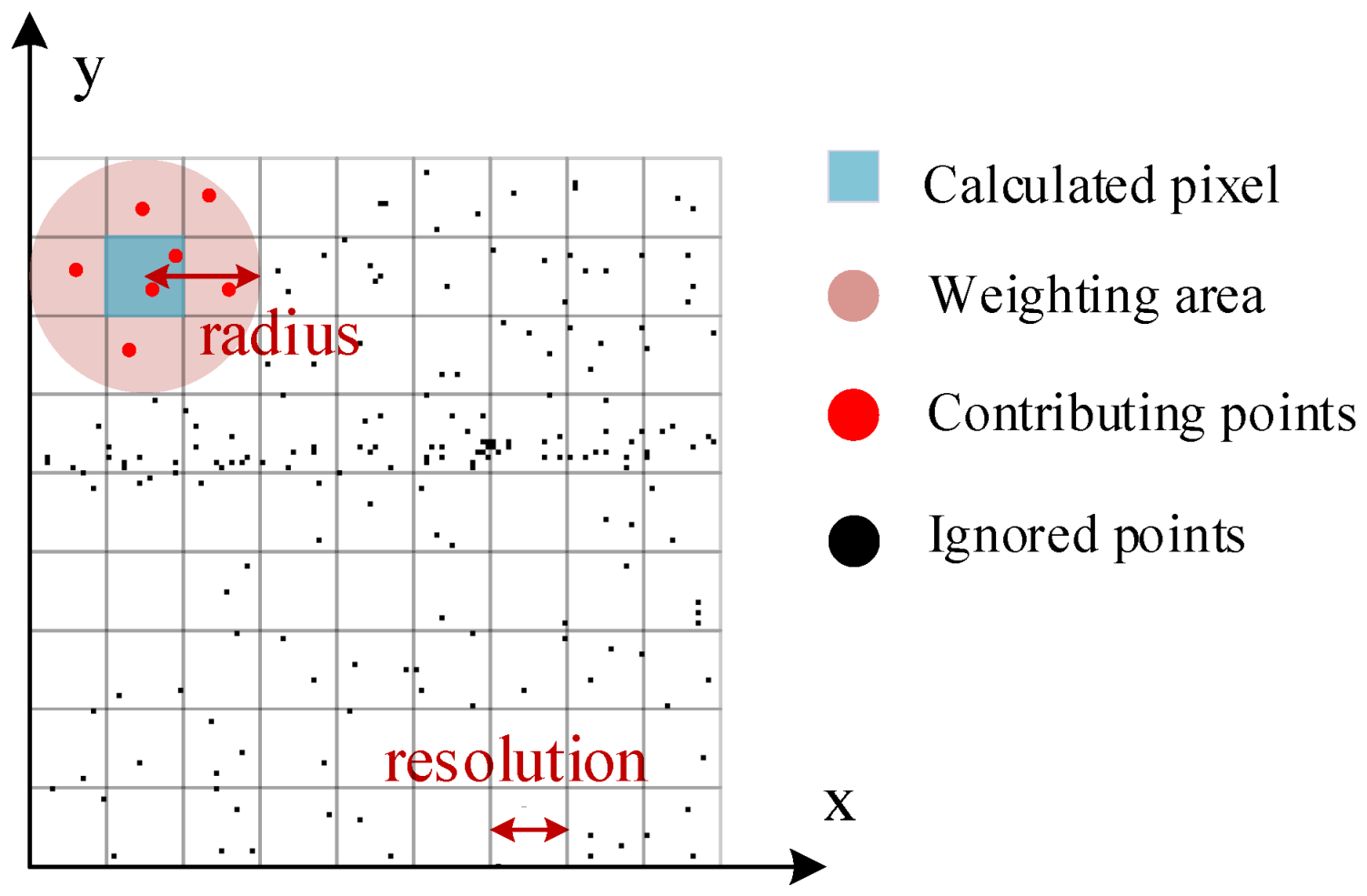
3.2. Local Image Real-Time Generating

The local image generating algorithm integrates features from multiple LiDAR scans and camera frames, thereby significantly enhancing the feature richness compared to single-view approaches.

Figure 4 gives the details of the projection.

Given a point set:

$$P=\left\{x,y,z,r,g,b\right\}$$

(1)

where $(x,y,z)$ represents the three-dimensional spatial coordinates, and $(r,g,b)$ represents the corresponding color information. For each pixel at $\left(c_x,c_y\right)$, a subset of $P$ within a radius is selected as contributing points, denoted as $D$. A projection map can be calculated using a Gaussian-weighted averaging method as follows:

$$I_i\left(c_x,c_y\right)={\displaystyle \frac{{\sum }_{p_k\in D}{p}_k\left(C_i\right)e^{-d_k^2/2{\sigma }^2}}{{\sum }_{p_k\in D}{e}^{-d_k^2/2{\sigma }^2}}}$$

(2)

where $d_k$ denotes the Euclidean distance between point $p_k$ and the calculated pixel $\left(c_x,c_y\right)$, $\sigma$ is the standard deviation, and $i$ represents the color channel, as each channel of the color $(r,g,b)$ is averaged in the same manner.

A straightforward implementation can be adopted. First, a projection image is determined based on the size of the projection area and the specified resolution. The color of each pixel is then computed using Equation (2), as illustrated in Figure 4. Assuming the image size is $n\times n$ and there are $m_1$ points within the projection area, the computational complexity of the approach is $O\left(n^2{m}_1\right)$. It is evident that this complexity increases rapidly with larger projection areas and finer resolutions.

To reduce computational overhead, the projection process is designed in an incremental way, using only the updated point cloud from the LIV-SLAM module. Specifically, each new point is projected onto the pixels within its effective weighting area. The numerator and denominator of (2) are accumulated into a value map $V\left(c_x,c_y\right)$ and a weight map $W\left(c_x,c_y\right)$, respectively. Then, the local projection image is generated by pixel-wise division of the value map by the weight map as follows:

$$I_i\left(c_x,c_y\right)={\displaystyle \frac{V\left(c_x,c_y\right)}{W\left(c_x,c_y\right)}}$$

(3)

The computational complexities of the first and second steps are $O\left(r^2{m}_2\right)$ and $O\left(n^2\right)$, respectively, where $r\times r$ is the size of the effective weighting area for a single pixel, and $m_2$ represents the number of updated points. Typically, the weighting region for a single pixel is much smaller than the entire projection area ($r \ll n$), and the number of updated points is significantly less than the total number of points within the projection area ($m_2\ll m_1$). As a result, the incremental implementation is considerably more efficient. Moreover, the computational complexity remains invariant by increases in image size or resolution, which enhances matching reliability and accuracy by allowing larger projection images to capture more distinctive and detailed features.

3.3. Fast Cross-Modal Matching

To address the distortions illustrated in Figure 1, we proposed a fast cross-modal matching algorithm based on DSPD [11]. DSPD is a feature descriptor based on structural orientation of images, which can effectively adapt to nonlinear intensity variations across different imaging modalities. Although the DSPD feature is robust to cross-modal distortions, it does not consider the invalid regions caused by the projection as shown in Figure 1. Besides, the matching algorithm proposed in [11] suffers from high computational cost, as its similarity metric requires full searching in spatial domain and the affine searching, which in this algorithm leads to excessive search redundancy for the matching between local projection image and the referenced image, which only has translational uncertainty.

To enhance the computational efficiency, we optimize the similarity metric and employ translation full searching, which can be realized with fast correlations in the frequency domain. Specifically, the dissimilarity metric proposed in [11] can be written to a similarity metric defined as follows:

$$S={\sum }_P\left|{\displaystyle \frac{\pi }{2}} - \left|{\alpha }_P - {\beta }_P\right|\right|, {\alpha }_P,{\beta }_P ϵ\left[-{\displaystyle \frac{\pi }{2}},{\displaystyle \frac{\pi }{2}}\right]$$

(4)

where ${\alpha }_P$ denotes the DSPD at a pixel of the projection image, and ${\beta }_P$ denotes the DSPD at the corresponding pixel of the referenced image.

To incorporate fast correlation in the frequency domain, we modify the similarity metric in (4) by introducing a double-angle cosine similarity as below:

$$S=\sum _P\mathit{cos}(2{\alpha }_P - 2{\beta }_P)$$

(5)

Both metrics give minimal similarity when the two DSPDs are mutually orthogonal and maximal similarity when they are parallel. Actually, Equation (5) can be derived from Equation (4) according to Fourier expansion. The detailed derivation of the equations is provided in the Supplementary Materials.

Furthermore, the translation full searching-based matching with the double-angle cosine similarity metric can be expressed in the form of two correlations, as shown in (6):

$$S=\sum _P{m}_p\mathit{cos}2{\alpha }_P\mathit{cos}2{\beta }_P+\sum _P{m}_p\mathit{sin}2{\alpha }_P\mathit{sin}2{\beta }_P$$

(6)

where $m_p$ is the mask of the projection image, which can be obtained during the projection process by binarizing the weight map. It is used to eliminate the influence of invalid regions in the projection image on the matching performance, as illustrated in Figure 1.

According to the convolution theorem, the full searching in the correlation of spatial domains can be efficiently implemented in frequency domain with Fast Fourier Transform (FFT) [35].

The translation full-searching with the similarity metric presented in Equation (4) has to be realized in the spatial domain. Given a projection image of size N × N and a search area of size M × M, the computational complexity of the full searching in the spatial domain is $O\left(N^2{(M - N+1)}^2\right)$. In contrast, the translation full-searching with the similarity metric presented in (6) can be realized in the frequency domain, where the FFT dominates the computational cost, resulting in an overall complexity of $O\left({2M}^{2}logM\right)$ [35]. The comparison of matching algorithms in ablation experiments (Section 4.3) demonstrates that the optimization significantly enhances the computational efficiency while maintaining the matching accuracy.

3.4. AKF Based on MC and OAGS

(1) Model: The system state $\mathit{x}$ of the proposed AKF is given as below:

$$\mathit{x}={\left[{\mathit{p}}^T,{\mathit{v}}^T,{\mathit{a}}^T\right]}^T$$

(7)

where the three sub-vectors ${\mathit{p}}^T,{\mathit{v}}^T,{\mathit{a}}^T$ denote the position, velocity, and acceleration in a horizontal direction, respectively. The process model of the proposed AKF is a typical motion model, which can be expressed as follows:

$${\stackrel{⌵}{\mathit{x}}}_t=F{\widehat{\mathit{x}}}_{t - 1}+N_a, N_a~\mathrm{N}\left(0,{\sigma }_a\right)$$

(8)

where ${\stackrel{⌵}{x}}_t$ and ${\widehat{x}}_t$represent the prior estimation and posterior estimate of the state at time $t$, $F$ gives the transition of the system state over time, and the process noise $N_a$ is attributed to uncertainties in acceleration.

The position observations are passed by the cross-modal matching algorithm, while the LIV-SLAM submodule provides the measurements of velocity, leading to the measurement model as follows:

$$\mathit{z}=H{\mathit{x}}_m+N_m$$

(9)

where $x_m$ contains the measurement of position and velocity, $H$ represents an identity matrix, and the measurement noise $N_m$ consists of position noise and velocity noise, defined as follows:

$$N_m~\left(\begin{array}{c}N(0,{\sigma }_{{\mathit{p}}_m})\\ N(0,{\sigma }_{{\mathit{v}}_m})\end{array}\right)$$

(10)

(2) Challenges: Since the observations are obtained from two independent submodules, there will be data latency and synchronization issues. Both the position and the velocity observations are subject to a certain delay due to the processing time before being input into the filter. Additionally, there is a discrepancy in update frequencies between position and velocity observations. Error position observation is another challenge. Although our cross-modal matching algorithm can adapt to image distortions to a certain extent, localization may degrade or even fail in the presence of significant scene changes or heavy occlusions or during transitions into indoor environments.

(3) Motion Compensation (MC): In the proposed method, historical observational data and the estimated navigation states output by the AKF are retained. The position observations are compensated using the past velocity observations, while the velocity observations are compensated based on historical acceleration estimations. This compensation mechanism enables the Kalman filter to process asynchronous data in a temporally consistent manner, ensuring fixed-frequency operation while minimizing the impact of observational delays, as shown in Figure 5. The effectiveness of MC is validated in the comparison of filters in ablation experiments (Section 4.3).

(4) Observation-Aware Gain Scaling (OAGS): To evaluate the confidence of position observations, we leverage the three indicators as follows:

• Matching coefficient: This refers to the value of the similarity metric defined in (6), which is an indicator of matching reliability. A higher matching coefficient means a higher confidence level for a position observation, and vice versa.
• Matching inconsistency: After the initial matching, the sub-patches of the projection image will be re-searched in corresponding sub-searching areas. The matching inconsistency $T$ is calculated as follows:

  $$T={\sum }_i‖t_i-t‖$$

  (11)

  where $t$ is the translation estimated with the projection image, and $t_i$ is the translation estimated with a sub-patch. A large matching inconsistency typically suggests that the associated position observation is incorrect.

• Prediction deviation: We evaluate the deviation between the predicted state of the Kalman filter and the position observation obtained from the cross-modal matching. A large deviation is highly indicative of the position observation being erroneous.

The three indicators are normalized and utilized as input to the sigmoid function, which is defined as follows:

$$h\left(\mathit{y}\right)={\displaystyle \frac{1}{1+e^{-\alpha \left({\mathit{\theta }}^T\mathit{y}\right)+\beta }}}$$

(12)

This function gives the relationship between the confidence of position $h\left(\mathit{y}\right)$ and the three indicators (denoted as vector $\mathit{y}$). $\mathit{\theta }$ is a weighted vector, and $\alpha$ and $\beta$ are linear transformation parameters. Based on the observation that the matching coefficient is positively correlated with the confidence of the matching result, while the latter two indicators are negatively correlated with it, the parameter $\mathit{\theta }$ is set as $\left[1,-1,-1\right]$, the scaling factor is set to 10 to effectively amplify the effect of $\mathit{\theta }$, and the bias term $\beta$ is set to 0. This configuration is fixed through all our experiments.

Based on the evaluation of position observation confidence, the OAGS is formulated as below:

$$\widehat{K}=h\left(\mathit{y}\right)K$$

(13)

$${\widehat{\mathit{p}}}_t={\stackrel{⌵}{\mathit{p}}}_t+\widehat{K}\left(\mathit{Z}-H{\mathit{p}}_m\right)$$

(14)

$${\widehat{E}}_t=\left(I-\widehat{K}H\right){\stackrel{⌵}{E}}_t$$

(15)

where $K$ represents the original Kalman gain, the position-related components of which are adaptively adjusted based on the confidence of the position observation, denoted as $h\left(\mathit{y}\right)$. Consequently, the updates to the position state ${\widehat{\mathit{p}}}_t$ and the covariance matrix ${\widehat{E}}_t$ are modified accordingly, as shown in Equations (14) and (15).

Equations (13) and (14) show that the filter places greater reliance on the observation when the confidence is high, while reducing the influence of the erroneous position observation when the confidence is low.

4. Experiments

To evaluate the performance of the proposed method, we conduct extensive experiments in public datasets, including the NCLT dataset [12] and R³LIVE dataset [3,4]. Both datasets contain LiDAR, IMU, and camera data. To better evaluate the position drift correction of the proposed method, we selected 14 long-distance sequences covering diverse environmental conditions.

Table 1. Comparison of APE (m) on NCLT dataset.

Sequence (Date)	Length (km)	Duration (s)	Ours (Outdoor)	R3LIVE++	Fast-LIO2
2012-02-02 1	6.2	5854.54	1.36	5.33	9.12
2012-02-04	5.5	4659.86	1.85	5.58	7.19
2012-02-05	6.5	5620.74	1.73	8.52	7.80
2012-02-19	6.2	5319.48	1.79	8.52	5.98
2012-03-17	5.8	4948.81	2.53	4.83	4.70
2012-03-25	5.8	4840.98	4.63	\ 2	19.30
2012-04-29	3.1	2597.90	1.28	6.32	6.44
2012-05-11	6.0	5073.34	2.54	3.70	4.13
2012-06-15	4.1	3310.51	1.78	7.74	5.27
2012-08-04	5.5	4814.31	1.91	3.85	6.96
2012-10-28	5.6	5138.99	1.33	7.71	7.68
2012-11-17	5.7	5315.78	1.68	8.68	5.83

¹ The dates represent the data acquisition dates of specific sequences from NCLT dataset. ² The original R³LIVE++ paper does not report experimental results on the 2012-03-25 sequence.

and

Table 2. Comparison of APE (m) on R³LIVE dataset.

Sequence	Length (km)	Duration (s)	Ours (Outdoor)	R3LIVE-	Fast-LIVO2
hkust-seq00	1.3	1073	1.92	4.68	4.88
hkust-seq01	1.5	1162	3.35	6.06	4.37

give the details of the selected sequences.

Localization accuracy is evaluated using the Absolute Position Error (APE), which is calculated in terms of RMSE:

$$\mathrm{R}\mathrm{M}\mathrm{S}\mathrm{E}=\sqrt{{\displaystyle \frac{1}{n}}\sum _{i=1}^n{‖{\widehat{\mathit{p}}}_i-{\mathit{p}}_i‖}^2}$$

(16)

where ${\widehat{p}}_i$ denotes the estimated position of the proposed method and $p_i$ is the corresponding position of ground truth.

Since matching-based positioning is infeasible indoors, some accuracy evaluations exclude all indoor results. Columns labeled as “outdoor” report statistics for outdoor localization only, while others include all results.

In our implementation, the projection area is set to 150 m × 150 m with an image resolution of 0.1 m/pixel, and the matching search radius is 20 m. The R³LIVE dataset was collected in August 2021, and the corresponding referenced imagery was collected in April 2022. The NCLT dataset used in our experiments was recorded in 2012 from February to November, and the corresponding referenced imagery was captured in April 2015. All referenced imagery was acquired from Google Earth at zoom level 19, with an approximate ground resolution of 0.2986 m/pixel. During processing, the referenced imagery was resampled to 0.1 m/pixel to maintain consistency with the resolution of the projection map.

4.1. Outdoor Accuracy Evaluation

To evaluate the localization accuracy of our proposed system, we conducted experiments on the NCLT dataset and compared the results with two representative SLAM algorithms: R³LIVE++ [4] and FAST-LIO2 [34]. None of the compared methods employed loop closure. Our method utilizes FAST-LIO2 as the odometry backbone.

The experimental results are shown in Table 1, demonstrating that the proposed method significantly improves localization accuracy compared to R³LIVE++ and FAST-LIO2. This improvement is primarily attributed to the use of global localization based on image matching, which effectively eliminates error accumulation over time.

It is worth noting that the original R³LIVE++ paper does not report experimental results on the 2012-03-25 sequence. Our experiments further indicate that Fast-LIO2 exhibits significant drift on this sequence, with an RMSE of 19.30 m. However, our proposed method effectively corrects the drift by integrating matching-based observations.

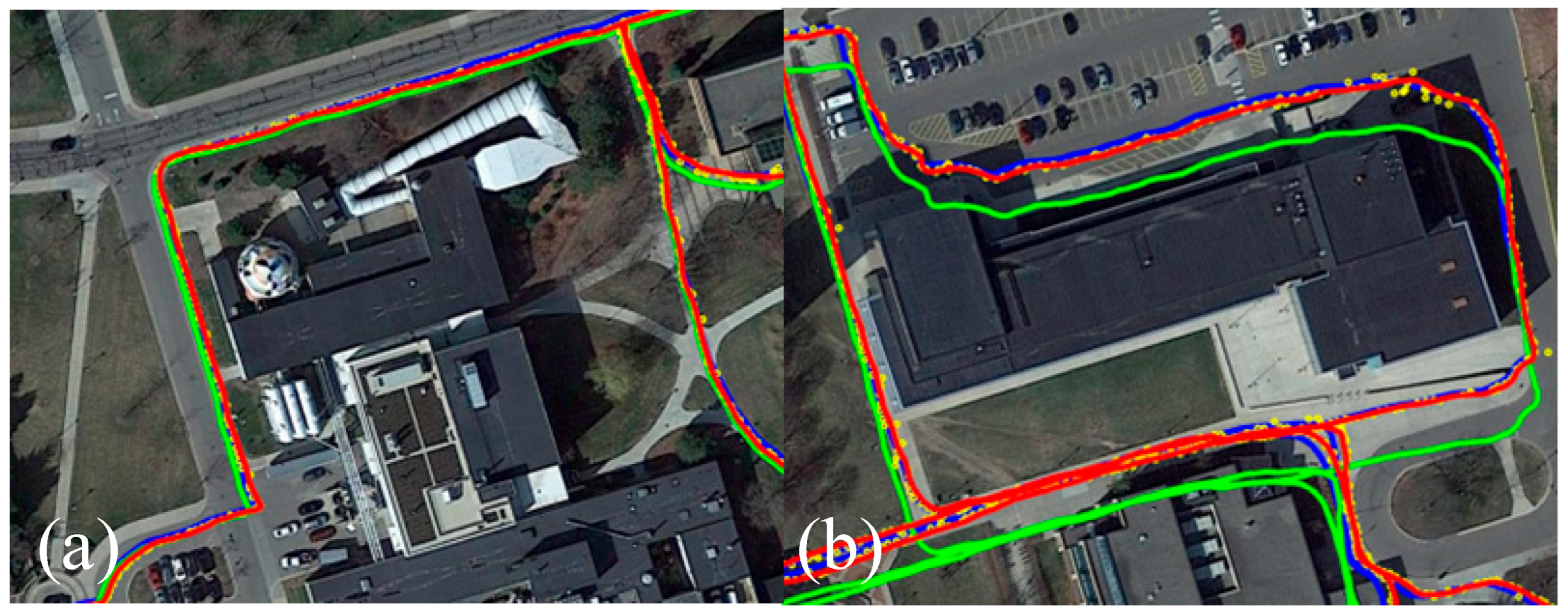
Figure 6 presents a comparison between the proposed method and FAST-LIO2 on a representative segment from the NCLT dataset. As shown in Figure 6, the green, red, and blue lines represent the trajectories estimated by LIV-SLAM (FAST-LIO2), the proposed method, and the ground truth, respectively, while the yellow points indicate the localization results obtained from the matching algorithm. This color convention is consistently used throughout the paper. In Figure 6a, the initial segment of a sequence from the NCLT dataset shows that FAST-LIO2 maintains low drift and achieves localization accuracy comparable to our method. However, in Figure 6b, after approximately 1800 s, FAST-LIO2 begins to exhibit significant position drift due to accumulated odometry error. In contrast, our method continuously corrects this drift through matching-based global localization, thereby achieving improved overall localization accuracy.

We also conducted comparative experiments on two sequences from the R³LIVE dataset, evaluating the proposed method against R³LIVE and Fast-LIVO2. Since the original R³LIVE, under default parameters, has been reported to achieve a localization accuracy of approximately 0.1 m [3], we use its trajectory as the ground truth reference for evaluation.

Table 2 shows the localization accuracy of the three methods on the R³LIVE dataset, also demonstrating that the proposed approach achieves the minimum RMSE among all tested methods. In Table 2, R³LIVE- is a degraded version of R³LIVE, which operates with reduced point cloud resolution and a smaller number of tracked visual features, resulting in degraded odometry performance. When comparing with the outputs of R³LIVE-, the LIV-SLAM module implemented in our system is also R³LIVE-. Therefore, the observed improvements in localization accuracy are solely attributed to the proposed method.

4.2. Adaptability Evaluation

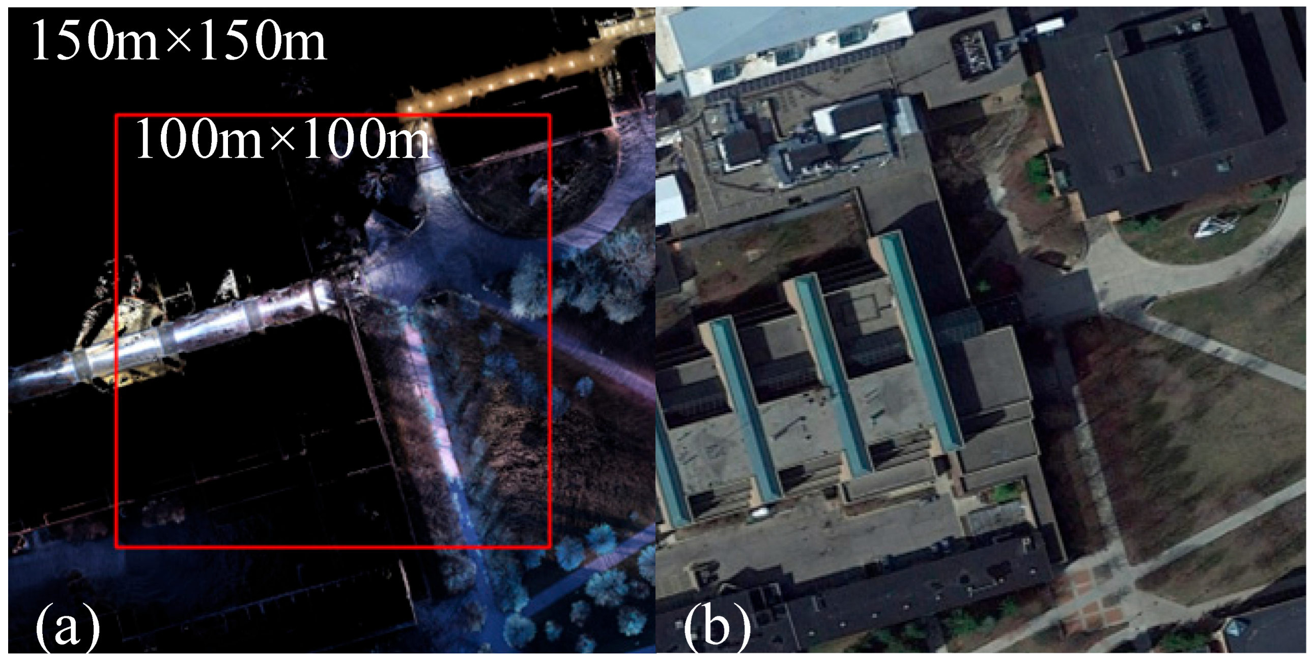
Significant scene variations and transitions into indoor environments may cause substantial discrepancies between real-time projection images and referenced images, thereby greatly reducing the reliability of image matching. To address this issue, two strategies can be adopted. First, enlarging the projection image area can help include more corresponding features, thus improving matching robustness. Figure 7 presents an example of indoor environment, where the red cross represents the current localization, Figure 7a,b show the projection image of the local region and its corresponding reference map, respectively. Compared to the 100 m × 100 m projection image, the 150 m × 150 m projection image includes a larger portion of the surrounding outdoor area, thereby capturing more features that effectively correspond to the reference image. Additionally, increasing the search range allows the matching algorithm to relocate the correct position after passing through disturbed or occluded regions.

Although the correct position can be relocated by increasing the search range, the fused localization accuracy will be still degraded due to the incorrect matching results. To mitigate this, the proposed OAGS mechanism adaptively adjusts the Kalman gain based on the matching confidence, thereby significantly suppressing the adverse impact of incorrect observations. As illustrated in Figure 8a, erroneous observations from image matching could lead to significant localization errors, while Figure 8b shows the result after applying the proposed OAGS mechanism. By effectively suppressing unreliable observations during indoor environments, the fusion trajectory with OAGS remains significantly closer to the ground truth, indicating a clear improvement in both localization robustness and accuracy.

4.3. Ablation Experiments

In this section, we conduct ablation experiments to evaluate the performance of the individual modules within the proposed framework.

4.3.1. Comparison of Matching Algorithm

The proposed matching algorithm is compared against other matching methods, including Scale Invariant Feature Transform (SIFT), omniGLUE [36], MI [37], and CFOG [38]. Among them, SIFT is a classic local feature-based algorithm, while omniGLUE is a more recent and deep learning-based feature matching method that can be applied to cross-modal matching tasks. Both MI and CFOG are designed for cross-modal matching. Similar to our method, they adopt a translation-based full-search strategy for the matching. Two variants of our method are included in the comparison: ASD, a spatial-domain search based on the absolute difference metric (4), and CFD, a frequency-domain search utilizing the double-angle cosine similarity metric (6).

A total of 100 matching pairs, each consisting of a real-time projection image and the corresponding reference search region, were randomly sampled from 14 sequences. A matching result is considered incorrect if its distance to the ground truth exceeds 5 m. The results in

Table 3. Comparison of matching performance.

Method	Accuracy	Processing Time (s)
SIFT	0%	1.67
OMNIGLUE	1%	126.59
MI	76%	265.32
CFOG	80%	0.31
Ours (ASD)	96%	5.50
Ours (CFD)	96%	0.02

demonstrate that our method achieves the best performance in terms of both matching accuracy rate and computational efficiency. Examples of the above matching method are provided in Figure 9.

4.3.2. Comparison of Filters

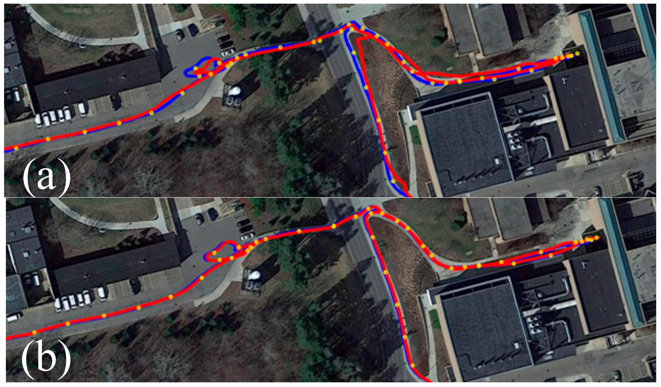
In this section, we compare the performance of three variants of the Kalman filter: the standard Kalman filter (KF), the Kalman filter with motion compensation (KF + MC), and the Kalman filter with both motion compensation and the proposed Observation-Aware Gain Scaling (KF + MC + OAGS). The standard KF and KF + MC were each evaluated under three different positioning update frequencies to assess the impact of observation delay on localization performance.

The evaluation results are summarized in

Table 4. Comparison of localization accuracy (APE, m) with and without MC.

Sequence	KF (Outdoor)			KF+MC (Outdoor)
	0.2 s	1 s	10 s	0.2 s	1 s	10 s
2012-02-02	1.40	1.32	5.61	1.34	1.36	1.30
2012-02-04	1.71	1.71	6.07	1.86	1.85	1.58
2012-02-05	1.73	1.69	6.07	1.73	1.73	1.85
2012-02-19	1.94	1.79	7.12	1.83	1.79	1.99
2012-03-17	2.66	2.51	6.72	2.44	2.53	2.85
2012-03-25	4.72	4.58	9.36	4.52	4.63	5.01
2012-04-29	1.19	1.15	5.54	1.21	1.28	1.09
2012-05-11	2.59	2.52	7.29	2.55	2.54	2.83
2012-06-15	1.73	1.56	6.27	1.65	1.78	2.04
2012-08-04	1.96	1.81	5.98	1.87	1.91	1.87
2012-10-28	1.61	1.33	21.39	1.35	1.33	1.34
2012-11-17	1.66	1.57	6.44	1.54	1.68	1.88
hkust-seq00	1.70	1.79	5.54	1.89	1.92	2.02
hkust-seq01	3.47	3.40	7.14	3.42	3.35	3.46

. The results show that as the localization observation frequency decreases (corresponding to increased observation delay from 1 s to 10 s), the standard KF suffers from significant degradation in localization accuracy. In contrast, KF with MC maintains better performance due to the integration of motion compensation. Figure 10 illustrates the trajectory segments of KF and KF + MC, highlighting the performance difference under a 10-s observation delay. Specifically, (a) shows the result of the standard KF, while (b) presents the corresponding trajectory obtained using KF + MC. The improvement is particularly evident in turning scenarios, where motion compensation effectively mitigates the impact of delayed observations.

Table 5. Comparison of localization accuracy (APE, m) with and without OAGS.

Sequence	OAGS Disabled	OAGS Enabled
2012-02-02	2.27	1.63
2012-02-04	2.20	1.47
2012-02-05	2.18	1.73
2012-02-19	2.17	1.83
2012-03-17	4.14	2.77
2012-03-25	4.90	5.89
2012-04-29	1.75	1.07
2012-05-11	2.74	2.72
2012-06-15	1.99	1.84
2012-08-04	1.94	1.71
2012-10-28	1.46	1.32
2012-11-17	1.68	1.66
hkust-seq00	2.34	2.28
hkust-seq01	12.65	8.55

presents the comparison between KF + MC and KF + MC + OAGS. The results show that enabling OAGS further reduces the overall RMSE. This improvement is primarily due to the ability of OAGS to suppress the influence of incorrect matching results, which can otherwise degrade the fused localization accuracy, particularly in indoor environments where the referenced image is unavailable.

4.4. Computational Efficiency

In this section, we evaluate the average processing time of the proposed method. The experiments were conducted on a PC equipped with an Intel i7-1360P CPU and 64 GB of RAM, without any GPU acceleration.

The main computational cost of the proposed algorithm lies in the projection and matching modules. Enabling the OAGS mechanism introduces additional overhead due to the evaluation of matching inconsistency.

Table 6. Processing time statistics.

Module	Projection	Matching	OAGS	Total
Average time (ms)	1.64	24.81	46.91	73.36

reports the average processing time of each submodule in single-threaded implementation. On the testing platform, the system runs at approximately 14 Hz with OAGS enabled and around 30 Hz without it.

5. Conclusions

This paper presents a global localization algorithm based on real-time map projection and cross-modal image matching, which can effectively correct the drift in existing LIV-SLAM systems such as Fast-LIO, R³LIVE++, and Fast-LIVO2. In addition, we propose an AKF incorporating MC and OAGS mechanisms, which fuses the outputs of the LIV-SLAM module with global localization results to achieve a novel and practical long-distance autonomous navigation approach for land vehicles.

Compared to existing cross view-based autonomous navigation approaches [32], which achieves an average localization accuracy of about 20 m and operates at a relatively low frequency of 0.5–1 Hz, the proposed method achieves pixel-level alignment, resulting in significantly improved localization accuracy (RMSE of about 2 m) and real-time performance (approximately 14 Hz with OAGS enabled and around 30 Hz without it).

However, the proposed method has several limitations. First, it requires accumulating a sufficient amount of point cloud data before generating a projection image, thus it cannot support one-shot localization. Second, the system relies on the output of a LIV-SLAM module; if the SLAM fails completely (e.g., due to extreme motion or sensor degradation), the localization may fail. Additionally, in environments lacking structural or texture features, such as open grasslands or deserts, the image matching process may be unreliable.

Future work will focus on extending the proposed framework to a purely vision-based solution that eliminates the dependency on LiDAR sensors. This adaptation will improve the system’s applicability to a broader range of platforms.

The Supplementary Materials which provide trajectory plots of the proposed method on all test sequences and a demo video will be released through GitHub (https://github.com/yao-yating/RGL-LIV-SLAM, accessed on 7 June 2025) and BaiduDisk (https://pan.baidu.com/s/1qoij3u7oM1qBKZjLjzg42Q?pwd=sa6q, accessed on 7 June 2025).