Local Back-Propagation for Forward-Forward Networks: Independent Unsupervised Layer-Wise Training

Abstract

Recent deep learning models, including GPT-4, have achieved remarkable performance using the back-propagation (BP) algorithm. However, the mechanism of BP is fundamentally different from how the human brain processes learning. To address this discrepancy, the Forward-Forward (FF) algorithm was introduced. Although FF enables deep learning without backward passes, it suffers from instability, dependence on artificial input construction, and limited generalizability. To overcome these challenges, we propose Local Back-Propagation (LBP), a method that integrates layer-wise unsupervised learning with standard inputs and conventional loss functions. Specifically, LBP demonstrates high training stability and competitive accuracy, significantly outperforming FF-based training methods. Moreover, LBP reduces memory usage by up to 48% compared to convolutional neural networks trained with back-propagation, making it particularly suitable for resource-constrained environments such as federated learning. These results suggest that LBP is a promising biologically inspired training method for decentralized deep learning.

1. Introduction

Recently, large language models have demonstrated performance that even surpasses human capabilities [1]. Much of this success is due to the back-propagation algorithm (BP) [2,3], supported by advancements in hardware technology. However, one criticism of BP is that it does not closely resemble the biological processes underlying brain function [4,5,6,7]. Another drawback is that BP, by relying on backward passes, requires all layers of a model to remain continuously connected during training. These limitations have motivated researchers to explore alternative learning mechanisms that are more biologically grounded and resource-efficient [8,9,10].

Among such efforts, the Forward-Forward (FF) algorithm [10] represents a recent and influential attempt to train deep networks using only forward passes. FF avoids backward gradient propagation by comparing two forward activations (positive and negative) using a local loss. This design opens new possibilities for local, interpretable, and distributed learning. However, FF presents notable drawbacks: it requires specially constructed input variants (positive, negative and neutral), a non-standard loss function, and exhibits instability across datasets. These issues significantly limit its applicability in conventional machine learning workflows and hinder its scalability. Furthermore, its performance has been shown to vary significantly across datasets and models, and its learning stability is limited.

To address some of these limitations, subsequent studies have proposed several enhancements. For example, the Self-Contrastive FF [11] improves sample construction and stability by refining the positive/negative sample definitions. The Integrated FF [12] incorporates shallow gradient signals to stabilize training. The On-Tiny-Device FF [13] demonstrates FF’s potential in constrained hardware settings by searching for FF-compatible initializations. However, these works still rely on the FF paradigm’s core assumption of specialized inputs and retain its inherent training instability. Furthermore, they do not explore the broader class of unsupervised learning models that may better support local layer-wise learning.

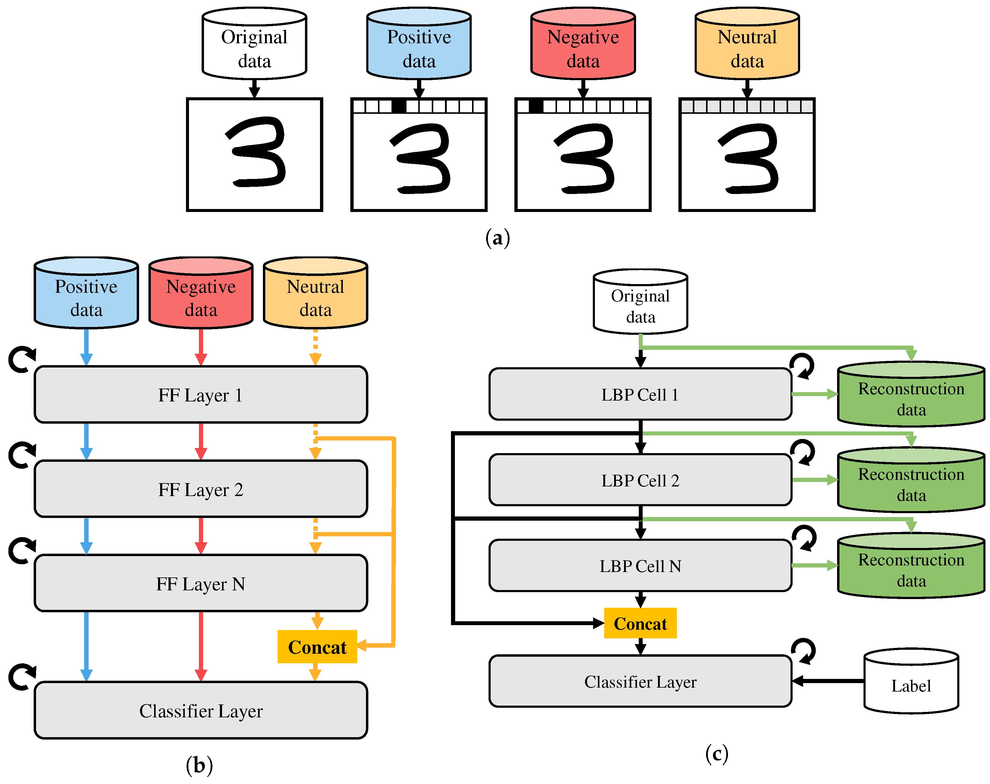
As shown in Figure 1, to overcome these gaps, we propose the Local Back-Propagation (LBP) algorithm, a forward-only training approach that replaces FF’s layer with a compact unsupervised model such as an Auto-Encoder (AE), Denoising AE (DAE), Convolutional AE (CAE), or Generative Adversarial Network (GAN). Unlike FF, our method works with standard inputs and common reconstruction or classification losses, removing the dependency on handcrafted positive and negative examples. Each LBP layer, referred to as a ‘cell’ in this paper, is trained independently to reconstruct its input, and its latent output is passed forward to the next cell. This layer-wise unsupervised learning retains the local update advantage of FF while improving stability, expressivity, and compatibility with practical data pipelines.

LBP is particularly well suited for federated and edge learning scenarios. Since each layer is trained independently, the entire model does not need to be loaded into memory during training. Layers can be trained sequentially using minimal memory, enabling the training of deep models on resource-constrained devices without requiring backward gradient computation or global synchronization.

We evaluate the LBP framework across various unsupervised cell types and datasets (MNIST, CIFAR-10, and CIFAR-100), and we further assess its effectiveness in federated learning setups. Our results show that LBP offers improved training stability and performance over FF, maintains compatibility with standard inputs and losses, and achieves performance levels that are competitive with simple CNNs, particularly in constrained settings.

Our main contributions are as follows:

• We propose Local Back-Propagation (LBP), a forward-only training algorithm that combines the structural efficiency of FF with the flexibility of unsupervised learning models.
• We demonstrate that LBP eliminates the need for specialized input construction and enables training with standard data and losses.
• We empirically validate LBP across several datasets and architectures, including federated learning scenarios where memory and communication are limited.

The remainder of this paper is organized as follows. Section 2 reviews related work. Section 3 presents the LBP algorithm and training procedure. Section 4 describes the experimental setup and results. Section 5 discusses the results in depth. We conclude this study in Section 6.

2. Related Works

2.1. Alternatives to Back-Propagation

Criticisms of BP from a biological standpoint primarily center on its backward pass, which does not align well with biological neural processes. In biological neural networks, neuron stimulus transmission is largely unidirectional, making a full backward pass difficult. Although reciprocal connections [14,15] do allow some form of backward flow, they are limited to local connections between adjacent neurons. This contrasts with the global feedback pathways required by BP. Furthermore, the weights in forward synapses do not symmetrically correspond to those in backward synapses, complicating feedback processes. To address these issues, alternative approaches such as Feedback Alignment [9] and Predictive Coding [8] have been proposed.

Feedback Alignment employs random weights for feedback during the weight update phase. This method has shown that learning can occur even when forward and backward weights are not strictly symmetrical. While BP involves complex calculations to synchronize forward and backward weights, Feedback Alignment suggests that similar performance can be achieved by maintaining consistent update directions through random values. Over multiple iterations, the learning process aligns these directions, indicating that BP’s requirements for strict weight symmetry may be unnecessarily rigid, and that Feedback Alignment can alleviate some biological criticisms of BP.

Predictive Coding, on the other hand, implements local feedback by having each layer predict the input of the subsequent layer. The loss is calculated by comparing the predicted input with the actual input, allowing weight updates between adjacent layers. Previous studies Whittington and Bogacz [16], Millidge et al. [17] have shown that Predictive Coding achieves performance comparable to BP in various models, including Multi-Layer Perceptrons (MLPs) [18], Convolutional Neural Networks (CNNs) [19], and Recurrent Neural Networks (RNNs) [20].

2.2. Applications and Limitations of the Forward-Forward Algorithm

The FF algorithm proposed by Hinton [10] introduced a training mechanism that replaces the backward pass with two forward passes using positive and negative samples. While FF is notable for its conceptual novelty and biological plausibility, it relies on handcrafted input variants and a non-standard loss function. These constraints limit its practicality in general-purpose learning tasks.

Several recent studies have attempted to improve upon FF’s limitations. Ororbia and Mali [21] integrate Predictive Coding with FF to ensure effective local layer-to-layer learning. Since the FF algorithm operates using only forward passes, closely resembling the function of the brain, it still requires verification of inter-layer information exchange. By incorporating Predictive Coding, Ororbia and Mali [21] have demonstrated that FF can achieve performance close to that of MLP models trained with BP.

The Self-Contrastive Forward-Forward algorithm [11] refines the construction of positive and negative samples by introducing a more stable contrastive formulation. The Integrated Forward-Forward method [12] introduces shallow gradient feedback to stabilize the learning process while retaining the forward-only property. Additionally, the On-Tiny-Device FF approach [13] investigates the viability of FF training on highly constrained devices by searching for initialization strategies that enhance convergence and performance.

An attempt to combine FF with federated learning [22] was made by FedFwd [23], aiming to validate its practicality in decentralized environments. While the approach showed promise, its performance remained lower than that of MLP models trained with BP.

These works share a common goal of improving the stability and applicability of FF, yet they still depend on the core FF structure and do not generalize to broader unsupervised models or standard data formats.

2.3. Layer-Wise Unsupervised Learning Approaches

In addition to these biologically motivated approaches, several studies have explored layer-wise unsupervised learning techniques since the early development of deep learning. Bengio et al. [24] proposed a greedy layer-wise training method using stacked AE, where each layer is trained to reconstruct its input before proceeding to the next. Vincent et al. [25] extended this idea by introducing DAE, which improved robustness through noise injection during training. Similarly, Coates and Ng [26] demonstrated that simple unsupervised learning algorithms, such as k-means clustering, can produce powerful features when applied layer by layer.

While these approaches rely on unsupervised training at each layer, they often require fine-tuning using back-propagation over the entire network. In contrast, our proposed LBP method maintains local unsupervised training throughout the model without any global back-propagation. Our work aims to address such limitations, extending this line of research by integrating local unsupervised learning into the FF framework, enabling modular training that is more scalable and biologically plausible.

2.4. Federated Learning and Memory Efficiency

Federated learning on edge devices introduces challenges related to memory limitations and hardware heterogeneity. Traditional BP-based training requires the full model to reside in memory throughout both forward and backward passes, which increases computational burden and limits scalability in low-resource environments.

Ha et al. [27] have proposed layer-wise training strategies to address this issue. A layer-wise processor selection method for on-device learning allows each layer to be processed independently using either CPU or GPU depending on system latency. Their results show improved memory usage and up to 28% reduction in training latency.

Inspired by this direction, the proposed LBP method performs unsupervised training in a strictly sequential, layer-wise manner. At each stage, only one layer is loaded into memory, trained using local objectives, and then released before proceeding to the next. Unlike BP, this approach requires no global gradient synchronization or simultaneous layer loading. As a result, LBP enables deep network training in memory-constrained environments, such as mobile or federated systems, with improved scalability and lower memory usage.

3. Local Back-Propagation Algorithm

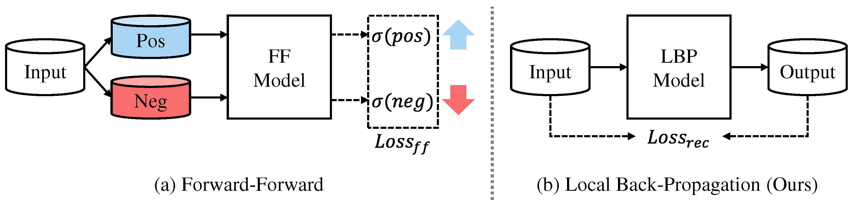
One of the key distinctions between the FF algorithm and our proposed LBP method lies in the design of the loss computation. As shown in Figure 2, FF requires the generation of positive and negative samples for each input, and computes a goodness score for each layer, where the goodness increases for positive samples and decreases for negative samples. This score, typically based on the squared norm of the activation vector, is then used to maximize the difference between positive and negative samples. Consequently, FF mandates custom data construction and specialized loss functions that deviate from standard deep learning practices.

In contrast, LBP adopts a more generalizable and modular approach. Each cell is trained independently using standard unsupervised learning objectives, such as reconstruction loss in AE or adversarial loss in GAN. Since the loss is computed locally within each layer, our method eliminates the need for label-conditioned sample engineering and allows compatibility with common input formats and standard loss functions like mean squared error or binary cross-entropy. This makes LBP more accessible and suitable for integration into conventional deep learning pipelines.

We propose the LBP learning approach, which leverages unsupervised deep learning models. By incorporating this strategy, we remove the input and loss function constraints previously present in FF, thus enabling the use of standard input formats and loss calculations commonly employed in general deep learning methods. Through this algorithm, our aim is to preserve the learning directionality characteristic of FF while ensuring compatibility with existing deep learning frameworks. We anticipate that this proposed method will prove highly effective in circumstances where the physical separation of layers poses challenges for applying BP.

Algorithm 1 outlines the detailed training procedure for the proposed Local Back-Propagation method. The training process consists of two main phases.

In the first phase (lines 1–13), each cell is trained independently in an unsupervised manner, sequentially from the first cell to the last. Each cell receives the latent representation output from the preceding cell as input, thus maintaining a forward sequential dependency. Within each cell, an unsupervised model, such as an Auto-Encoder, reconstructs the input data. The reconstruction loss is calculated independently per cell, and the cell’s parameters are updated accordingly. After training a cell, the learned latent representation is passed forward to serve as the input for the next cell, while the trained cell itself can be unloaded from GPU memory to optimize memory usage.

Algorithm 1: Local Back-Propagation (LBP) Training

Require:  Input data x, label y, number of cells C, learning rate $\eta$, number of epochs T Ensure:  Trained cell parameters $\{{\theta }_1,\dots ,{\theta }_C\}$ and classifier ${\theta }_{\mathrm{cls}}$ 1: for $c=1$ to C do 2:     Initialize parameters ${\theta }_c$ 3:     for $t=1$ to T do 4:         for all mini-batch $x_{\mathrm{batch}}$ do 5:            if using noise then 6:                $x_{\mathrm{batch}}\leftarrow x_{\mathrm{batch}}+ϵ$                   ▹ Add noise (e.g., Gaussian) 7:            end if 8:            $x_{\mathrm{batch}}\leftarrow$LayerNorm($x_{\mathrm{batch}}$) 9:            $z\leftarrow$Encoder($x_{\mathrm{batch}}$) 10:            $\widehat{x}\leftarrow$Decoder(z) 11:            ${\mathcal{L}}_l\leftarrow {\parallel x_{\mathrm{batch}}-\widehat{x}\parallel }^2$                     ▹ Reconstruction loss 12:            ${\theta }_l\leftarrow {\theta }_l-\eta ·{\nabla }_{{\theta }_l}{\mathcal{L}}_l$ 13:         end for 14:     end for 15:     Store z as input for cell $c+1$ 16: end for 17: Concatenate all latent vectors $z_1,z_2,\dots ,z_C$ into $z_{\mathrm{concat}}$ 18: Initialize classifier parameters ${\theta }_{\mathrm{cls}}$ 19: for $t=1$ to T do 20:     for all mini-batch $(z_{\mathrm{batch}},y_{\mathrm{batch}})$ do 21:         $\widehat{y}\leftarrow$Classifier($z_{\mathrm{batch}}$) 22:         ${\mathcal{L}}_{\mathrm{cls}}\leftarrow$CrossEntropy($\widehat{y},y_{\mathrm{batch}}$) 23:         ${\theta }_{\mathrm{cls}}\leftarrow {\theta }_{\mathrm{cls}}-\eta ·{\nabla }_{{\theta }_{\mathrm{cls}}}{\mathcal{L}}_{\mathrm{cls}}$ 24:     end for 25: end for

In the second phase (lines 14–21), once all cells have completed their unsupervised training, the latent representations produced by each cell are concatenated to form a combined feature vector. This combined representation is then used to train a supervised classifier. The classifier parameters are updated by minimizing a classification loss, such as the cross-entropy loss, using labeled training data.

To help readers better understand the training procedure in Algorithm 1, we summarize the meaning of all mathematical symbols used in

Table 1. Symbol definitions used in Algorithm 1.

Symbol	Definition
x	Input data
y	Ground-truth label
${\theta }_c$	Parameters of the c-th LBP cell (encoder and decoder)
${\theta }_{cls}$	Parameters of the final classifier
$\eta$	Learning rate
T	Number of training epochs
z	Latent vector output from encoder
$\widehat{x}$	Reconstructed input from decoder
$L_l$	Reconstruction loss of layer l ($\parallel x-\widehat{x}{\parallel }^2$)
$z_{\mathrm{concat}}$	Concatenation of all latent vectors
$\widehat{y}$	Output prediction of classifier
$L_{cls}$	Classification loss (cross-entropy)
$ϵ$	Added noise (e.g., Gaussian)

. This notation table provides concise definitions for the variables and parameters introduced in the LBP algorithm.

A key benefit of our LBP approach is its memory efficiency. Because each cell can be trained individually without simultaneously loading the entire network into memory, the proposed method enables training deeper networks or networks with larger parameters, even in resource-limited settings.

3.1. Architecture

The overall structure of our model is shown in Figure 1. The original data are fed into the first cell, and each cell performs unsupervised learning, similar to approaches used in Auto-Encoders or GANs, by attempting to reconstruct its input. This design is flexible and can be applied to any system capable of calculating a local loss independently in each cell. Although we focus on reconstruction-based models here, the approach can be extended to any method that produces latent vectors of a consistent size at each cell.

Figure 3 illustrates the basic form of a single cell using these models. In each cell, the encoder receives input data or latent vectors from the previous cell, compressing it into a lower-dimensional latent representation. The decoder attempts to reconstruct the original input from the latent representation, generating reconstruction data. The reconstruction loss between input data and reconstruction data is minimized independently in each cell, providing local supervision.

The unsupervised learning models we employ in this study include AE, DAE [25], CAE, and GAN. Figure 3a shows a cell using an AE, while Figure 3b depicts a DAE-based cell, where random noise is introduced into the input. Figure 3c presents a CAE cell, which uses a convolutional encoder and a transposed convolutional decoder. Figure 3d illustrates a cell incorporating a GAN structure, in which the generator is built like an AE, and the discriminator compresses both the real and decoder-produced (fake) data into one-dimensional vectors to judge authenticity.

Each unsupervised learning model is implemented with as few layers as possible for simplicity. We fix the latent vector size at half the size of the input for computational convenience. While there are no strict limits on the number of cells, if additional cells are needed and the latent vector size cannot be further reduced, we maintain the same latent vector size in subsequent cells.

The final classifier layer provides the model’s overall output. Unlike the cells, this layer is a standard fully connected layer (or potentially another type, depending on the task) and does not rely on unsupervised learning. It takes as input the concatenation of the latent vectors from all preceding cells.

To better illustrate the positioning of our proposed LBP method within the broader context of deep learning training strategies, we provide a comparative summary of its key properties relative to traditional BP and the FF algorithm.

Table 2. Comparison of back-propagation (BP), Forward-Forward (FF), and the proposed Local back-propagation (LBP) across core aspects such as training flow, input requirements, loss function types, memory efficiency, and compatibility with standard deep learning pipelines.

	BP	FF	LBP (Ours)
Training method	Forward–Backward	Forward-only	Forward–LocalBackward
Input format	Raw data	Positive/Negative	Raw data
Layer isolation	No	Yes	Yes
Memory efficiency	Low	High	High
Training stability	High	Low	Moderate
Loss function	General-purpose	Specialized	General-purpose
Compatibility	Yes	Limited	Yes

highlights the fundamental differences across core aspects such as training mechanics, input requirements, memory usage, and compatibility with conventional pipelines. This comparison clarifies how LBP inherits the forward-only advantage of FF while addressing its limitations through general-purpose loss functions and improved modularity.

3.2. Model Training

In models constructed using the AE series (Figure 3a–c), the encoder transforms the input data into a latent vector, and the decoder is then trained to reconstruct the input from this latent representation. During training, the encoder’s output latent vector from one cell is provided as input to the next cell.

In models that incorporate GAN (Figure 3d), the generator takes random noise as input. Within the generator, the encoder produces a latent vector, and the decoder subsequently generates fake data from this latent vector. The discriminator receives both real and generated data, learning to distinguish between the two. Through this process, the generator refines its ability to produce data that the discriminator deems authentic. After training, the encoder’s latent vector from the generator, using input from the previous cell, serves as the input to the subsequent cell.

In Figure 1c, the final layer in each model is trained to produce the desired outputs. Depending on the task, this may involve classification, regression, or generation. As with the other cells, the final layer is trained locally.

For input reconstruction tasks, we employ mean squared error as the loss function. When training the discriminator in GAN, binary cross-entropy is used. The final classification layer utilizes cross-entropy as its loss function. In all models, the AdamW [28] optimizer is applied, and ReLU [29] is used as the activation function.

To further stabilize training and enhance the generalization, layer normalization [30] is applied to every input of each cell. This step helps mitigate issues such as vanishing or exploding gradients, leading to more stable and efficient learning.

3.3. Layer-Wise Sequential Training and Memory Efficiency

Although our LBP algorithm allows each cell to be trained independently, this training process is inherently sequential. Each cell requires the output from the preceding cell as input, enforcing a forward-sequential dependency. This sequential nature means that cells cannot be trained in parallel. However, unlike conventional BP, which requires all cells’ parameters to be simultaneously loaded into GPU memory to compute global gradients, our method permits cells to be trained independently in sequence. Specifically, we load only one cell at a time into GPU memory, train it fully, then unload it before loading the next cell.

Consequently, our method significantly reduces peak memory usage, allowing models with many cells or larger parameters to be trained efficiently even on devices with limited GPU memory. This sequential but independent training structure is particularly advantageous for edge computing and federated learning scenarios, where computational resources and memory are constrained.

4. Experiments

Our primary goal in these experiments is not to achieve state-of-the-art classification accuracy. Instead, we aim to validate the feasibility and core characteristics of the proposed LBP. Specifically, we seek to demonstrate that LBP can serve as a practical alternative to back-propagation, particularly in resource-constrained environments. We also evaluate its comparative advantages over related methods, such as the FF algorithm. To this end, we emphasize fair and transparent comparisons against relevant baseline models, all implemented under identical and controlled experimental settings. This approach enables a balanced assessment of the trade-offs between performance, training stability, and computational efficiency.

4.1. Datasets

The datasets used in our experiments include MNIST [31], CIFAR10, and CIFAR100 [32]. MNIST consists of 10 labels, with 60,000 training samples and 10,000 test samples. CIFAR10, similarly, has 10 labels, with 50,000 training samples and 10,000 test samples. CIFAR100 includes 100 classes grouped into 20 superclasses, containing 50,000 training samples and 10,000 test samples. In this study, we did not employ any validation data.

4.2. Models

We conducted experiments using various baseline models, including SLP, MLP, and CNN models trained with BP, as well as our proposed LBP models. Specifically, we examined four types of LBP models as layers: Auto-Encoder LBP (AE-LBP), Denoising Auto-Encoder LBP (DAE-LBP), Convolutional Auto-Encoder LBP (CAE-LBP), and Generative Adversarial Network LBP (GAN-LBP). Throughout the experiments, we maintained consistent configurations for the optimizer, hidden dimensions, and the number of cells.

For the SLP model, a single fully connected layer was employed to produce outputs directly from the input data. In both MLP and FF models, each layer consisted of one fully connected layer followed by a ReLU activation function. AE-LBP, DAE-LBP, and GAN-LBP models used a single fully connected layer and ReLU activation within each encoder and decoder. In GAN-LBP, the discriminator was implemented with a fully connected layer and a ReLU activation to map the input into a hidden vector, followed by another fully connected layer to generate the final output.

In the CNN and CAE-LBP models, each layer incorporated a convolution, a ReLU activation, and a max pooling operation. For convolutional layers, we employed a kernel size of 3, a stride of 1, and a padding of 1, while max pooling utilized a kernel size of 2. In the CAE-LBP decoder, we applied transpose convolutions for reconstruction, using a kernel size of 2 and a stride of 2. When using MNIST, where the image width and height are 28, passing through two CAE-LBP layers reduces these dimensions to 7. Because 7 is an odd dimension, we used a convolution kernel size of 2 and a transpose convolution with a kernel size of 4 and a stride of 1 under these conditions.

4.3. Experimental Setup

In these experiments, we utilized the FF source code (https://github.com/loeweX/Forward-Forward (accessed on 8 June 2025)) implemented in PyTorch (version 2.1.0).

We employed the Weights and Biases (WandB) [33] hyperparameter tuning tool, known as Sweep, to train our models. Each experiment was repeated 10 times to assess performance variance. The batch size was fixed at 512 for all experiments. For MNIST, the maximum number of epochs was set to 100, and for CIFAR10, it was set to 200. The noise ratio for DAE-LBP was fixed at 0.2. Additionally, the hidden dimension for each model was set to 1024, and in LBP models, the hidden dimension was halved at each cell.

The hyperparameters explored for the SLP and MLP are as follows:

• Learning rate: [1 × 10⁻³, 1 × 10⁻⁵];
• Weight decay: [1 × 10⁻², 1 × 10⁻⁴].

The FF, AE-LBP, DAE-LBP, CAE-LBP, and GAN-LBP models underwent hyperparameter searches. We assigned different ranges of learning rates and weight decay values to the final classifier layer than those used for the preceding FF layers and cells, as the FF layers and cells generally required sufficiently low learning rates.

• FF layer and cell learning rate: [1 × 10⁻⁴, 1 × 10⁻⁶];
• FF layer and cell weight decay: [1 × 10⁻³, 1 × 10⁻⁵];
• Classifier layer learning rate: [1 × 10⁻³, 1 × 10⁻⁵];
• Classifier layer weight decay: [1 × 10⁻², 1 × 10⁻⁴].

For CNN and CAE-LBP models, the number of output channels in the first convolutional layer was configured so that it doubled with each subsequent convolutional layer.

• First convolution output channel size: 8, 16, 32, 64.

The SLP model’s hyperparameter search was performed once per dataset, followed by 10 runs to measure performance. For the other models, the number of layers was set to 2, 3, 4, or 5, and hyperparameter searches were conducted for each layer configuration, yielding a total of 40 performance measurements across all datasets.

When applying the FF learning method, each cell is trained independently. We therefore considered two training strategies. The first, termed sequence training, involves training each cell from the first to the final classifier layer within the same epoch. The second, termed separate training, involves fully training one cell for all epochs before moving on to the next cell. In this experiment, we compared the FF, AE-LBP, DAE-LBP, CAE-LBP, and GAN-LBP models under both sequence training and separate training approaches.

4.4. Experimental Results

Table 3. Best performances on the dataset. Bold values are the best of each model, italic values are the best of each learning method, and highlighted values are the best of our proposed models.

Dataset	Training Strategy	Layers	Baseline				Ours
			SLP	MLP	CNN	FF	AE-LBP	DAE-LBP	CAE-LBP	GAN-LBP
MNIST	Sequence	2	0.9274	0.9875	0.9921	0.9782	0.9689	0.9723	0.9791	0.9569
		3		0.9856	0.9942	0.9795	0.9706	0.9736	0.9821	0.966
		4		0.9875	0.9944	0.9751	0.9704	0.9722	0.9808	0.9581
		5		0.987	0.9951	0.9789	0.9713	0.9737	0.9793	0.9586
	Separate	2	0.9274	0.9875	0.9921	0.9687	0.9707	0.9679	0.9828	0.9621
		3		0.9856	0.9942	0.9674	0.9704	0.9710	0.9813	0.9604
		4		0.9875	0.9944	0.9694	0.9731	0.9721	0.9801	0.9598
		5		0.9870	0.9951	0.9700	0.9717	0.9729	0.9824	0.9598
CIFAR10	Sequence	2	0.3895	0.5439	0.6979	0.4886	0.4705	0.4691	0.5704	0.4467
		3		0.5393	0.7645	0.4713	0.4751	0.4474	0.5726	0.4394
		4		0.5364	0.7598	0.4751	0.4745	0.4573	0.5219	0.4542
		5		0.5205	0.777	0.462	0.473	0.4535	0.5394	0.4436
	Separate	2	0.3895	0.5439	0.6979	0.3308	0.4658	0.4539	0.5670	0.4420
		3		0.5393	0.7645	0.3508	0.4771	0.3788	0.5753	0.4410
		4		0.5364	0.7598	0.3939	0.4817	0.4772	0.6057	0.4573
		5		0.5205	0.777	0.3987	0.4813	0.4621	0.5705	0.4367
CIFAR100	Sequence	2	0.1606	0.2701	0.3916	-	0.2241	0.1633	0.1826	0.1669
		3		0.2543	0.4045	-	0.2394	0.216	0.2373	0.1523
		4		0.2378	0.3998	-	0.222	0.2033	0.2164	0.16
		5		0.2332	0.3931	-	0.2199	0.2166	0.219	0.1507
	Separate	2	0.1606	0.2701	0.3916	-	0.225	0.196	0.2164	0.1862
		3		0.2543	0.4045	-	0.2214	0.1911	0.2647	0.1854
		4		0.2378	0.3998	-	0.2369	0.1849	0.2333	0.1687
		5		0.2332	0.3931	-	0.2429	0.1634	0.2805	0.1756

presents the best performance results obtained from 10 runs of hyperparameter tuning for all experiments, including both sequence and separate training methods. All performances reported are measured in terms of accuracy. Across all experiments, the CNN model trained with BP consistently achieved the highest performance. On all datasets tested, both FF and LBP models, except for CAE-LBP, showed slightly lower performance than the MLP model. However, CAE-LBP consistently outperformed MLP. Additionally, LBP models generally demonstrated better performance than FF. Due to the requirement in FF that the number of input image pixels must match the number of labels, using FF on the CIFAR100 dataset, which has 100 labels, would result in a substantial loss of input image information. Therefore, we did not conduct FF experiments on the CIFAR100 dataset.

Under the sequence training approach, where each cell was trained for one epoch before moving to the next, FF achieved higher performance than most LBP models except for CAE-LBP. In contrast, when using the separate training approach, where the previous cells were fully trained up to the maximum number of epochs before training the next cell, LBP models generally outperformed their sequence training results and performed better than FF. Notably, when applying separate training on the CIFAR10 dataset, FF experienced a significant decrease in performance.

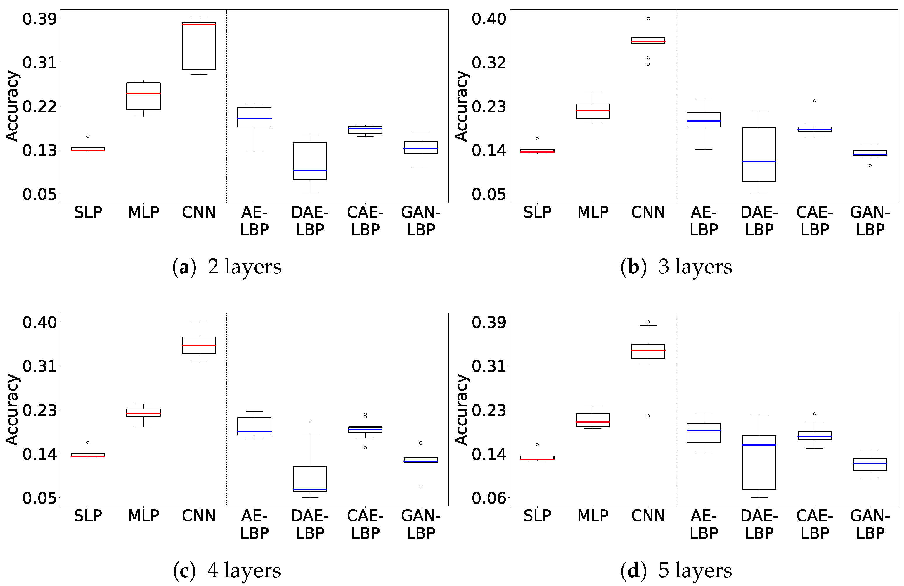
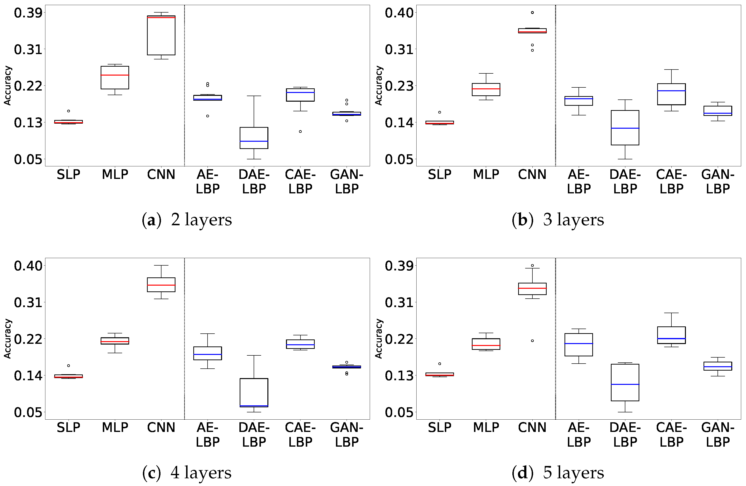
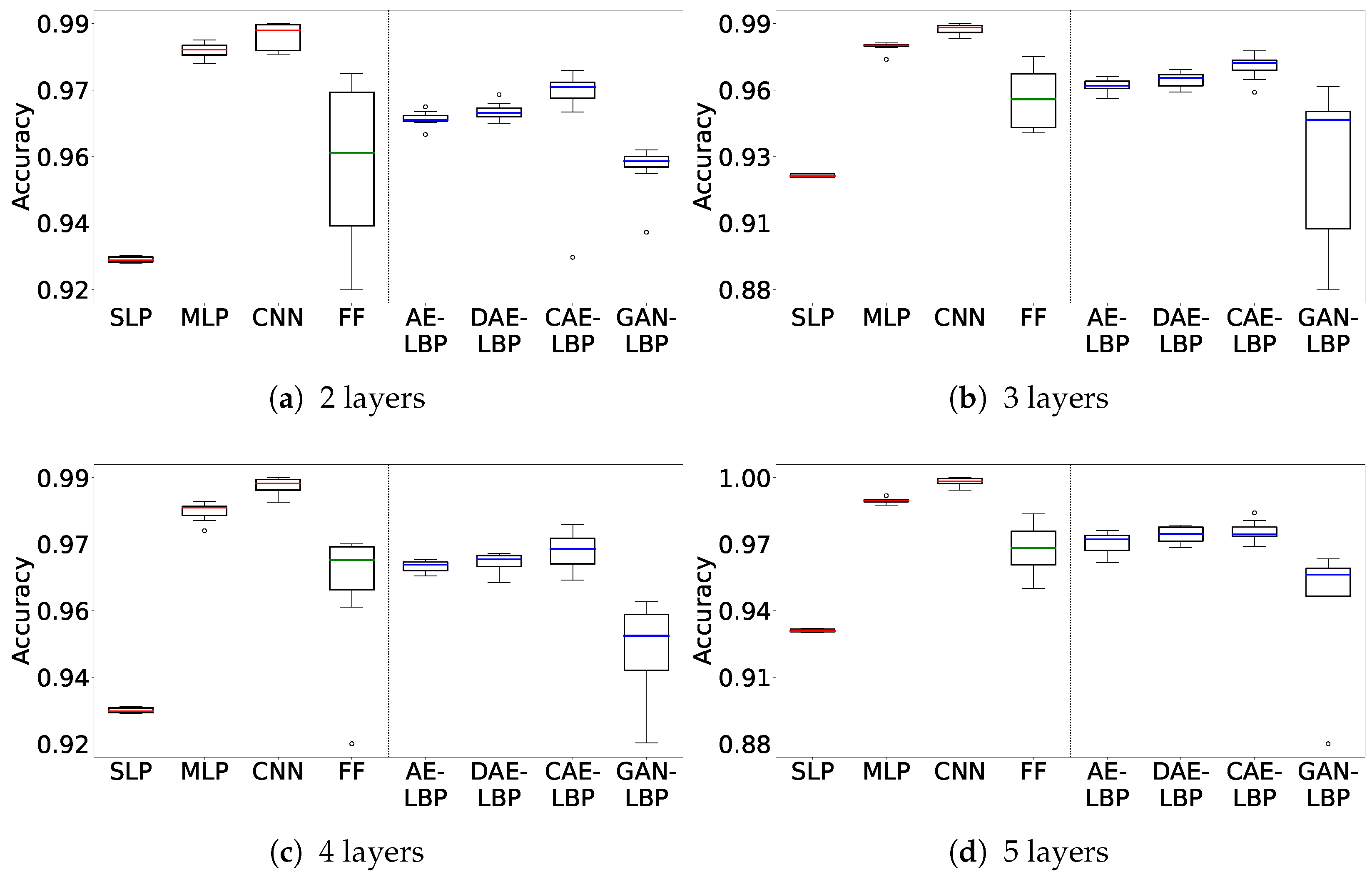
Figure 4 and Figure 5 show box plots of the results from the 10 hyperparameter tuning runs on the MNIST dataset for both sequence and separate training, covering the full range of experimental outcomes. The y-axis indicates accuracy, and the x-axis lists the models in order: SLP, MLP, CNN, FF, AE-LBP, DAE-LBP, CAE-LBP, and GAN-LBP. The circular points represent outliers, and the colored line inside each box denotes the median value. Each box extends from the 25th to the 75th percentile of the measured values.

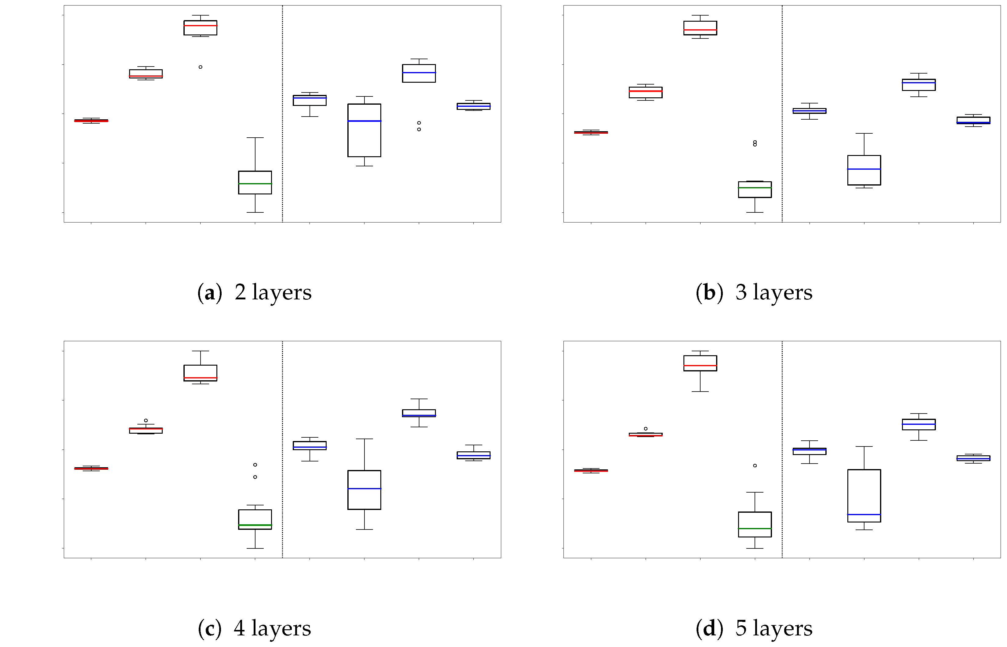
Figure 4 shows the sequence training results. Except for FF and GAN-LBP, most models exhibit stable performance distributions. Figure 5 shows the separate training results, where FF’s performance distribution is notably unstable.

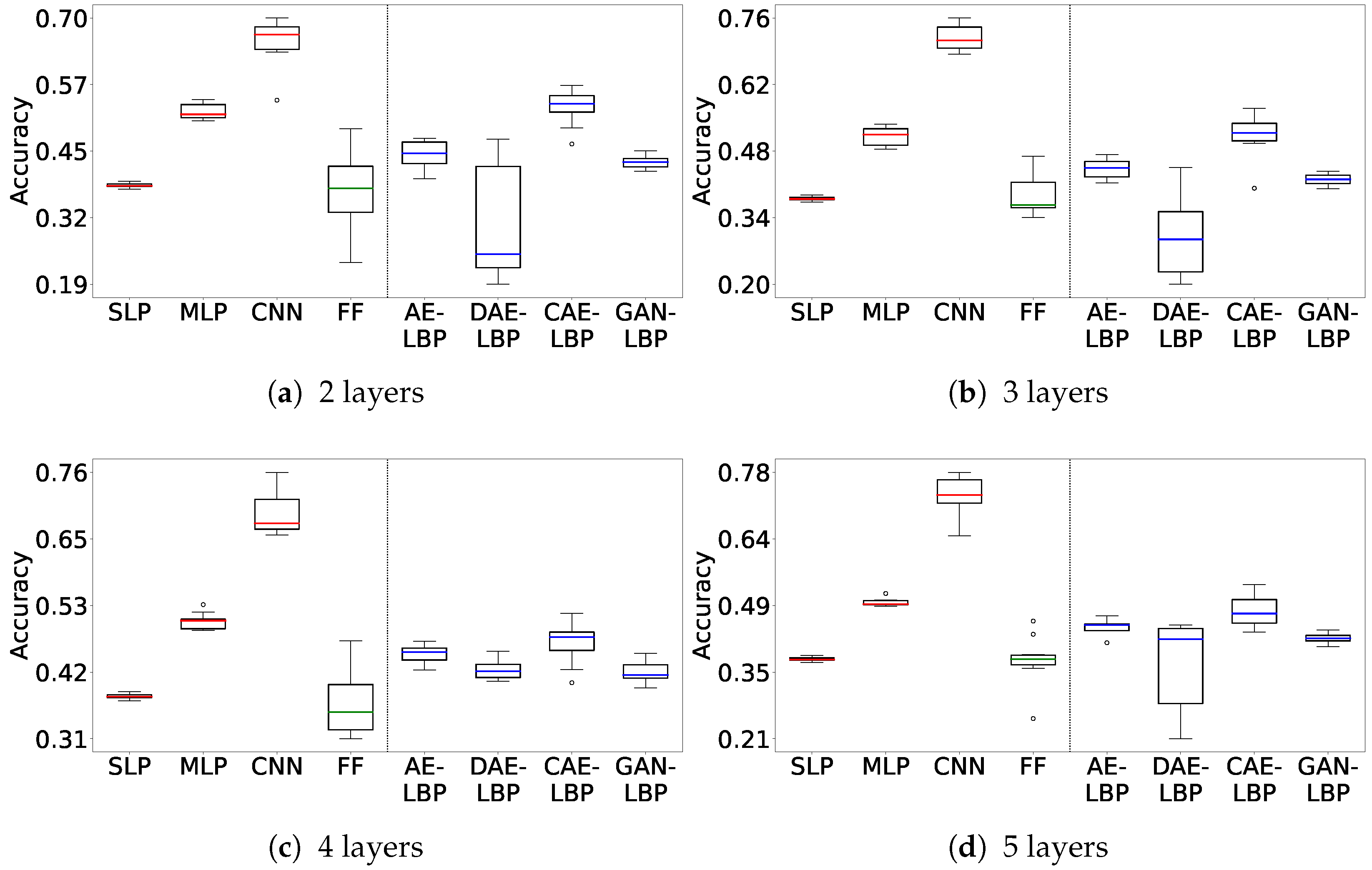
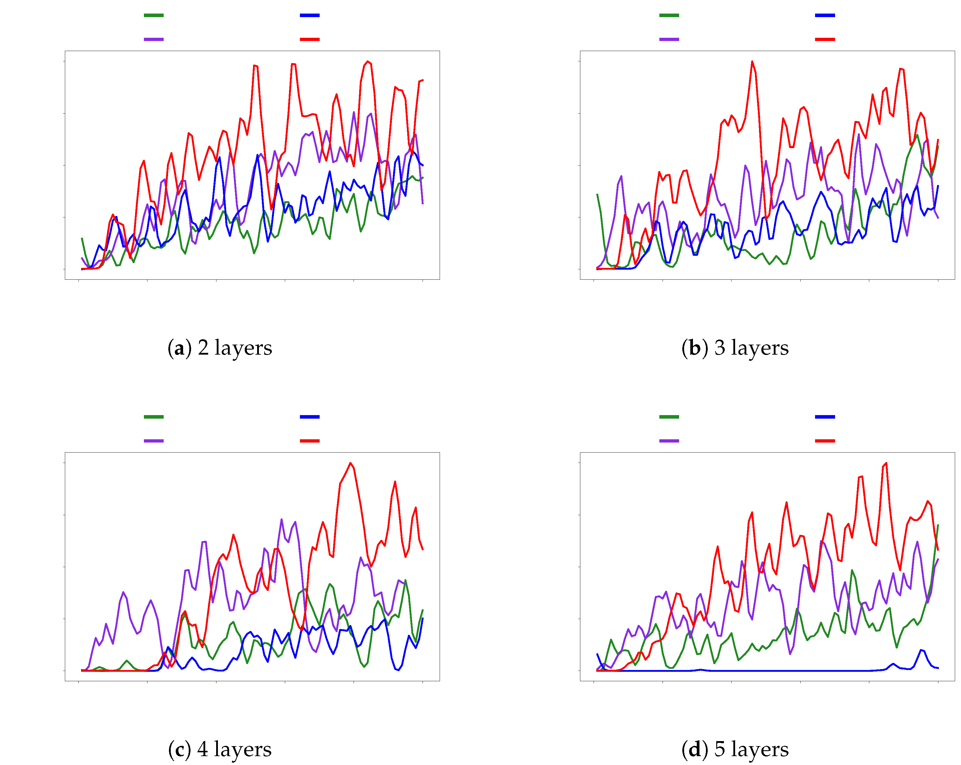
Figure 6, which shows the sequence training results for CIFAR10, indicates a broader performance range compared to MNIST. Notably, FF and DAE-LBP display unstable distributions. Figure 7, presenting the separate training results for CIFAR10, similarly shows that FF and DAE-LBP remain unstable. In contrast, GAN-LBP demonstrates more stable performance in separate training on CIFAR10 than it did on MNIST.

As shown, the FF model exhibits highly unstable performance across both datasets, especially on CIFAR-10, where its accuracy is both low and inconsistent. This suggests that despite using a similar number of parameters, the structural limitations of FF make it unsuitable for learning from datasets with higher information complexity.

In contrast, the proposed LBP variants show relatively stable performance on MNIST. On CIFAR-10, however, some variants display signs of instability. In particular, DAE-LBP and GAN-LBP tend to be more sensitive and perform worse, which may indicate that they are more vulnerable to noise. Additionally, we observe that the separate configuration shows more stable trends compared to the sequence setting. This suggests that when each cell is trained independently, the stability of earlier cells is crucial for the successful training of subsequent layers.

Nevertheless, our method also shows a general decrease in performance as the task complexity increases. This indicates that further improvement is needed to enhance the capacity of the model to capture and propagate richer representations across layers, especially for more challenging datasets such as CIFAR-10.

The performance on the CIFAR100 datasets can be found in Appendix A.

4.5. Application in Federated Learning

We conducted federated learning experiments to validate the practicality of our proposed method. Using the MNIST, CIFAR10, and CIFAR100 datasets, we compared the performance of MLP and CNN models with AE-LBP and CAE-LBP, which performed favorably among the proposed models. In total, we created 100 client models and ran 100 training rounds, randomly selecting 10 clients each round. At the end of each round, we updated the global model’s weights using Federated Averaging [34], which averages the weights of the selected 10 clients. The updated global model’s weights were then shared with all clients. In these experiments, the LBP cell was structured as an encoder–decoder, but to reduce communication costs and avoid reconstructing the input data, only the encoder weights were transmitted.

In federated learning with 10 clients, the AE-LBP model (7,889,572 parameters) required 1228 MB of GPU memory, and the CAE-LBP model (12,232,103 parameters) required 1872 MB. In comparison, the MLP model (8,497,252 parameters) required 1304 MB, while the CNN model (6,373,092 parameters) required 3630 MB. These results demonstrate that the proposed LBP-based models operate with lower memory overhead than conventional architectures. In addition, since LBP models allow each layer to be trained independently, memory is only needed for a single layer at a time. On the other hand, models trained with back-propagation must load and update all layers simultaneously, resulting in much higher memory usage. Therefore, the reported memory usage for LBP models represents a conservative upper bound. In practice, when layers are processed sequentially or in a pipelined manner, the actual memory consumption can be significantly lower. This advantage becomes more significant as model size increases, making the proposed approach well suited for edge computing and federated learning environments with limited computational resources.

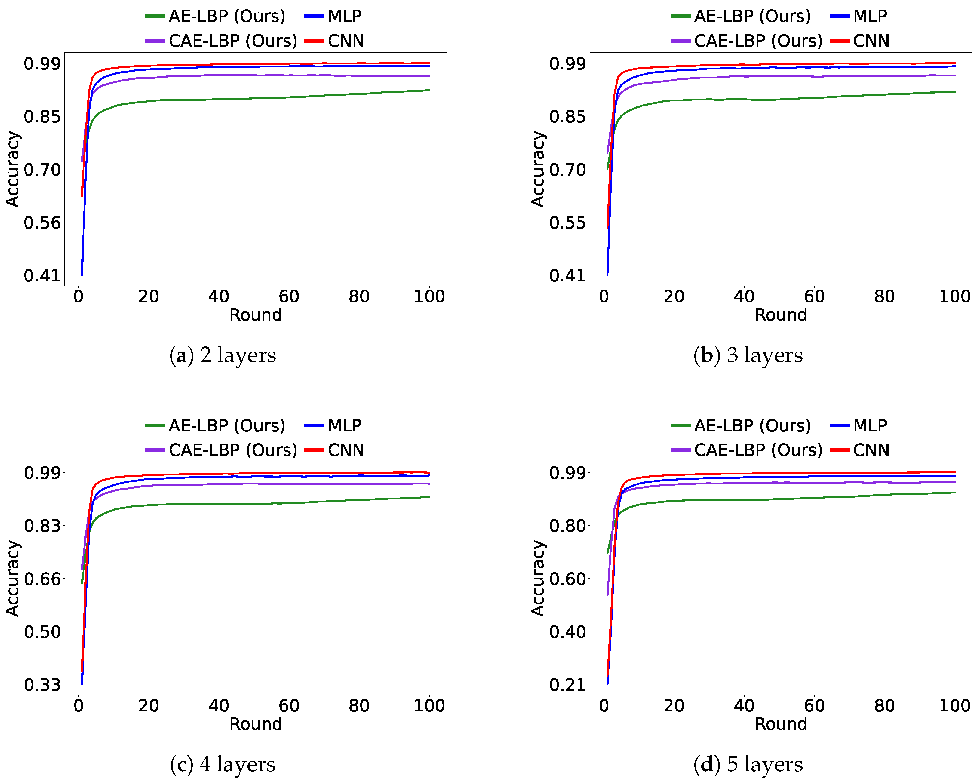
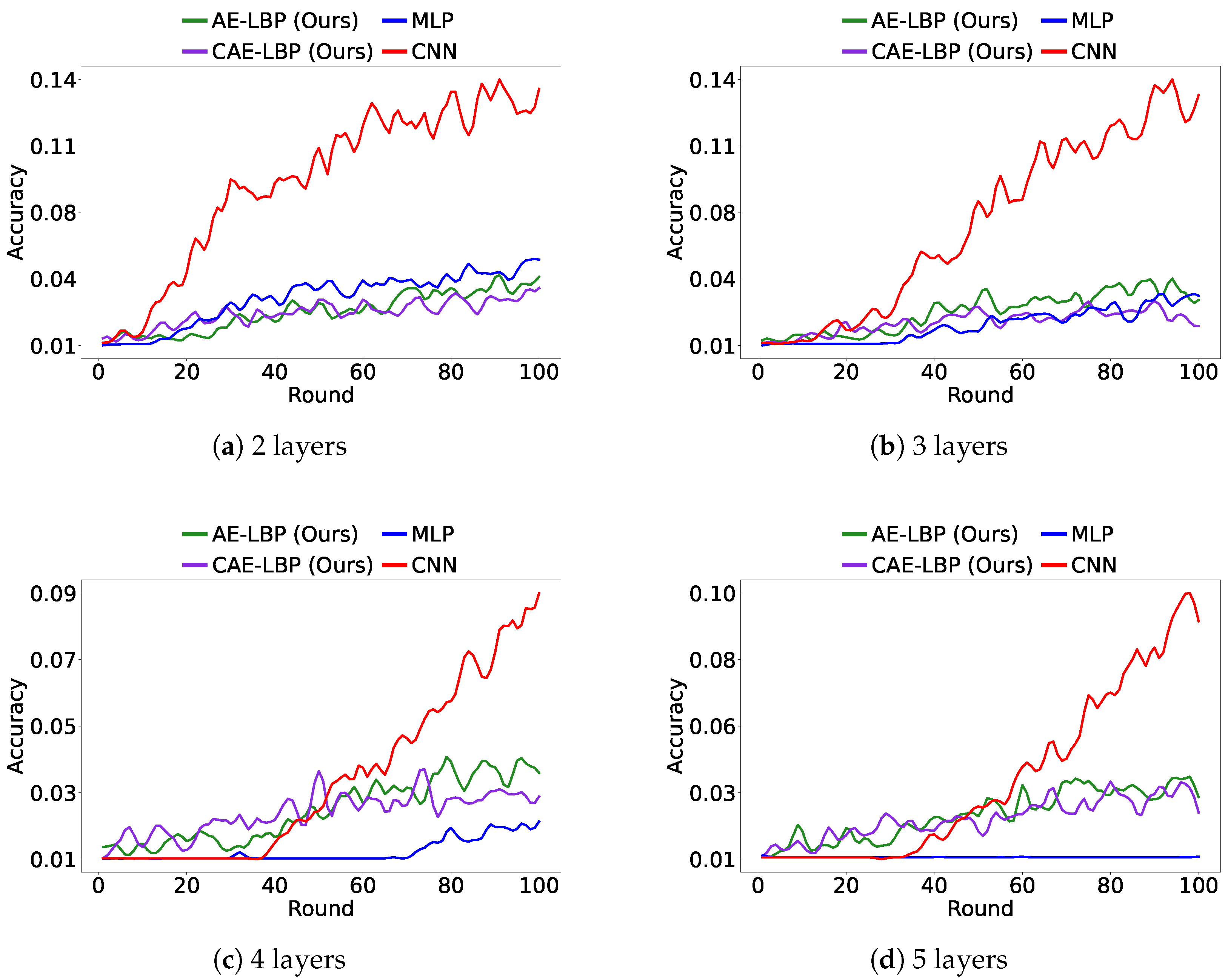
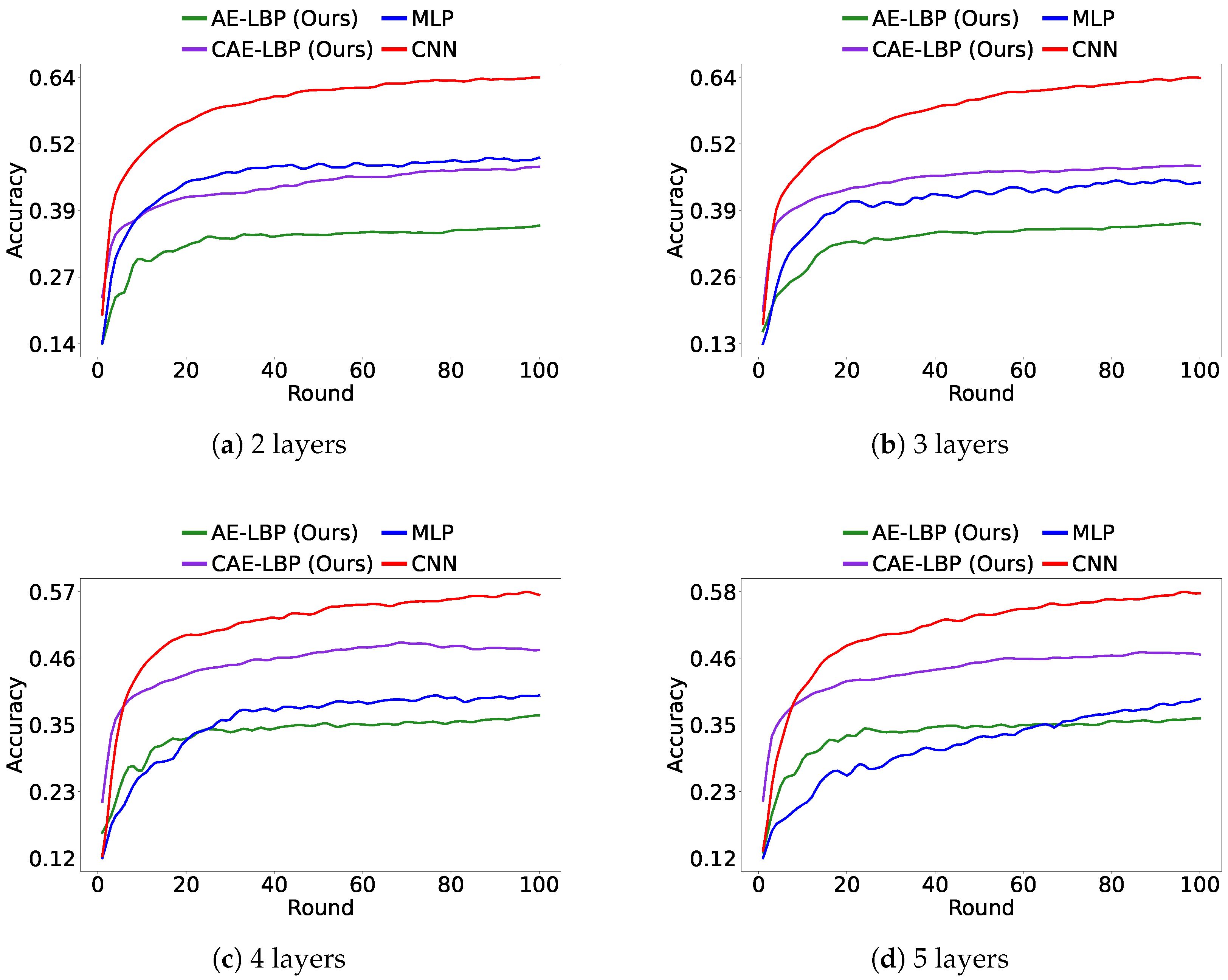
Figure 8 shows the accuracy of the global model after 100 rounds. While MLP outperformed AE-LBP and CAE-LBP on MNIST, as the data became more complex, AE-LBP and CAE-LBP showed better results. Furthermore, the performance of CNN models in Figure 8 indicates that simply increasing the size of the model does not guarantee improved results. These findings confirm the practicality of our approach and suggest potential for further improvements.

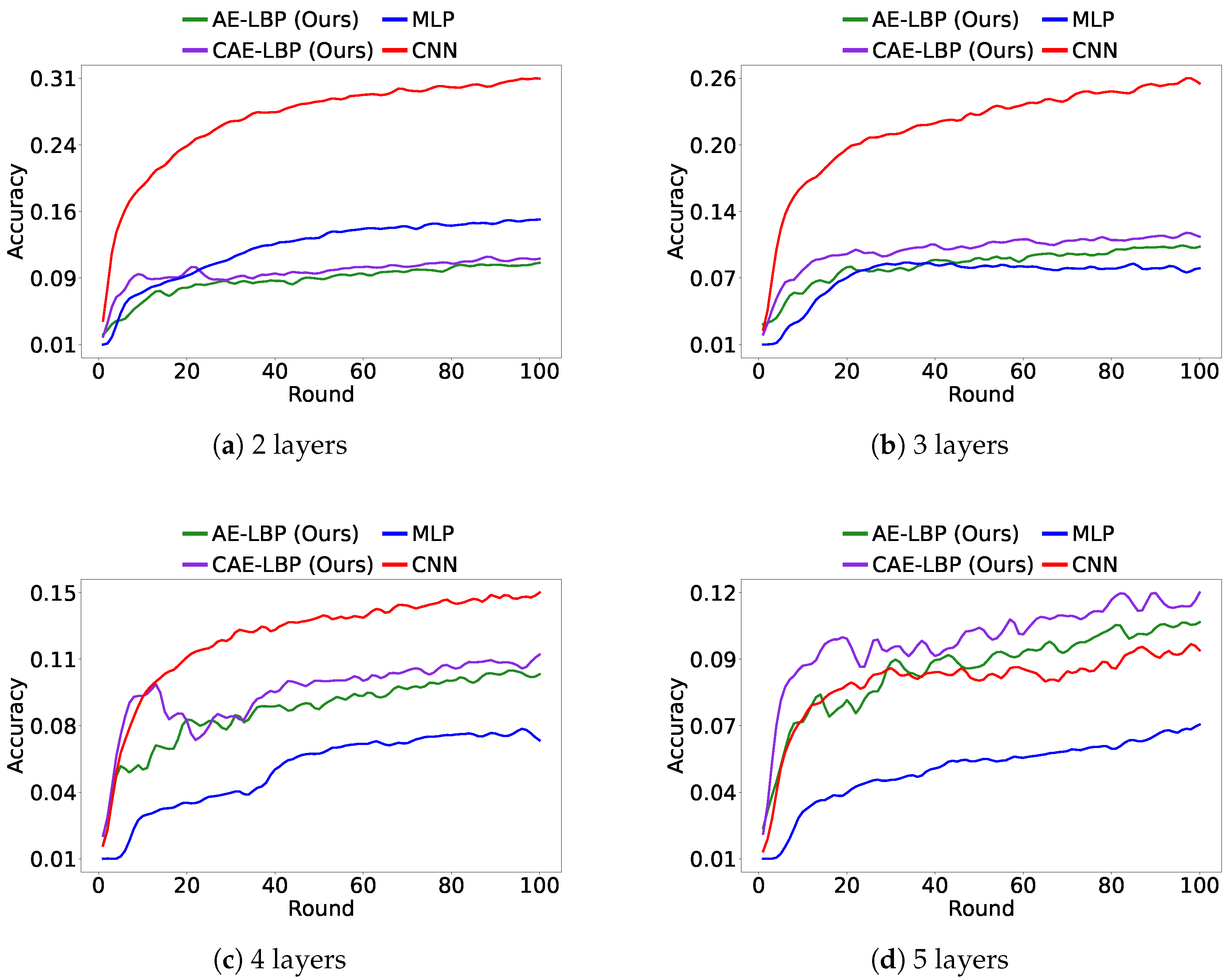
Figure 9 shows the results of federated learning experiments conducted with independent and identically distributed (IID) data, while Figure 10 and Figure 11 show results under non-IID data conditions. The datasets were structured so that at most 20% of the total labels could be selected at any given time, and all other experimental settings remained the same. Due to the randomness in data distribution, some learning scenarios were more challenging. However, overall, LBP models generally performed better than the MLP model.

4.6. Training Time Analysis

To evaluate the computational efficiency of LBP variants compared to traditional models, we measured the training time per epoch on the MNIST dataset. Each model was trained for one epoch, and the process was repeated five times to ensure consistency. The average training times (in seconds) are reported in

Table 4. Average training time per epoch (in seconds) on MNIST dataset (5 epochs).

Epoch	MLP	CNN	FF	AE-LBP	DAE-LBP	CAE-LBP	GAN-LBP
1	1.1446	1.8507	1.7861	7.2096	6.9589	1.8202	5.6002
2	0.7457	0.7409	1.3069	6.7662	6.8460	0.7384	5.1235
3	0.7499	0.7389	1.3014	6.6913	6.7954	0.7408	5.0654
4	0.7326	0.7360	1.2830	6.7360	6.8485	0.7392	5.1066
5	0.7530	0.7374	1.2985	6.7304	6.8335	0.7403	5.0608
Avg.	0.8252	0.9608	1.3952	6.8267	6.8564	0.9558	5.1913

.

As shown, LBP variants based on Auto-Encoders (AE-LBP and DAE-LBP) exhibit significantly longer training times due to the reconstruction process, while convolution-based CAE-LBP achieves a favorable trade-off between speed and performance. Notably, the CAE-LBP model maintains a low computational overhead similar to MLPs, while being substantially more efficient than AE-LBP and DAE-LBP.

In contrast, GAN-LBP requires additional computation for adversarial objectives, leading to moderately high training costs. FF itself demonstrates time efficiency close to MLP, but less efficient than CNN due to additional forward passes.

These findings confirm that while certain variants of LBP incur higher costs, others (e.g., CAE-LBP) maintain competitive training time, making them suitable for constrained environments.

5. Discussion

This study demonstrates that the proposed LBP method offers a viable alternative to BP by enabling deep learning without the need for backward passes. By extending the FF framework with layer-wise unsupervised learning, LBP eliminates the need for specialized inputs and non-standard loss functions, thereby addressing a key limitation of the original FF algorithm. Our results show that LBP achieves greater training stability than FF and enables practical application using standard data formats and objectives.

In terms of performance, the proposed LBP models consistently outperform SLPs, and in some configurations such as CAE-LBP and AE-LBP, they also surpass MLPs trained with BP, particularly in federated learning settings. These results suggest that local unsupervised training can still facilitate meaningful information propagation between layers, even in the absence of global gradients.

However, LBP generally shows lower performance than CNNs trained with BP, especially on complex datasets like CIFAR-100. We acknowledge this limitation. We believe that the relatively low performance stems from the local nature of training in LBP. Because each layer is trained independently, the model may struggle to capture sufficient semantic depth and inter-layer coherence. While BP enables multi-layer optimization through chained gradients, which can be seen as multiplicative in nature, LBP accumulates representational knowledge in an additive manner. This difference may lead to suboptimal parameter usage and reduced model expressiveness across layers.

An important finding from our federated learning experiments is the notable difference in performance scaling between CAE-LBP and AE-LBP as model depth increases. Specifically, while AE-LBP exhibited diminishing returns with the addition of more layers, CAE-LBP consistently demonstrated improved accuracy with deeper architectures.

We hypothesize that this trend arises from the inherent advantages of convolutional operations in capturing hierarchical spatial features. Each CAE-LBP cell serves as an effective local feature extractor, progressively constructing more abstract and informative representations from the outputs of preceding layers. The local reconstruction objective further encourages each cell to retain and refine essential spatial information before forwarding it to the next stage. In contrast, AE-LBP relies on fully connected layers that require flattening the input, which can lead to a loss of spatial structure and thus limit the benefits of increased depth.

Additionally, some LBP variants, such as DAE-LBP and GAN-LBP, displayed unstable training behavior, likely due to their sensitivity to injected noise or adversarial objectives. This highlights the importance of model selection and configuration when applying LBP to different tasks. These observations suggest that the proposed LBP framework is particularly well suited for convolutional architectures, and highlight its potential for scalable and efficient training of deep vision models in distributed learning environments.

From a practical standpoint, among the LBP variants, CAE-FF shows a balance between speed and performance, but other methods introduce a moderate increase in training time per epoch due to local reconstruction at each layer. However, this overhead is offset by significantly improved memory efficiency. Since each layer is trained independently and sequentially, the model can be trained with only one layer loaded into GPU memory at a time. This enables training of deep models in memory-constrained environments, such as edge devices or federated systems. Nonetheless, communication and coordination in federated settings remain open challenges.

In summary, LBP bridges a gap between biologically motivated algorithms and practical deep learning. While it cannot fully replicate the performance of BP, it offers a scalable and resource-efficient alternative suitable for certain deployment scenarios. Future improvements may include hybrid training strategies, enhanced reconstruction techniques, or lightweight inter-layer coordination to further close the performance gap while preserving the benefits of local training.

6. Conclusions

This study was motivated by the long-standing challenge of developing alternatives to the back-propagation algorithm that are both biologically plausible and resource-efficient. Although the Forward-Forward algorithm offers a promising direction, its reliance on handcrafted input samples and non-standard loss functions, as well as its training instability, has limited its practical applicability.

To address these limitations, we proposed the Local Back-Propagation framework, which employs independent, layer-wise unsupervised learning in place of the original Forward-Forward mechanism. This design eliminates the need for specially constructed positive and negative samples and allows the use of standard input formats and loss functions. Furthermore, it significantly improves training stability while maintaining compatibility with conventional deep learning pipelines.

Experimental results confirmed the effectiveness of the proposed approach, demonstrating competitive performance compared to standard MLP models and highlighting its notable memory efficiency. This advantage makes LBP particularly suitable for deployment in resource-constrained or decentralized environments such as federated learning.

For future work, we aim to reduce the performance gap between LBP and end-to-end trained models by exploring hybrid learning strategies that incorporate minimal global coordination. Additionally, we plan to investigate advanced unsupervised objectives within individual LBP cells and validate the proposed method on real-world edge devices to further evaluate its practical utility.