NRNH-AR: A Small Robotic Agent Using Tri-Fold Learning for Navigation and Obstacle Avoidance

Abstract

We propose a tri-fold learning algorithm, called Neuroevolution of Hybrid Neural Networks in a Robotic Agent (acronym in Spanish, NRNH-AR), based on deep reinforcement learning (DRL), with self-supervised learning (SSL) and unsupervised learning (USL) steps, specifically designed to be implemented in a small autonomous navigation robot capable of operating in constrained physical environments. The NRNH-AR algorithm is designed for a small physical robotic agent with limited resources. The proposed algorithm was evaluated in four critical aspects: computational cost, learning stability, required memory size, and operation speed. The results obtained show that the performance of NRNH-AR is within the ranges of the Deep Q Network (DQN), Deep Deterministic Policy Gradient (DDPG), and Twin Delayed Deep Deterministic Policy Gradient (TD3). The proposed algorithm comprises three types of learning algorithms: SSL, USL, and DRL. Thanks to the series of learning algorithms, the proposed algorithm optimizes the use of resources and demonstrates adaptability in dynamic environments, a crucial aspect of navigation robotics. By integrating computer vision techniques based on a Convolutional Neuronal Network (CNN), the algorithm enhances its abilities to understand visual observations of the environment rapidly and detect a specific object, avoiding obstacles.

1. Introduction

The progress of Artificial Intelligence (AI) has brought about a revolution in several fields, including mobile robotics. Traditionally, mobile robotics heavily relied on conventional control systems, which, although effective, had inherent limitations. These systems required extensive programming and adapted to changing environments or unforeseen tasks. Furthermore, their human factor often played a crucial role in accidents in complex or dangerous settings, as limitations in perceptive, decision-making, and physical capabilities can lead to errors. This highlights the need for more robust and adaptable solutions for navigating hazardous or inaccessible environments. The DRL, a subset of AI, offers a promising alternative by enabling robots to learn and improve through interactive engagement with their environment [1,2,3,4]. This approach has significant potential for enhancing adaptability and overall performance in robotics.

Unlike traditional DRL approaches, the proposed method (NRNH-AR) incorporates pre-training stages based on SSL and USL to reduce training time and computational load during the DRL phase. NRNH-AR is a novel DRL-based algorithm specifically designed for deployment on a small physical robot with limited computational resources. This approach offers advantages in terms of adaptability, computational efficiency, and the ability to learn with limited data, making it well-suited for real-world applications where robots must operate in dynamic and unpredictable environments. Our primary objective is to develop and validate a novel DRL-based algorithm in a small autonomous physical robot designed for real-world navigation in narrow or complex environments. Because the robot is small, it must operate with limited resources, such as a small memory size and low computation capacity. The NRNH-AR algorithm optimizes these resources using tri-fold learning phases.

Small-sized robots have been developed for various applications, such as exploration and rescue in disaster regions, where human rescuers cannot enter due to narrow space and dangerous situations [5]. In the agricultural field, due to a lack of workers, several navigation robots were developed for purposes such as crop health monitoring and soil moisture assessment [6]. Due to narrow paths in the greenhouses, the size of the robots must be small enough to function properly. In [7], a small cleaning robot, which detects and removes sharp metal objects from the road, was developed, and the authors of [8] developed a small robot to detect mine holes. The size of the robot was adapted to the diameters of the holes. The robots used in [9] are categorized as small robots, the purpose of which is to avoid obstacles efficiently. The sizes of these small robots range from approximately 4 cm × 2 cm × 1 cm to 40 cm × 30 cm × 10 cm, depending on the application and the environment where the robot operates. Almost all robots use the simultaneous localization and mapping (SLAM) algorithm to understand their environment.

The implementation of reinforcement learning algorithms in robotics has been the subject of extensive research [10,11,12,13,14,15,16,17,18,19,20,21,22]. These studies have explored various applications, including the active classification of moving targets using control policies learned in realistic environments [13,14,15,16,17]. For instance, Ref. [18] presents a DRL approach with a fuzzy attention mechanism and heterogeneous graph neural networks (FAM HGNN) to address obstacle avoidance in robotics environments. Similarly, Ref. [19] leverages LiDAR sensors for obstacle evasion and environmental understanding during navigation. In the field of autonomous robot navigation, works such as Refs. [8,20,21] have developed DRL algorithms to enhance decision making, enable active exploration, adapt to changing conditions, and optimize efficiency and safety, even in crowded environments. Another study [22] focuses on predicting pedestrians using visual sensors and neural networks, providing an innovative solution for robot navigation in dense crowds. Recent advances in obstacle avoidance have significantly enhanced mobile robot navigation. Yunchao et al. (2024) presented a comprehensive analysis of global and local obstacle avoidance algorithms, highlighting trade-offs in convergence and computational efficiency [23].

Upon analyzing the six previous works [9,18,19,20,21,22], it is evident that five of them primarily focused on software or algorithm development, demonstrating an efficiency of over 80%. However, it is important to note that none of these works were tested in real operating environments, which limits the ability to assess their true effectiveness and applicability. Conversely, the work presented in [20] underwent physical evaluation, providing more tangible performance data, albeit with an efficiency of 60%. It is crucial to recognize that, while these works, implemented on high-capacity hardware with almost no limited memory space, can solve the robust testing environment, the practical transferability of these algorithms may encounter several limitations. The main limitations are limited energy problems, limited processing capacity, and limited memory space.

By harnessing the power of DRL in physical robotics, the NRNH-AR algorithm enhances data analysis efficiency and enables robots to exhibit greater adaptability. Assuming these outcomes, the principal contributions of this paper are as follows:

• The development of a small autonomous physical robot capable of exploring narrow spaces that humans cannot enter. However, the size of the robot is scalable depending on applications.
• The reduction in the time steps required to explore the static and/or dynamic environments, with three learning phases, the SSL phase, the USL phase, and the DRL phase, fused in this order.
• The use of the tri-fold learning design optimizes resource usage, such as memory space and computational cost, which is an important factor for the small autonomous physical robot.

The rest of the paper is organized as follows. Section 2 describes the materials and methods used in the research, in which the three learning phases and the design of the robotic agent are described. Section 3 presents the experiments realized, and Section 4 provides the results obtained from the experiments. A complete analysis of the performance of our algorithm is included, and the results of other researchers are compared. Finally, Section 5 presents the conclusions of the study, summarizes the results obtained, identifies the limitations of the proposal, and outlines future research directions.

2. Materials and Methods

This section details the architecture of the proposed algorithm, whose preliminary version was presented in conference paper [24]. The first subsection describes the global model of the proposed algorithm, which consists of three learning phases, each of which is described in the following subsections. Then, the design architecture is presented, and the characteristics of the components used, and the robotic agent, are detailed.

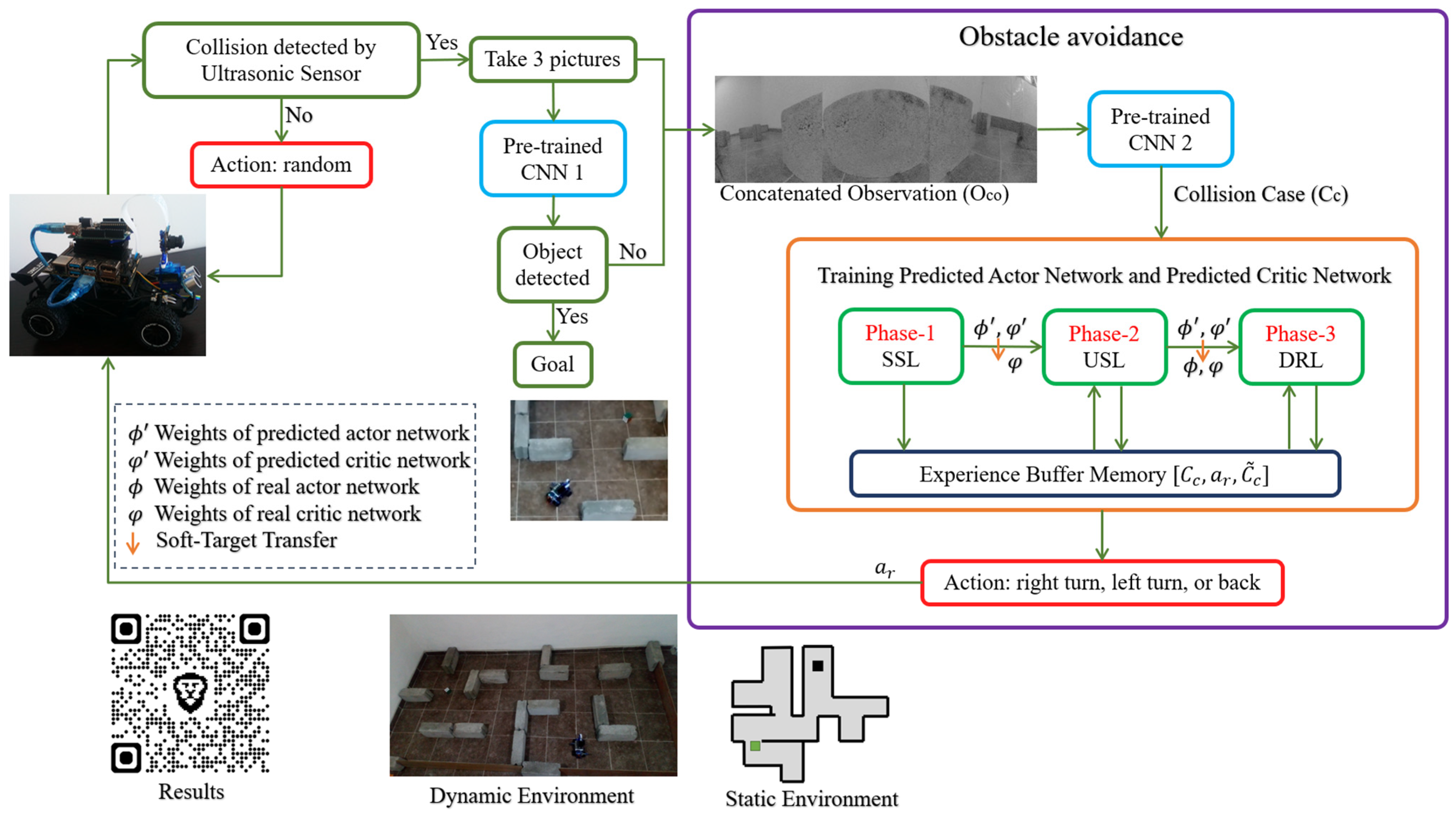
2.1. Overview of the NRNH-AR Algorithm

The overview of the NRNH-AR algorithm is shown in Figure 1. The robot agent uses two sensors, a camera and an ultrasonic sensor, HC-SR04, collocated in front of the robot agent, as shown in Figure 2. While the robot agent does not find any obstacle ahead, it realizes an action randomly selected within (forward, right turn, left turn, back). The agent halts if the ultrasonic sensor emits an active signal, indicating an obstacle to its front. Then the agent captures three images with the camera at angles of 15°, 90°, and 165°, as shown in Figure 2, considering that 90° is the robot looking straight ahead. These three images are introduced sequentially to pre-trained CNN 1, to determine whether one of the three images is the target object. If yes, the agent achieves its goal; otherwise, the robot agent realizes the obstacle avoidance action using the three previous images, concatenating them to form a single image, called a Concatenated Observation (O_co), which is used as an input for a second pre-trained CNN (CNN 2) to understand the collision state and train the actor and critic networks that predict the best action with the highest quality in the current state of the agent.

To optimize the use of the limited resources of the small robot agent, we have structured the training process into three distinct phases: SSL, USL, and DRL. The objective of all learning phases is to train two networks, which are a predicted actor network and a predicted critic network. These two networks are fully connected neural networks with two hidden layers. Three learning phases share the networks’ connection weights. Instead of training these networks directly using one of the DRL algorithms, such as DQN and TD3, we use triple learning phases composed of SSL, USL, and DRL to reduce computational costs and required memory space.

During the SSL phase, the primary objective is to quickly gain experience by receiving clear instructions on the actions it should perform. This is accomplished by considering the input image of the environment captured by the camera and the signal from the ultrasonic sensor. By learning from labeled examples generated by the row image and the sensor signal, the agent can make informed decisions and update the connection weights of networks. In the USL phase, the supervisor’s decisions are replaced by a parallel neural network system, like TD3, but without the reward concept. This system calculates two actions based on the observed collision case and the future collision case as input data, using twin actor networks, and evaluates each quality value using critic networks. This approach allows the agent to learn intrinsic patterns and features of the environment without relying on labels or direct supervision. During this phase, the connection weights of all networks, two actor networks and two critic networks, are further updated.

In the final DRL phase, the agent builds upon the knowledge acquired in the previous two phases, SSL and USL, through the updated connection weights of networks, and introduces the concepts of rewards. The agent also considers the time it takes to achieve its goal. Therefore, each time step until the agent finds the object causes a negative reward. Through direct interaction with the environment, the agent learns and adjusts its actions based on the rewards received. This continuous learning process causes the agent’s behavior to improve and adapt over time.

2.2. Vision-Based Environmental Understanding

The CNNs play an important role in physical robot navigation, enabling them to understand environmental information and perform their assigned task. In the proposed scheme, the robot agent contains two CNNs, CNN 1 and CNN 2, as shown in Figure 1. CNN 1 is pre-trained offline for detecting a specific target object, and CNN 2 is trained during navigation for understanding the environment. For CNN 1, we perform transfer learning in the pre-trained MobileNet V3 [25], introducing several images of the target object with different scales and viewpoints. This CNN can be replaced by any lightweight CNN according to the hardware limitations.

Regarding CNN 2, as shown in Figure 3, the NRNH-AR algorithm starts training a shallow CNN, follows sequential progression from SSL to USL, and finally reaches DRL. As mentioned earlier, the training of CNN 2 begins with creating a database composed of a concatenated image $O_{co}$; one example of this can be observed at the top of Figure 3.

In Figure 3, ε represents the current amount of environmental information (database size) and the threshold value η is the minimum amount of data necessary to train CNN 2; its importance lies in avoiding ineffective computational expenditure due to a lack of information. If ε exceeds η, it indicates that there are sufficient images to train CNN 2. Otherwise, additional images are continuously added to the database. The loss value of CNN 2 decreases oscillatory as the database size increases, but the training time and energy consumption increase with the database size. Considering the relation between these two conflicting issues, we select the database size when the training loss value of CNN 2 reaches less than 1.0 the minimum database size η, which is equal to 623.

In the CNN 2 training process, grayscale images in the size of 150 × 150 are introduced as input data, and four probability values, corresponding to four classes, are output. These four classes correspond to four collision cases captured by the ultrasonic sensor, as shown in

Table 1. Four collision classes that CNN 2 classifies $O_{co}$.

Collision Case	Class Case (${\mathit{C}}_{\mathit{c}}$)
[0 1 0]	1
[0 1 1]	2
[1 1 0]	3
[1 1 1]	4

. It is worth mentioning that the other four possible cases, such as [1 0 1], [0 0 0], etc., are not included as collision cases, because these do not present any collision in front of the agent, allowing the agent to move ahead. We denominate the output of CNN 2 as $C_c$ for further use in the subsequent learning phases.

.

The architecture of CNN 2, which is trained using 623 concatenated observation images, $O_{co},$ with the Adam optimizer to minimize the Categorical Cross Entropy loss function, is provided in

Table 2. CNN 2 architecture.

Layer Name	Parameters
Input	150 × 150 × 1
Conv1	3 × 3 × 32
Maxpool 1	2 × 2
Conv2	2 × 2 × 64
Maxpool 2	2 × 2
Fc1/ReLU	120
Fc2/SoftMax	4

. The number of epochs required is 50. This architecture is selected as the optimum after several analyses of the performance of the subsequent learning phases. The number of epochs is relatively small because the capability of a robotic agent to avoid obstacles can be improved through SSL, USL, and DRL.

Once CNN 2, whose weights are fixed for use in the subsequent phases, has been trained, the study proceeded with the SSL, USL, and DRL phases, in that order.

2.3. Self-Supervised Learning Phase

In this phase, the ultrasonic sensor data and pre-trained CNN 2 are used. If the physical robot agent detects an obstacle to its front receiving the active ultrasonic sensor signal, then the concatenated observation $O_{co}$ is taken by the agent’s camera. $O_{co}$ is introduced to pre-trained CNN 2, which produces one of the four collision cases $C_c\in \left\{1,2,3,4\right\}$ shown in Table 1. According to the ultrasonic signal, the real action is determined randomly from some possible actions to avoid collision. The selected action is called real action $a_r$. Since the learning process proceeds using real actions generated by the agent itself, we call this phase SSL.

In the SSL phase, an actor network and two critic networks are used. The two critic networks are composed of a real critic network and a predicted critic network, as shown in Figure 4. The actor network ${\mu }_{\phi }$ produces a predicted action $a_p$ from collision case $C_c$ as input data. The real critic network ${\pi }_{\varphi }$ outputs the real quality value $Q_r$ from collision case $C_c$ and real action $a_r$, while the predicted critic network ${{\pi }^{\prime }}_{{\varphi }^{\prime }}$ outputs the predicted quality value $Q_p$ using the predicted action $a_p$ and collision case $C_c$. All of these networks comprise two hidden layers: the first hidden layer consists of 250 neurons, while the second hidden layer consists of 200 neurons and one output neuron, which represents predicted action $a_p$ in the actor network, and qualities $Q_r$ and $Q_p$ in the real and predicted critic networks.

The predicted critic network’s weights are updated, and these updated weights are copied to the real critic network. The actor network’s weight is updated to maximize the predicted quality value $Q_p$. The loss function used to update the critic networks is given by (1), and the loss function used to update the actor network is given by (2).

$${\mathcal{L}}_{critic}={\displaystyle \frac{1}{N}}\sum _{t=1}^N{\left({\pi }_{\varphi }\left(C_c, a_r\right)-{{\pi }^{\prime }}_{{\varphi }^{\prime }}(C_c,a_p)\right)}^2$$

(1)

$${\mathcal{L}}_{actor}=-{\displaystyle \frac{1}{N}}\sum _{t=1}^N{{\pi }^{\prime }}_{{\varphi }^{\prime }}(C_c,{\mu }_{\phi }(C_c\left)\right)$$

(2)

where N is the batch size. In our case, N = 1 to keep continuous movements of the robotic agent.

The weight update of the real critic network is performed using the soft-target method, given by (3).

$$\varphi \leftarrow \tau {\varphi }^{\prime }+\left(1-\tau \right)\varphi$$

(3)

where $\varphi$ and ${\varphi }^{\prime }$ are weights of real and predicted critic networks, respectively, and $\tau$ is the smoothing factor, which is set to 0.1.

After a real action is performed, the robotic agent obtains the next collision case ${\tilde{C}}_c$, capturing the ultrasonic signal. If any obstacle is not detected, ${\tilde{C}}_c$ is equal to 0; in other cases, three images are taken and concatenated to obtain the next ${\tilde{C}}_c$ via pre-trained CNN 2. This experience, composed of “$C_c$”, “$a_r$”, and “${\tilde{C}}_c$”, is saved in the experience buffer memory in the agent. If, in any time step, a target object is detected in one of the three images, CNN 1 is applied, the current episode is finished, and the learning phase is iterated using updated networks.

We introduce a metric called Learning Level A, starting at zero and updated in each iteration based on the difference between real quality value $Q_r={\pi }_{\varphi }\left(C_c, a_r\right)$ and predicted quality value $Q_p={{\pi }^{\prime }}_{{\varphi }^{\prime }}\left(C_c, a_p\right)$. The update amount of A is adjusted by ±0.1, and the transitioning from SSL to USL requires T consecutive iterations matching real and predicted actions to maintain A at 1, indicating that loss value ${\mathcal{L}}_{critic}$ is converged at the lowest level. Subsequently, the networks with trained weights progress to the USL phase for continued learning. The consecutive iteration number T depends on the environment where the robotic agent operates.

2.4. Unsupervised Learning Phase

During this phase, a pair of dual networks is devised: two actor networks, comprising the real actor network and the predicted actor network, and two critic networks, consisting of the real critic network and the predicted critic network, which function simultaneously. It is worth noting that all networks, except the real actor network, were pre-trained in the previous SSL phase, and the connection weights of the real actor network are initialized randomly. The previous learning phase is insufficient because the agent may encounter an unknown environment during exploration in this phase. The connection weight values of the untrained real actor network are copied from the predicted actor network using the soft target method.

The robot agent takes the concatenated observation $O_{co}$ if an obstacle is found in front of the agent, and $O_{co}$ is introduced to pre-trained CNN 2 to obtain collision case $C_c \in \left\{1,2,3,4\right\}$. On the other hand, from experience buffer memory generated in the SSL phase, information composed of $\left[C_c,{\tilde{a}}_r,{\tilde{C}}_c\right]$ is extracted randomly. The real actor network takes the collision case ${\tilde{C}}_c$ and produces the actions as outputs, which are given by the following equations.

$$a_r={\mu }_{\phi }\left({\tilde{C}}_c\right)$$

(4)

$$a_p={{\mu }^{\prime }}_{{\phi }^{\prime }}\left(C_c\right)$$

(5)

where $\phi$ and $\phi$′ indicate the connection weights of the twin actor networks. Like in the previous learning scheme, the qualities of the predicted and actual actions are calculated as $Q_r={\pi }_{\varphi }\left({\tilde{C}}_c, a_r\right)$ and $Q_p={{\pi }^{\prime }}_{{\varphi }^{\prime }}\left(C_c, a_p\right)$ using two critic networks. Figure 5 shows the network structure in this phase.

The critic loss function and actor loss function are calculated by (6) and (7). To minimize these loss functions, the Adam optimizer is used.

$${\mathcal{L}}_{critic}={\displaystyle \frac{1}{N}}\sum _{i=1}^N{\left(Q_p-{\gamma Q}_r\right)}^2$$

(6)

$${\mathcal{L}}_{actor}=-{\displaystyle \frac{1}{N}}\sum _{i=1}^N{Q}_p=-{\displaystyle \frac{1}{N}}\sum _{i=1}^N{{\pi }^{\prime }}_{{\varphi }^{\prime }}\left(C_c, {\mu }_{\phi \prime }\left(C_c\right) \right)$$

(7)

where, again, N is the batch size, which is set to 1. $Q_p$ and $Q_r$ are predicted and real quality values, and $\gamma$ is the discount factor, whose value is set to 0.9. The weights of the predicted critic network and predicted actor network are updated by applying the Adam optimizer to the corresponding loss function. After the connection weights of the predicted critic network and predicted actor network are updated, these weights are transformed into those of the real critic network and real actor network using the soft target method, as shown in (8) and (9).

$$\varphi \leftarrow \tau {\varphi }^{\prime }+\left(1-\tau \right)\varphi$$

(8)

$$\phi \leftarrow \tau {\phi }^{\prime }+\left(1-\tau \right)\phi$$

(9)

where $\varphi$ and ${\varphi }^{\prime }$ are the weights of real and predicted critic networks, and $\phi$ and ${\phi }^{\prime }$ are the weights of real and predicted actor networks, respectively, and $\tau$ is the smoothing factor, which is set to 0.1.

As with the previous learning phase, if one of the three concatenated images presents the target object, the episode is finished to repeat this learning phase, colocating the robotic agent in any place. For the transition from USL to DRL, like the previous transition from SSL to USL, T consecutive iterations are considered. The difference with the previous one is that learning level $A$ is calculated with (10), considering the critic loss value given by (6); it is worth mentioning that the highest value $A$ can be [0.990, 1) because the ${\mathcal{L}}_{critic}$ will never be 0, since, if this was the case, we would have an overfitting, which is counterproductive. After converging, the learning phase moves on to the last one.

$$A=1-{\mathcal{L}}_{critic}$$

(10)

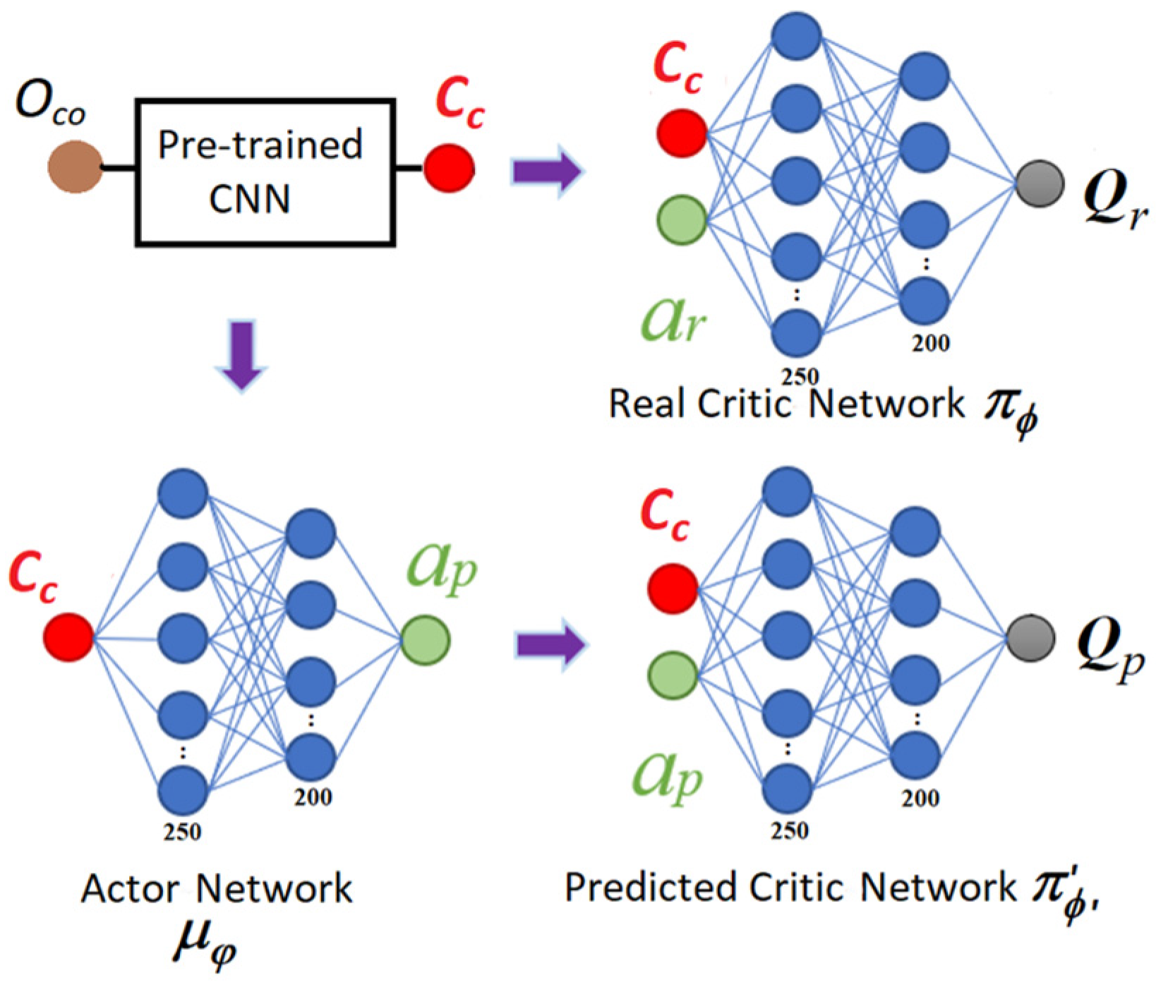
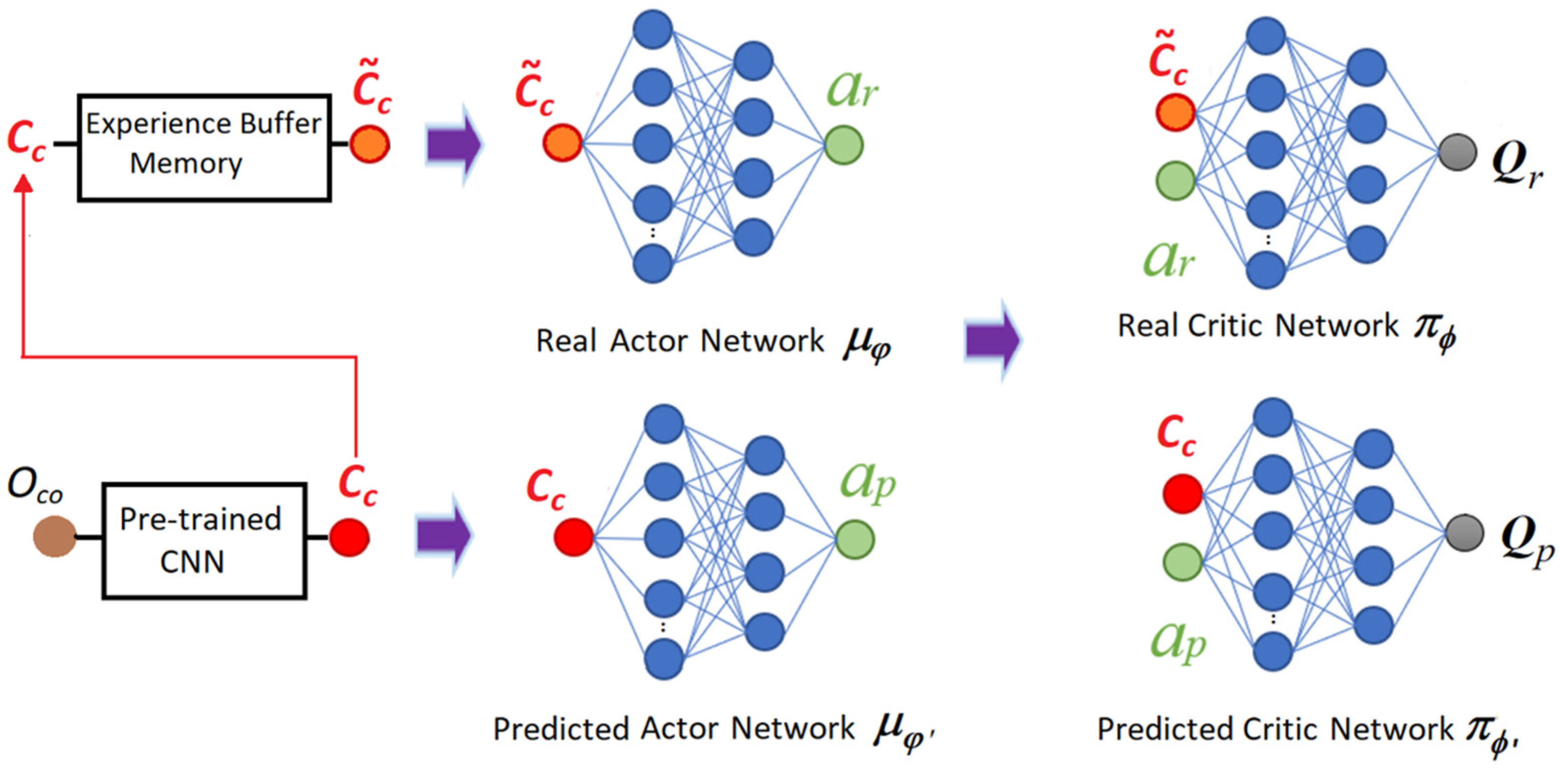
2.5. Deep Reinforcement Learning Phase

The network configuration in this phase remains aligned with the one introduced in the previous phase, as it is grounded in the same algorithm. This implementation retains the twin components from the previous phase, while incorporating the reward r, as defined in Equation (11).

$$r=\left\{\begin{array}{c}10 if the agent detects the target\\ -1 if the agent collides with a wall \\ -0.1 otherwise\end{array}\right.$$

(11)

Within the framework of DRL, one time step corresponds to a negative reward r (−0.1), in this manner, if the robotic agent takes more time to reach its objective, the loss value increases, punishing its movements. It is worth noting that an episode finishes only if the agent detects the target.

$${\mathcal{L}}_{critic}={\displaystyle \frac{1}{N}}\sum _{i=1}^N{\left(Q_p-\left(r+\gamma \times Q_r\right)\right)}^2$$

(12)

where $\gamma$ is the discount factor (0.9) and $r$ is the reward.

In the DRL phase, the predicted critic network is updated to decrease the critic loss function given by (12), and the predicted actor network is updated to decrease the actor loss function ${\mathcal{L}}_{actor}=-{\displaystyle \frac{1}{N}}\sum _{i=1}^N{Q}_p$. In both networks, the Adam optimizer is used to update the connection weights. The updated connection weights are transferred to the real critic network and real actor network using soft target methods (8) and (9), with smoothing factor $\tau$ equal to 0.1.

2.6. Characteristics of the Components Used

The components used are outlined in

Table 3. Components used in robotic agent.

Hardware	Technical Specifications
JETSON NANO NVIDIA, California, USA	GPU 128-core Maxwell CPU Quad-core ARM A57 a 1.43GHz 4Gb RAM 64bits
CAMERA Shenzhen City Wazney Electronic Technology Co., Futian District, China	Webcam HD 1080p USB Plug and Play
ULTRASONIC SENSOR Shenzhen Robotlinking Technology Co., Futian District, China	HC-SR04, Measuring range 2 cm to 400 cm, 5 v
MOTORS Shenzhen Jixin Micro Motor Co., Baoan District, China	3–50 v tension nominal, 14,425–23,000 rpm 0.11–0.486 A
SERVOMOTOR Yueqing Yidi Electronic Co., Zhejiang, China	Torque 2.5 kg/cm, 4.8–6 v, 32 × 32 × 12 mm
BATTERY Dongguan Wiliyoung Electronics Co., Guangdong Province, China	10,000 mA, Port de 5 v/2 A, 67.6 × 15.9 × 142.8 mm

. As indicated, a mobile GPU system with restricted capacity is employed for the implementation.

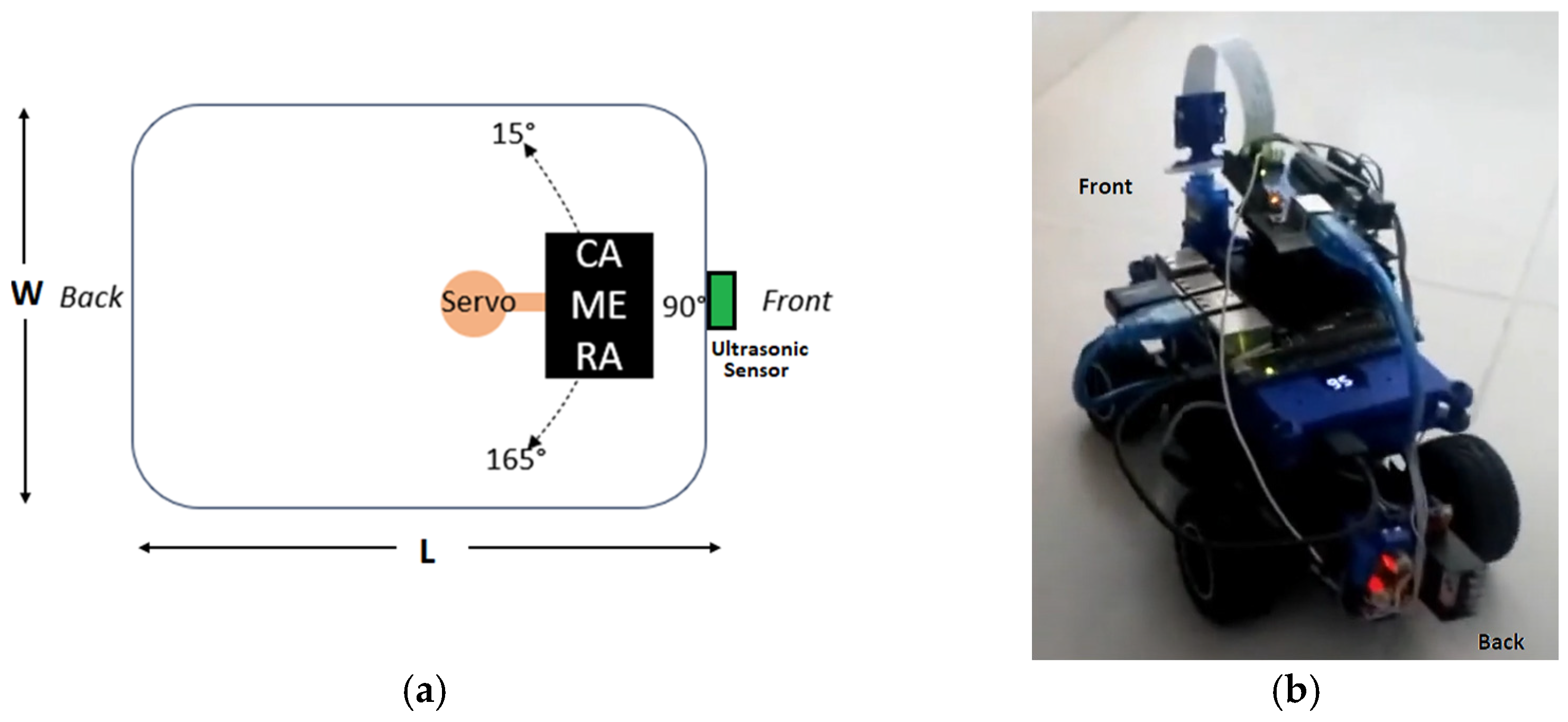
2.7. Robotic Agent Configuration

This section details the kinematic properties of a mobile robot, addressing its analysis through a kinematic model. It is considered an automobile-type robot (1, 1) that is characterized by having two distinct inputs: $u_1$, which represents the linear velocity of the fixed rear wheels, and $u_2$, which indicates the rotational speed of the steering wheels, as shown in Figure 6.

Figure 6 shows variables such as L, which corresponds to the length from axis to axis; the point P, which represents the origin of the moving reference axes; ${\theta }_0$, which is the angle of orientation of the moving reference frame; $V_p$, velocity at point P; ${\beta }_0$, the angle of orientation of the velocity of the point P; and the point Q, which represents the origin of the linear velocity $u_1$. Considering point Q, we obtain:

$$\dot{x_1}=u_1\mathit{cos}{\theta }_o$$

(13)

$$\dot{x_2}=u_1\mathit{sin}{\theta }_o$$

(14)

$$\dot{{\theta }_0}=u_2$$

(15)

The agent has two motors, one that controls the advance, $u_1$, and another that controls the direction of the front wheels, $u_2$. Equations (13)–(15) correspond to the kinematic model of the robotic agent and are used to obtain the values of angular and linear velocities, shown in Figure 6; these calculations are found in Appendix A. Velocities of the Agent.

3. Experiments

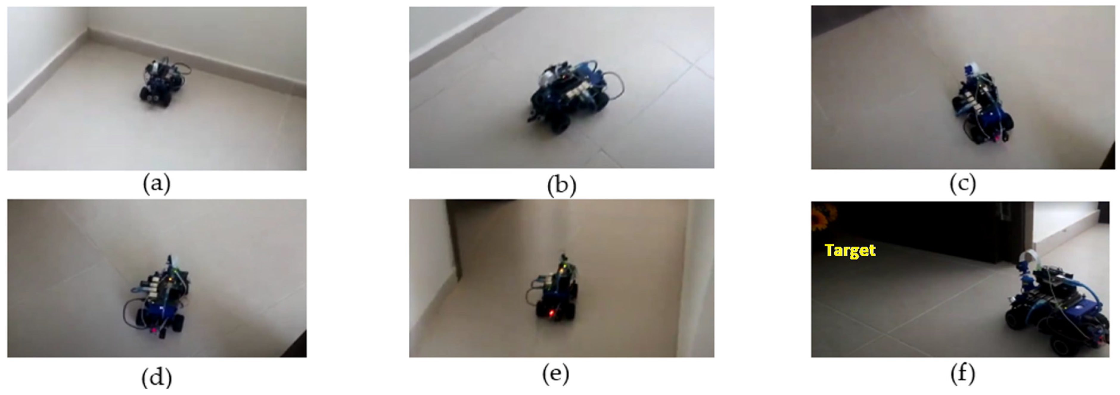
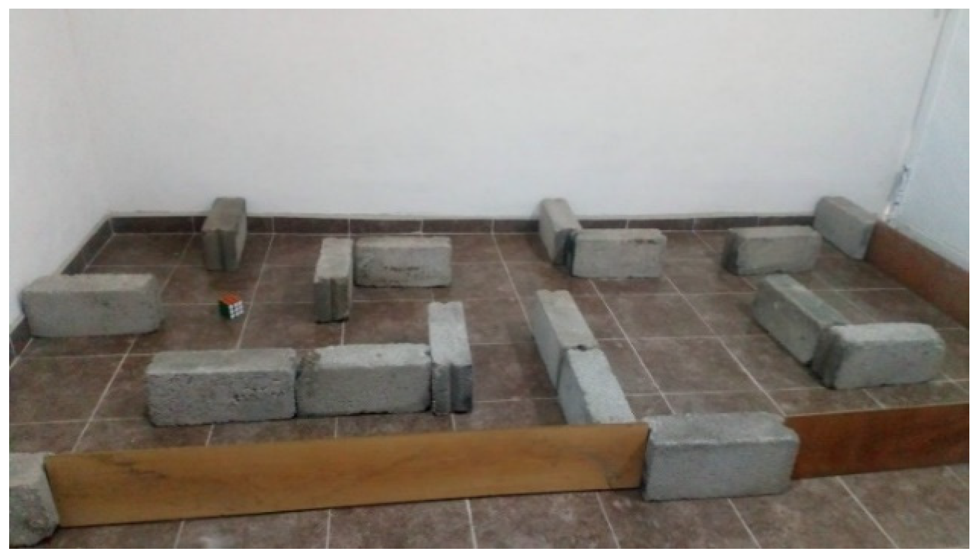
3.1. Static Environment

In the first phase of the experiment, the agent was tasked with locating an object within a static physical environment. To accomplish this, three distinct static environments were utilized, in which the initial position of the robot agent and the position of the target object were varied. Figure 7 shows three static environments, with an initial position of the robotic agent (black box) and a position of the target object (green box). As mentioned before, the positions of the agent and the target varied. In this experiment, the SSL, USL, and DRL phases were trained in environment (a), while environments (b) and (c) involved training and inference of the DRL phase.

The learning process started in the SSL phase. If the agent consistently achieved the upper threshold of learning level A for ten consecutive iterations (T = 10), it indicated the need for a more advanced learning system, the USL phase. The choice of 10 consecutive successful iterations as a threshold for transitioning between learning stages (from SSL to USL, and from USL to DRL) was based on empirical testing [24]. Through experimentation, we observed that, when the agent exhibited consistent navigation behavior, such as completing trajectories with minimal deviation or corrective oscillation, for at least 10 consecutive episodes, it indicated that the current internal representation or learning stage was sufficiently stable to advance. Similarly, if the agent maintained the highest level of learning for ten consecutive iterations during the USL phase, it suggested the application of the DRL phase. This sequential progression from SSL to DRL via USL is necessary when dealing with complex environments. By avoiding the direct implementation of DRL without the preceding SSL and USL phases, the agent minimizes the time and resources required to comprehend a complex environment effectively.

Figure 8 showcases the trajectory followed by the previously trained robotic agent through all learning phases using static environments (a)–(c), evaluated in (c) of Figure 7. The agent started from the initial position marked by a black box, which is position (a), and ultimately reached the location where a target object was found. The agent’s position in each time step from (a) to (f) corresponds to photograph numbers from (a) to (f) of Figure 8. In the initial position, (a), the agent selected the action “forward” from some possible actions {“forward”, “turn left”}, according to ultrasonic signals. This selected action provided the best quality based on the agent’s experience as reflected in the trained predicted actor network. Similarly, the agent selected “forward” in time step (b) and reached position (c). In this position, the agent found an obstacle to its front, so three pictures were taken. Because none of the three pictures presented the target object, the agent generated $O_{co}$, then trained CNN 2 interpreted that collision case $C_c$ is 3, meaning to [1, 1, 0]. Using its experience, the agent took the “right turn” as the best action, and then took the “forward” action to reach position (e). In position (e), the agent found an obstacle to its front, so three pictures were taken by the agent. In this case, CNN1 detected the target object in one of these three pictures (left side picture), and then the robotic agent took the “left turn” action and accomplished the mission in position (f).

The same set of hyperparameters was used across all three learning phases (SSL, USL, and DRL) to maintain consistency. These include a learning rate of 0.001, discount factor γ = 0.9, smoothing factor τ = 0.1, policy update delays every two iterations, batch size = 1, and replay buffer size of 10,000. The optimizer used was Adam. These values were empirically tuned for stable training under the computational constraints of the Jetson Nano. The full configuration files (software version 1.102.1) are available in the accompanying GitHub repository.

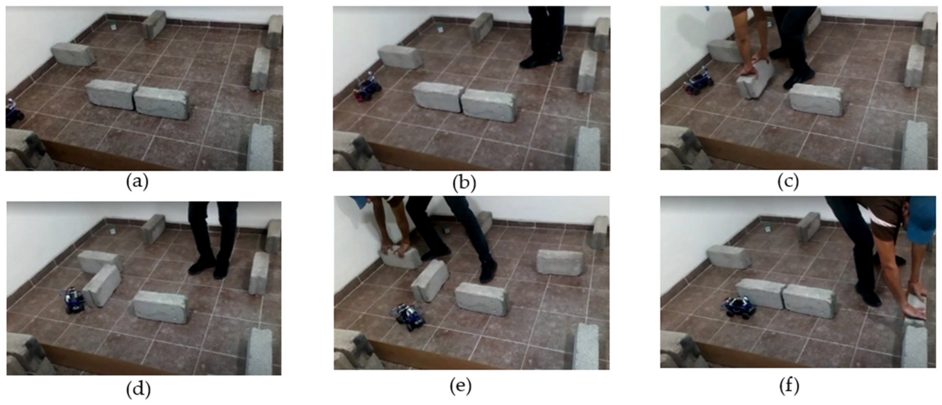
3.2. Dynamic Environment

In the second phase of the experiment, the main goal of the robotic agent was to locate a Rubik’s Cube within a dynamic environment, as depicted in Figure 9. This environment was characterized by the continuous movement and rearrangement of blocks, altering the environment perceived by the agent.

As shown in the videos presented as Supplementary Materials and in Figure 10, the robot agent avoided obstacles in all cases, even when the environment suddenly changed. However, training in such an environment is inherently time-consuming, due to the gradual depletion of the robot’s batteries, resulting in varying displacement lengths. In the dynamic environment, the experience accumulated by the agent itself was not helpful enough, so a large amount of experience buffer memory was required. Additionally, it was observed that the number of time steps needed to detect the target object varied depending on the decisions made by the actor network.

4. Results

We compared the performance of each learning phase in terms of “Experience Buffer Size”, “Computational Cost”, “Learning Oscillation”, and “Reaction Delay”, whose concepts will be explained later.

Table 4. Comparison of four different issues in three learning phases.

PHASE	Experience Buffer Size	Computational Cost	Learning Oscillation	Reaction Delay
SSL	50	10%	0.4127	0.1 s
USL	640	60%	0.0939	0.1 s
DRL	850	90%	0.0034	0.1 s

provides the comparison of results among the three learning phases.

The measurement methods of each one of the four concepts in Table 4, and how the values obtained were analyzed, are explained as follows.

• Experience Buffer Size was the amount of experience generated during each learning phase. In the NRNH-AR algorithm, for each time step after an action is selected, the experience performed is added into the experience buffer memory. This number is equivalent to the time steps required for the convergence of each learning phase.
• Computational Cost was measured as the average occupation percentage of the GPU of the Jetson Nano during each learning phase. For example, in the case of SSL, the average occupation is, on average, 10% of the full capacity of the Jetson Nano’s GPU. In contrast, in the DRL phase, on average, 90% of the total capacity must be used to solve the problem.
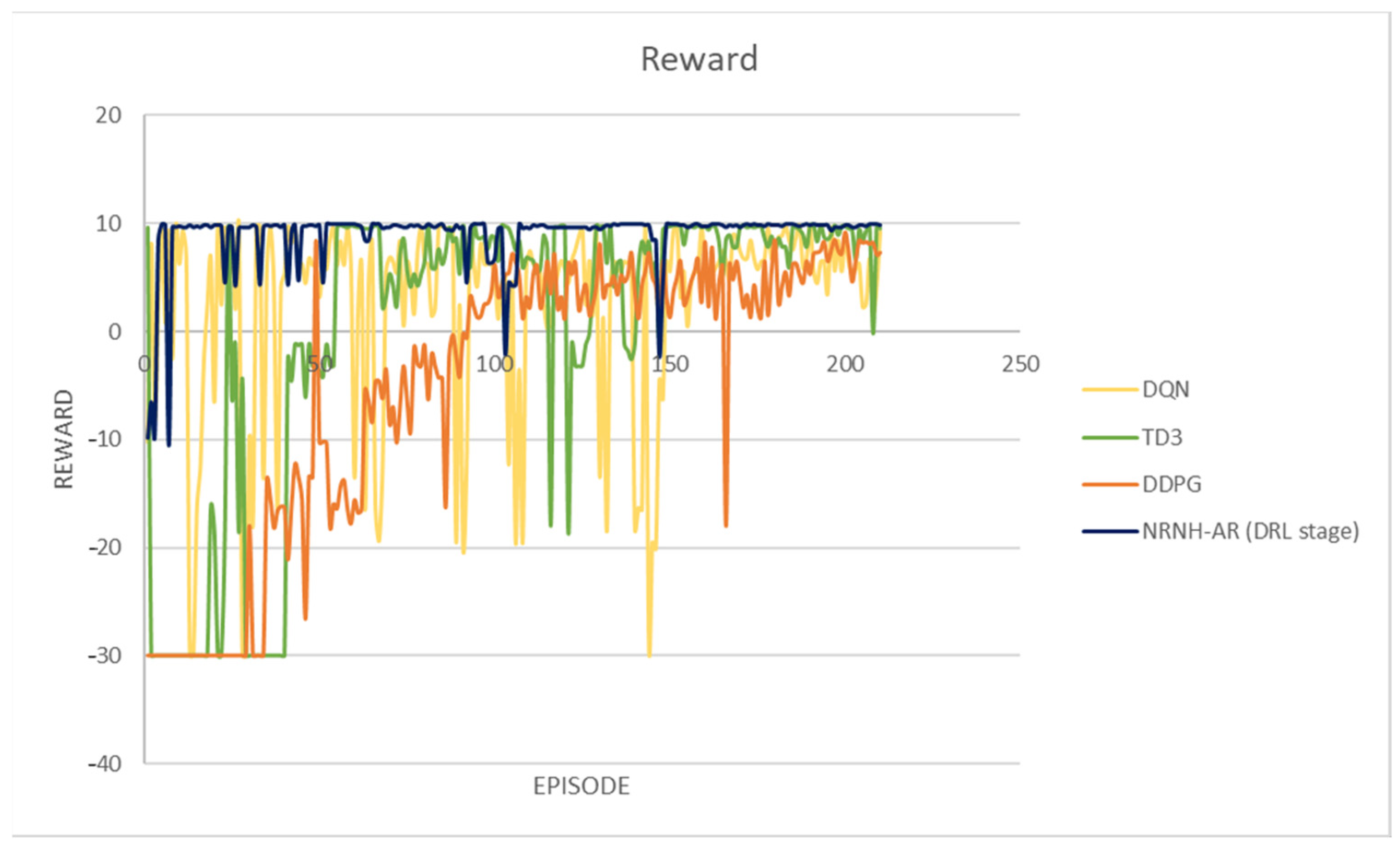
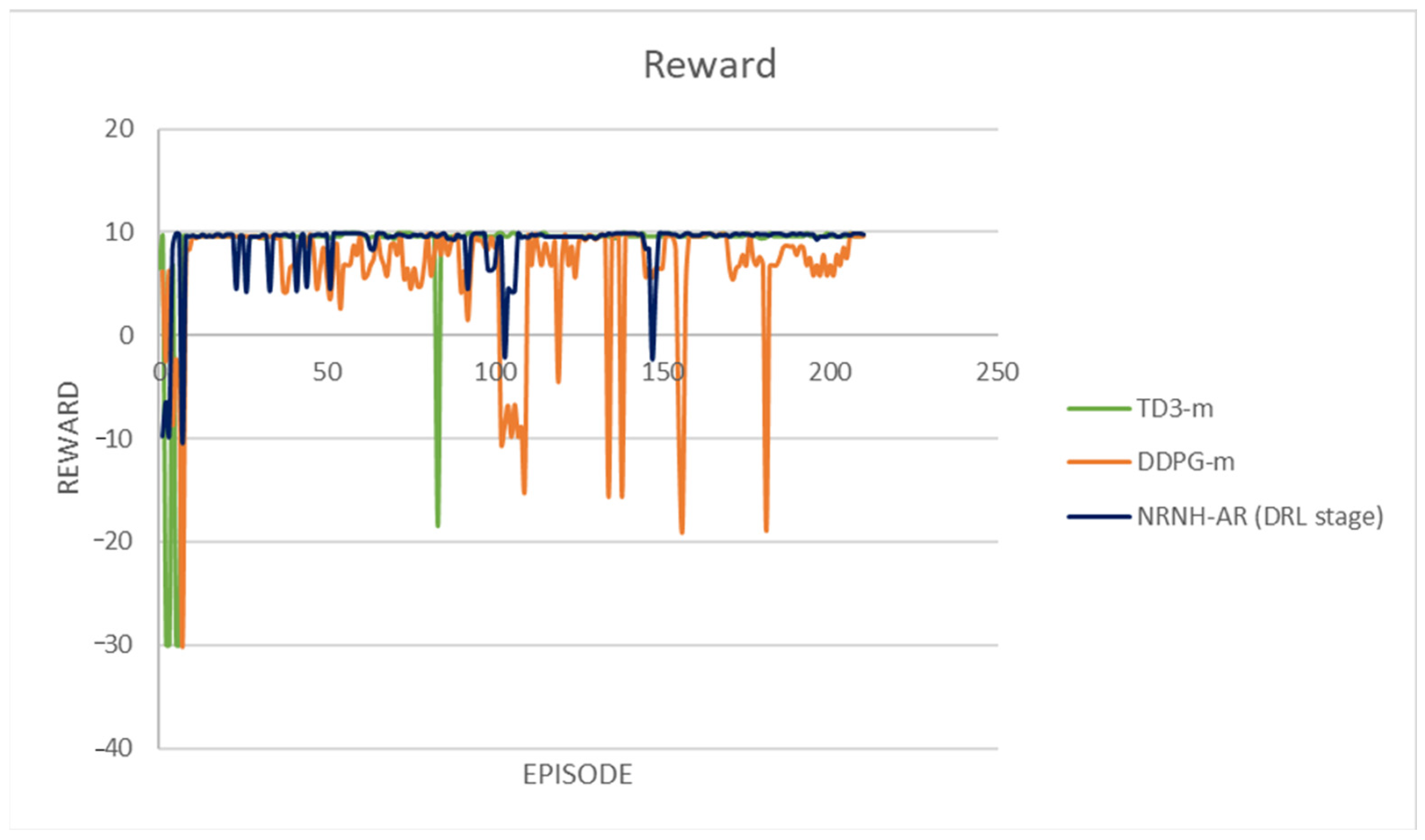
• Learning Oscillation was calculated as the standard deviation from the average learning level A in each phase. As expected, in the SSL phase, the robotic agent randomly selects an action to gain environmental information as quickly as possible, so the oscillation of the learning level is larger compared with the following two learning phases. The robotic agent acquires experience and evolves by updating the connection weights of the predicted actor network, learning is established, and oscillation is reduced. As mentioned before, the connection weights of the predicted actor network are updated to maximize the quality of the action performed.
• Reaction Delay was defined as the time elapsed from the robotic agent taking three images to performing a corresponding action. This value is essential in real applications because the total elapsed time from the start to detecting the target object is proportional to this value. From Table 4, the reaction delay is only 0.1 s in all learning phases, indicating a possible real-world application.

Static Environment

In a critical analysis of the scientific literature related to mobile robotics, a variety of algorithms implementing DRL can be observed, as shown in

Table 5. Methods of DRL in robotics in static environments.

Method	Hardware	Software	Obstacle Evasion	* Episodes	* Accuracy	Simulation	Physical Robot
GNND Multi-Robot [21]	3.2 GHz i7-8700 CPU and an Nvidia GTX 1080Ti GPU with 32	2D cluttered	Yes	3.0 × 104	99.50%	Yes	No
I3A [19]	Velodyne VLP-16	SemanticKitti	Yes	5.6 × 106	52.50%	Yes	No
FAM-HGNN [18]	2.2 GHz i7-10870 CPU Nvidia GeForce RTX 3060 GPU with 6 GB	OpenAI gym	Yes	1.0 × 107	96.00%	Yes	No
DQN algorithm [20]	Intel core i7 8GBRAM, Nvidia 940mx	ROS Gazebo	Yes	400	90.00%	Yes	No
DenseCAvoid [22]	Intel Xeon 3.6 GHz processor and an Nvidia GeForce RTX 2080Ti GPU	Gazebo 8.6	No	300	85.00%	Yes	No
DQN algorithm [9]	Raspberry Pi 3	ROS Gazebo	Yes	1500	60.00%	Yes	Yes
Ours	Jetson Nano 4GB 64bits	Python 3.12.5	Yes	210	97.62%	Yes	Yes

Note: * The Episodes and Accuracy of each method were reported by the authors in different environments using different targets.

. It is important to note that most of these algorithms are primarily limited to simulation environments and have not been extensively tested in physical robotics.

An exceptional case in Table 5 is the DQN-based algorithm proposed in [9], which has demonstrated its applicability in physical robotics under real-world environments. However, despite its real-world utility, the work of [9] has notable limitations in terms of efficiency. Specifically, this algorithm achieves an accuracy of only 60% after extensive training over 1500 epochs. In contrast, the proposed NRNH-AR algorithm surpasses this performance. With a considerably shorter training period of just 210 episodes, our algorithm achieves an accuracy of 97.62%. This superior accuracy demonstrates the robustness and superiority of NRNH-AR compared to the DQN-based algorithm. It is worth noting that the environments used for each method are different from each other.

Furthermore, it is important to highlight that existing research in the field of mobile robotics often relies on high-end hardware, as depicted in Table 5. While this may enhance the effectiveness of simulations, its practical feasibility in mobile robotics with limited resources is questionable. Therefore, it is crucial to continue developing and optimizing algorithms like NRNH-AR, that not only exhibit superior performance, but are also practical and viable for implementation in mobile robotics.

Table 5 presents a consolidated comparison of selected DRL-based methods in mobile robotics to complement the narrative review provided in the Introduction. While similar points are discussed earlier, this table allows for clearer quantitative comparison across hardware and training configurations.

Figure 11 illustrates the episode-wise rewards obtained by the standard deep reinforcement learning algorithms, DQN (yellow), TD3 (green), and DDPG (orange), compared to the DRL stage of the proposed NRNH-AR model (navy blue) across 210 training episodes in the environment shown in Figure 7a. It can be clearly observed that the NRNH-AR agent reaches high and stable reward values from the very beginning of the training process. This rapid convergence can be attributed to the previous self-supervised and unsupervised learning stages that provided the agent with structured, informative representations before reinforcement learning began.

In contrast, the baseline algorithms (DQN, TD3, DDPG) exhibit highly unstable learning dynamics in early episodes, with frequent oscillations and negative rewards. DDPG struggles significantly during the first 100 episodes, suggesting poor initial policy exploration. Although all three baseline algorithms eventually stabilize and improve their performance, they require substantially more episodes to reach comparable performance levels to NRNH-AR.

Figure 12 presents the performance of three reinforcement learning algorithms, TD3-m, DDPG-m, and NRNH-AR, which was trained in the environment shown in Figure 7a, after integrating SSL and USL as pre-training stages before DRL. This pre-training strategy was designed to improve sample efficiency and reduce the overall training time, enabling the agent to extract structural knowledge from the environment before reward-driven interaction began. It is worth mentioning that the DQN is not included in this evaluation, because it uses only two networks, whose structures are not compatible with the SSL and USL phases.

The impact of the SSL and USL phases is evident when comparing the behaviors of TD3-m and DDPG-m with their original versions, as shown in Figure 11. TD3-m and DDPG-m exhibit significantly smoother learning trajectories from the beginning of training, avoiding the prolonged periods of instability seen earlier. Overall, the results reinforce the importance of tri-fold learning, e.g., SSL and USL before applying DRL. The good performance of TD3-m indicates that the replacement of our DRL with TD3-m or other more efficient DRLs compatible with previous SSL and USL phases can be useful.

Table 6. Accuracy comparison of DRL algorithms and the proposed NRNH-AR method in the physical robot environment.

	DQN	DDPG	TD3	OUR	DDPG-m	TD3-m
Accuracy	81.90%	56.19%	68.57%	97.62%	86.19%	96.19

shows that the proposed NRNH-AR method achieves the highest accuracy (97.62%) among all tested DRL algorithms in the physical robot environment. Compared to the standard versions of DQN (81.90%), DDPG (56.19%), and TD3 (68.57%), NRNH-AR outperforms them significantly, indicating better policy learning and generalization under real-world conditions.

Moreover, the modified versions DDPG-m and TD3-m, which were adapted for low-resource hardware and tuned to the test environment, achieve improved results (86.19% and 96.19%, respectively) over their original counterparts. However, even the best-performing baseline (TD3-m) remains slightly below the proposed method.

In dynamic environments, the proposed NRNH-AR algorithm achieved an accuracy of 86%. Baseline algorithms were not evaluated under dynamic conditions, as their low performance in static environments did not justify further testing. Additionally, comparing against modified versions (DDPG-m and TD3-m) would not be appropriate, since they incorporate the same pre-training methodology as NRNH-AR and do not represent the original algorithms.

Based on our observations, the performance of NRNH-AR exhibits diminishing returns beyond a certain amount of training data. For example, CNN 2 achieves adequate generalization when trained with approximately 623 samples, as indicated by a loss value under 1.0. Similarly, learning oscillation in the SSL and USL phases stabilizes after around 200–250 episodes. These empirical thresholds allow us to keep training time and memory usage low, in line with our focus on constrained hardware.

In the dynamic scenarios, the configuration of the environment was manually modified during navigation by repositioning obstacle blocks. These operator-controlled changes allowed for reproducible yet dynamic conditions, simulating the presence of moving elements or restructured paths in real-world environments.

5. Conclusions

In this paper, we introduced the NRNH-AR algorithm for small-scale physical robotics; although this study targets small mobile robots, the modular structure of NRNH-AR allows adaptation to larger robotic platforms. Our algorithm, designed with a tri-fold learning approach (SSL, USL, and DRL), optimizes the use of computational and memory resources, critical aspects in energy-efficient robotics. This tri-fold design shows high adaptability to static and dynamic environments, with effectiveness levels of 97.62% and 86.0%, respectively, in our trials.

This work confirms that combining SSL and USL with DRL in a three-stage learning pipeline can enhance reinforcement learning performance. The NRNH-AR model, which integrates these stages, outperforms baseline DRL algorithms, such as DQN, DDPG, and TD3, in both learning speed and final policy quality. The comparison between raw DRL approaches and their pre-trained counterparts illustrates that proper representation learning can reduce the need for prolonged exploration, leading to more sample-efficient and stable learning.

With low computational cost, NRNH-AR proves to be a viable solution for implementation in small-scale physical robotic agents. However, ongoing research and optimization efforts are crucial to maximizing its effectiveness and efficiency in practical applications. The obtained findings demonstrate the effectiveness of hybrid learning systems that leverage unlabeled data before applying reinforcement learning, especially in real-world scenarios where data collection and interaction with the environment are costly or constrained.

The principal limitation in the operation of physical robotic agents is their short battery life, a common problem for all navigation robots using batteries. In our robotic agent, we used a battery whose life was approximately 1 h. The battery life is a critical factor, as the displacement of the robotic agent varies depending on the battery charge level, regardless of the ability to control the rotational speed. The operating range of module L298N is 3–5 V, with a power output of 0.51 W. This variability in the power supply necessitates adjustments in the networks, even if they have already achieved optimal weights, as they adapt to the battery load in use. This problem suggests several future research directions, including the exploration of alternative network architectures and optimization techniques to improve computational efficiency and reduce training time. Additionally, NRNH-AR will also be compared with lightweight algorithms designed explicitly for small physical robots under similar real-world conditions, in order to further validate its performance in hardware-constrained scenarios. Although our comparison includes popular DRL algorithms (DQN, DDPG, TD3), future research should aim to benchmark NRNH-AR against lightweight DRL or hybrid methods specifically optimized for mobile robotics and tested on real robots with constrained hardware. This would further validate its competitiveness and practical relevance in the field.

References

1. Wen, T.; Wang, X.; Zheng, Z.; Sun, Z. A DRL-based Path Planning Method for Wheeled Mobile Robots in Unknown Environments. Comput. Electr. Eng. 2024, 118, 109425. [Google Scholar] [CrossRef]
2. Bar, N.F.; Karakose, M. Collaborative Approach for Swarm Robot Systems Based on Distributed DRL. Eng. Sci. Technol. Int. J. 2024, 53, 101701. [Google Scholar] [CrossRef]
3. Tang, W.; Wu, F.; Lin, S.-W.; Ding, Z.; Liu, J.; Liu, Y.; He, J. Causal Deconfounding Deep Reinforcement Learning for Mobile Robot Motion Planning. Knowl.-Based Syst. 2024, 303, 112406. [Google Scholar] [CrossRef]
4. Cui, T.; Yang, Y.; Jia, F.; Jin, J.; Ye, Y.; Bai, R. Mobile Robot Sequential Decision Making using a Deep Reinforcement Learning Hyper-heuristic Approach. Expert Syst. Appl. 2024, 257, 124959. [Google Scholar] [CrossRef]
5. Kim, D.; Carballo, D.; Di Carlo, J.; Katz, B.; Bledt, G.; Lim, B.; Kim, S. Vision aided Dynamic Exploration of Unstructed Terrain with Small-Scale Quadruped Robot. In Proceedings of the 2020 IEEE International Conference on Robotics and Automation (ICRA), Paris, France, 31 May–31 Agust 2020. [Google Scholar] [CrossRef]
6. Bayati, M.; Fotouhi, R. A Mobile Robotic Platform for Crop Monitoring. Adv. Robot. Autom. 2018, 7, 186. [Google Scholar] [CrossRef]
7. Yoosuf, L.; Gafoor, A.; Nizam, Y. Designing and Testing a Robot for Removing Sharp Metal Objects from Roads. AIP Conf. Proc. 2024, 3245, 020004. [Google Scholar] [CrossRef]
8. Ge, L.; Fang, Z.; Li, H.; Zhang, L.; Zeng, W.; Xiao, X. Study of a Small Robot for Mine Hole Detection. Appl. Sci. 2023, 13, 13249. [Google Scholar] [CrossRef]
9. Balachandram, A.; Lal, S.A.; Sreedharan, P. Autonomous Navigation of an AMR using Deep Reinforcement Learning in a Warehouse Environment. In Proceedings of the IEEE 2nd Mysore Sub Section International Conference (MysuruCon), Mysuru, India, 16–17 October 2022. [Google Scholar] [CrossRef]
10. Ozdemir, K.; Tuncer, A. Navigation of Autonomous Mobile Robots in Dynamic Unknown Environments Based on Dueling Double Deep Q Networks. Eng. Appl. Artif. Intell. 2024, 139, 109498. [Google Scholar] [CrossRef]
11. Zhang, B.; Li, G.; Zhang, J.; Bai, X. A Reliable Traversability Learning Method Based on Human-Demonstrated Risk Cost Mapping for Mobile Robots over Uneven Terrain. Eng. Appl. Artif. Intell. 2024, 138, 109339. [Google Scholar] [CrossRef]
12. Li, P.; Chen, D.; Wang, Y.; Zhang, L.; Zhao, S. Path Planning of Mobile Robot Based on Improved TD3 Algorithm in Dynamic Environment. Heliyon 2024, 10, e32167. [Google Scholar] [CrossRef] [PubMed]
13. Li, Z.; Shi, N.; Zhao, L.; Zhang, M. Deep Reinforcement Learning Path Planning and Task Allocation for Multi-Robot Collaboration. Alex. Eng. J. 2024, 109, 418–423. [Google Scholar] [CrossRef]
14. Cheng, B.; Xie, T.; Wang, L.; Tan, Q.; Cao, X. Deep Reinforcement Learning Driven Cost Minimization for Batch Order Scheduling in Robotic Mobile Fulfillment Systems. Expert Syst. Appl. 2024, 255, 124589. [Google Scholar] [CrossRef]
15. Xiao, H.; Chen, C.; Zhang, G.; Chen, C.L.P. Reinforcement Learning-Driven Dynamic Obstacle Avoidance for Mobile Robot Trajectory Tracking. Knowl.-Based Syst. 2024, 297, 111974. [Google Scholar] [CrossRef]
16. Sun, H.; Zhang, C.; Hu, C.; Zhang, J. Event-Triggered Reconfigurable Reinforcement Learning Motion-Planning Approach for Mobile Robot in Unknown Dynamic Environments. Eng. Appl. Artif. Intell. 2023, 123, 106197. [Google Scholar] [CrossRef]
17. Deshpande, S.V.; Ra, H.; Ibrahim, B.S.K.K.; Ponnuru, M.D.S. Mobile Robot Path Planning using Deep Deterministic Policy Gradient with Differential Gaming (DDPG-DG) Exploration. Cogn. Robot. 2024, 4, 156–173. [Google Scholar] [CrossRef]
18. Zhang, F.; Xuan, C.; Lam, H.-K. An Obstacle Avoidance-Specific Reinforcement Learning Method Based on Fuzzy Attention Mechanism and Heterogeneous Graph Neural Networks. Eng. Appl. Artif. Intell. 2024, 130, 107764. [Google Scholar] [CrossRef]
19. Alonso, L.; Riazuelo, L.; Montesana, L.; Murillo, A.C. Domain Adaptation in LiDAR Semantic Segmentation by Aligning Class Distributions. In Proceedings of the International Conference on Informatics in Control, Automation and Robotics (ICINCO), Virtual, 6–8 July 2020. [Google Scholar] [CrossRef]
20. Escobar-Naranjo, J.; Caiza, G.; Ayala, P.; Jordan, E.; Garcia, C.A.; Garcia, M.V. Autonomous Navigation of Robots: Optimization with DQN. Appl. Sci. 2023, 13, 7202. [Google Scholar] [CrossRef]
21. Sun, X.; Zhang, Q.; Wei, Y.; Liu, M. Risk-Aware Deep Reinforcement Learning for Robot Crowd Navigation. Electronics 2023, 12, 4744. [Google Scholar] [CrossRef]
22. Sathyamoorthy, A.J.; Liang, J.; Patel, U.; Guan, T.; Chandra, R.; Manocha, D. DenseCAvoid: Real-time Navigation in Dense Crowds using Anticipatory Behaviors. In Proceedings of the IEEE International Conference on Robotics and Automation (ICRA), Paris, France, 31 May–31 August 2020. [Google Scholar] [CrossRef]
23. Tang, Y.C.; Qi, S.J.; Zhu, L.X.; Zhuo, X.R.; Zhang, Y.Q.; Meng, F. Obstacle Avoidance Motion in Mobile Robotics. J. Syst. Simul. 2024, 36, 1–26. [Google Scholar] [CrossRef]
24. Vasquez, C.; Nakano, M.; Velasco, M. Practical Application of Deep Reinforcement Learning in Physical Robotics. In Proceedings of the 3rd International Conference on Intelligent Software Methodologies, Tools, and Techniques (SOMET 2024), Cancun, Mexico, 24–26 September 2024. [Google Scholar] [CrossRef]
25. Howard, A.; Sandler, M.; Chen, B.; Wang, W.; Chen, L.-C.; Tan, M.; Chu, G.; Vasudevan, V.; Zhu, Y.; Pang, R.; et al. Searching for MobileNetV3. In Proceedings of the IEEE/CVF International Conference on Computer Vision (ICCV), Seoul, Republic of Korea, 27 October–2 November 2019. [Google Scholar] [CrossRef]
Figure 1. General diagram of NRNH-AR algorithm.
Applsci 15 08149 g001
Figure 2. (a) Camera and ultrasonic sensor on the robotic agent. The camera is positioned by a servomotor at 15°, 90°, and 165°. (b) The robotic agent has dimensions of 235 mm (L) × 132 mm (W) × 180 mm (H), and 840 g.
Applsci 15 08149 g002
Figure 3. CNN training process.
Applsci 15 08149 g003
Figure 4. Network structures in the SSL phase.
Applsci 15 08149 g004
Figure 5. Network structures in the USL phase.
Applsci 15 08149 g005
Figure 6. Free body diagram of the mobile robot (1, 1).
Applsci 15 08149 g006
Figure 7. Configuration of three physical static environments (ac) used for evaluation.
Applsci 15 08149 g007
Figure 8. The process of moving the agent in a static environment. (a) Starting position, (b) after “forward” action, (c) stopped due to an obstacle in front of the agent, (d) after “right turn” action, (e) “forward” action selected, and (f) the target object is detected. For a better understanding, please see https://www.youtube.com/watch?v=SUtYk2Ee1DU accessed on 18 March 2022.
Applsci 15 08149 g008
Figure 9. The environment where the NRNHN-AR algorithm was tested.
Applsci 15 08149 g009
Figure 10. Dynamic environment. (a) Starting position, (b) “forward” action is selected, (c) “turn right” action is selected and environment is modified, (d) environment is modified and “turn right” action is selected, (e) “forward” action is selected, (f) “turn left” action is selected and environment is modified. For a better understanding of the detailed movement of the agent, please see https://www.youtube.com/watch?v=SUtYk2Ee1DU accessed on 18 March 2022.
Applsci 15 08149 g010
Figure 11. Episode-wise reward comparison of DQN, TD3, DDPG, and NRNH-AR (DRL stage). The maximum number of steps per episode is 30.
Applsci 15 08149 g011
Figure 12. Reward after integrating SSL and USL pre-training into DRL algorithms. The maximum number of steps per episode is 30.
Applsci 15 08149 g012