Article

A Probability Integral Parameter Inversion Method Integrating a Selection-Weighted Iterative Robust Genetic Algorithm

1
School of Environment and Surveying Engineering, Suzhou University, Suzhou 234000, China
2
Coal Industry Engineering Research Center of Mining Area Environmental and Disaster Cooperative Monitoring, Anhui University of Science and Technology, Huainan 232001, China
3
Key Laboratory of Aviation-Aerospace-Ground Cooperative Monitoring and Early Warning of Coal Mining-Induced Disasters of Anhui Higher Education Institutes, Anhui University of Science and Technology, Huainan 232001, China
*
Authors to whom correspondence should be addressed.
Appl. Sci. 2025, 15(14), 8102; https://doi.org/10.3390/app15148102
Submission received: 22 May 2025 / Revised: 10 July 2025 / Accepted: 20 July 2025 / Published: 21 July 2025

Abstract

The accurate inversion of mining subsidence prediction parameters is key to the precise prediction of deformation during mining. However, the use of traditional genetic algorithms (GA) for inversion prediction has problems such as poor resistance to differences, and the accuracy of inversion parameters is affected when key monitoring points are missing. In response to these issues, a probability integral parameter inversion method is proposed in this study that integrates a selection-weighted iterative robust genetic algorithm. This method combines the selection-weighted iteration method with a genetic algorithm to determine the weights of different observation values, and then a probability integral parameter inversion method is constructed for the fusion selection-weighted iterative robust GA. The results indicate that the fusion selection-weighted iterative robust GA is stronger than the traditional GA, and the parameters obtained have higher accuracy and greater reliability. An experiment using real working face engineering showed that, compared with the GA method, the RMSE (root mean square error) of the proposed method is reduced by 24.4 mm and 37.5 mm, thus verifying the usability of this method.

1. Introduction

Coal resource mining operations cause surface damage such as movement and deformation of the Earth’s surface. When coal mining operations reach a certain stage, the surface facilities located within the deformation area can undergo deformation or damage [1,2,3,4,5]. Therefore, conducting research on mine deformation monitoring is extremely important for the restoration of the ecological environment and the control of subsidence disasters. The probability integration method (PIM) is a geometry-based mining subsidence prediction approach widely applied in China [6,7,8,9,10]. Parameter inversion usually involves the use of deformation data combined with the PIM to invert the mining subsidence prediction parameters. The accurate inversion of these parameters is a key prerequisite for the precise prediction of subsidence deformation. On the one hand, there are inevitably errors in surface measurement data; on the other, the inversion of probability integration parameters using surface measurement data is affected by the model errors of the probability integration method itself, resulting in poor stability and reliability. Therefore, further research of current parameter inversion methods is still needed.
Research shows that there are two types of methods commonly used in parameter prediction. The first is a parameter prediction method based on artificial intelligence (AI) [11,12,13,14,15,16,17], which uses a large number of measured prediction parameters and coal mining parameters as the training sets, and the parameters of the PIM are obtained through various artificial intelligence prediction models. The second method obtains probability integral parameters based on intelligent optimization algorithms [18,19,20,21,22,23,24,25,26,27,28,29]. This method first uses the PIM to establish the error equation between the cost function and the parameters of the PIM. Then, an intelligent optimization algorithm is used to perform the optimal estimation of the PIM parameters, thereby obtaining the optimal estimation value of the mining subsidence prediction parameters. It is difficult to achieve the optimal prediction of all PIM parameters using the AI-based method due to limitations in AI development and the complexity of mining subsidence problems. The PIM-based parameter acquisition method based on intelligent optimization algorithms can estimate all parameters optimally, but different intelligent optimization algorithms have different advantages and disadvantages. For example, the selection of initial parameters has a significant impact on the vector model method, and unfavorable initial values may fall into local optimal traps. GAs are susceptible to observation errors, which can inaccurately estimate PIM parameters. The above analysis shows that, between the two types of mining subsidence parameter inversion methods, the PIM parameter acquisition method based on intelligent optimization algorithms has certain advantages, but the selection of initial parameter values and the impact of observation value errors require further research.
Following an analysis of the literature, a PIM parameter inversion method is proposed in this study that integrates the selection-weighted iterative robust genetic algorithm (the weight matrix of different observations is updated by the IGG (Institute of Geodesy and Geophysics) weight function and the residuals of the observations, and the weights of the observations containing the error are reduced to achieve immunity). The method is as follows: first, based on the basic principle of obtaining PIM parameters based on an intelligent optimization algorithm, the error equation of the parameters is established. Second, the IGG weighting iteration function (the weight function of a robust estimation method) method is used [30,31,32], and a parameter cost equation based on the IGG method is constructed (increasing the influence of observation error on the parameter estimation accuracy). Finally, the parameter error equation is solved using the constructed parameter cost equation based on the IGG method to obtain the optimal PIM parameter value. The reliability and feasibility of the proposed method are proven using simulation experiments and specific engineering examples. Based on the simulation experiments, the influence of k value selection in the IGG method’s weight iteration function and the different survey line layout forms on the inversion probability integral parameters is discussed in detail. Finally, the conclusion of the study is presented.

2. Methods

2.1. The PIM Prediction Model

Chinese researchers of mining subsidence have developed the PIM, which is widely used in Chinese mines. According to the PIM prediction equation [18,19,20], the subsidence of the Earth’s surface at the mining working face can be expressed using Equation (1) to Equation (4):
W ( x , y ) = W m a x 0 D 3 1 r e π ( x s ) 2 r 2 d s 0 D 1 1 r e π ( y t ) 2 r 2 d t = W ( x ) W ( y ) W m a x
W m a x = m q c o s ( a )
W ( x ) = W m a x 2 e r f π t a n β H x + 1 e r f π t a n β H ( x L 3 ) + 1
W ( y ) = W m a x 2 e r f π t a n β H y + 1 e r f π t a n β H ( y L 1 ) + 1
In the equations, Wmax is the coal mining working face that causes the maximum subsidence of the Earth’s surface; m represents the thickness of the coal seam being mined; q is the subsidence coefficient; α is the inclination angle of the coal seam; (x,y) is the coordinates at any point on the surface; H is the average mining depth of the working surface; tanβ is the main influence tangent; L3 = D3S3S4, L1 = (D1S1S2) × sin(θ + α)/sinθ; θ is the greatest subsidence angle; D1 is the length of inclination of the working face; D3 is the length of the strike of the working face; S1, S2, S3, and S4 are the upper, lower, left, and right inflection point offsets of the working face, respectively; and r = H/tanβ is the main impact radius. Among these parameters, B = [q,tan β,θ,S1,S2,S3,S4] is the estimated parameter for subsidence using the probability integration method, and G = [m,H,x,y,α,D3,D1] is the geological parameter.

2.2. Construction and Solution of Conditional Equations

According to the mining subsidence and subsidence prediction model, the working face of the coal mine causes point A(x,y) on the Earth’s surface to sink, as shown in Equation (5):
W ( x , y ) = F ( B , G )
The relationship between subsidence and parameter P is established through Equation (5), and the error equation is as shown in Equation (6):
v j = W r j W p j
In the equation, W r j represents the measured subsidence value; and W p j represents the predicted subsidence value, where B is estimated (B = [q,tan β,θ,S1,S2,S3,S4]).
For Equation (6), when the number of measured subsidence values j ≥ 7, it can be linearized, and then the least squares method can be used to solve the linear equation. However, due to the highly nonlinear function of condition Equation (6), it is difficult to accurately solve the conventional measurement adjustment. Therefore, in order to obtain accurate subsidence prediction parameters using the probability integration method, an approach to solve Equation (6) is proposed in Section 2.3.

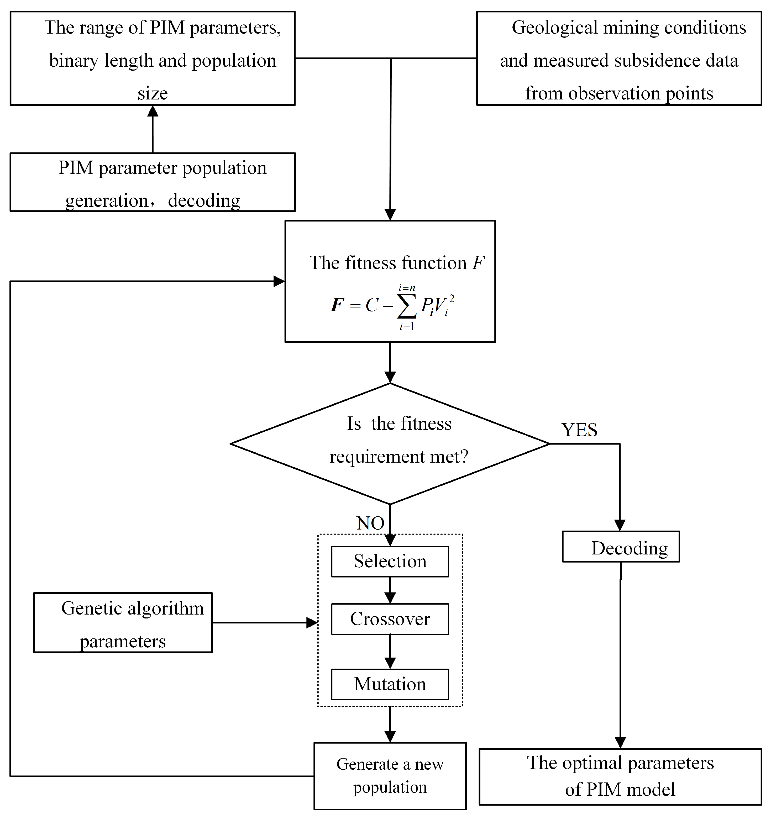
2.3. Prediction Parameters of PIM Solution Based on Robust Genetic Algorithm

Robust estimation is a parameter estimation method used in statistics. The stability of the method’s estimation results is maintained when there are outliers in the data or slight deviations in the model assumptions. This study adopts the robust estimation method—the selection-weighted iteration method—and combines it with a genetic algorithm to invert the parameters. The process is as follows: firstly, the weights of all measured subsidence values are equal, parameter inversion is performed using the genetic algorithm, and the predicted subsidence values of all points are calculated; secondly, the absolute residual value of each point is compared; finally, the selection-weighted iteration method is used to assign corresponding updated weights to each observation value, thereby adding the influence of the updated weights to the original square sum of residuals. Equation (7) is used for the minimum residual sum of squares after adding weights:
V m i n = i = 1 j P i v i 2
In Equation (7), Vmin is the minimum residual sum of squares after adding weights; Pi represents the weight corresponding to the observation value with the observation number i; j represents the number of points; and vi represents the absolute residual value between the i-th estimated subsidence and the actual subsidence.
This study adopts the IGG selection weighting iteration method [30,31,32], and the method for determining the weighting function using the IGG selection weighting iteration method is Equation (8):
P i = 1      v i 1.5 σ 1 v i + k      1.5 σ < v i 2.5 σ 0           v i > 2.5 σ
In Equation (8), k is a constant coefficient; σ is the mean square error of the observation value; and vi is the residual value of the i-th observation value fitting.
According to Equation (8), when |vi| is less than 1.5σ, the error contained in the corresponding observation value should be accidental. When |vi| is greater than 2.5σ, the corresponding observation value should contain a gross error (observational errors or data errors that deviate from normal values). When |vi| is greater than 1.5σ and less than or equal to 2.5σ, the corresponding observation value should contain a certain proportion of gross errors, and appropriate weights can be assigned to avoid being affected by gross errors.
This section describes a method for solving parameters based on a selection-weighted iterative robust GA. The method is carried out using the following six steps:
(1) When applying this method to solve the parameters based on the selection-weighted iterative robust genetic algorithm, the mining working face condition parameters G and the measured subsidence data are inputted. The interval position of parameter B is determined based on the mining working face condition parameters of adjacent working faces, and the parameters of the genetic algorithm are set (in this experiment, the number of iterations was maxGEN = 500, population size was NIND = 100, mutation rate was PM = 0.02, crossover rate was GGAP = 0.95, and binary encoding length was PRECI = 10).
(2) Population encoding and generation are carried out. According to the known parameters of the mine working face, the predicted subsidence parameter B in this mining area is within the known range; the binary encoding of each parameter is randomly generated using binary encoding rules to establish an initial population.
(3) The population binary code is decoded into parameter B, and the F of each individual in the population is solved by substituting parameter B for the probability integral model. The fitness calculation equation is as follows:
F = C V m i n
In the equation, C is a constant that makes F greater than zero.
(4) The ratio of individual fitness to overall fitness is calculated, which is the probability of the selected individual.
(5) Selection, crossover, and mutation operations are performed on populations and a new population is created. This can help determine the global and local search capabilities of the genetic algorithms.
(6) Iteration and termination are conducted. Steps (2)~(6) are repeated until the number of iterations or fitness meet the requirements, and then the iteration process is terminated. Finally, the binary encoding can be decoded to obtain accurate parameters for estimation.
The process outlined in Section 2.2 is presented in Figure 1 as a flowchart for solving parameters using the fusion selection-weighted iterative robust GA.

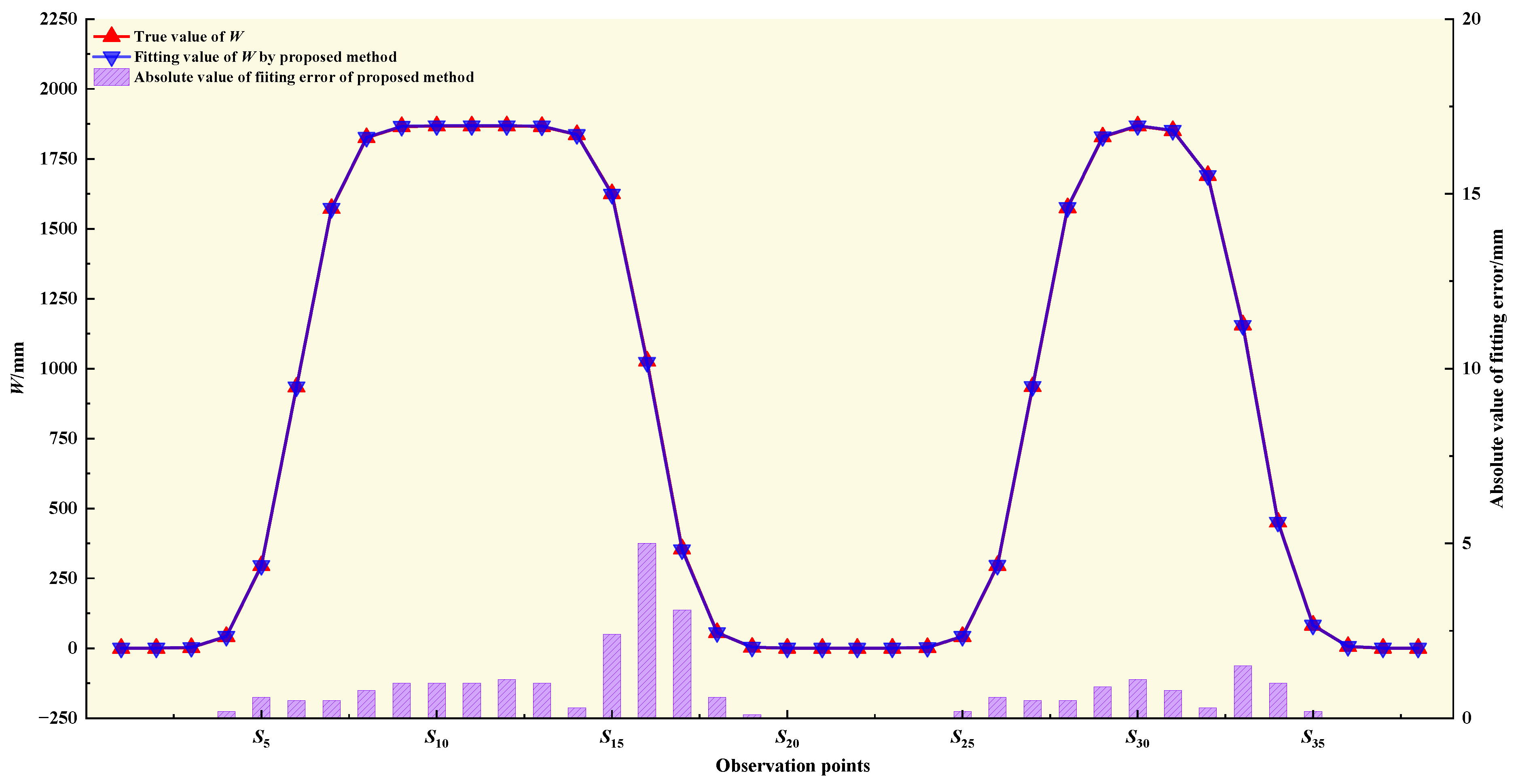
3. Simulated Experiment

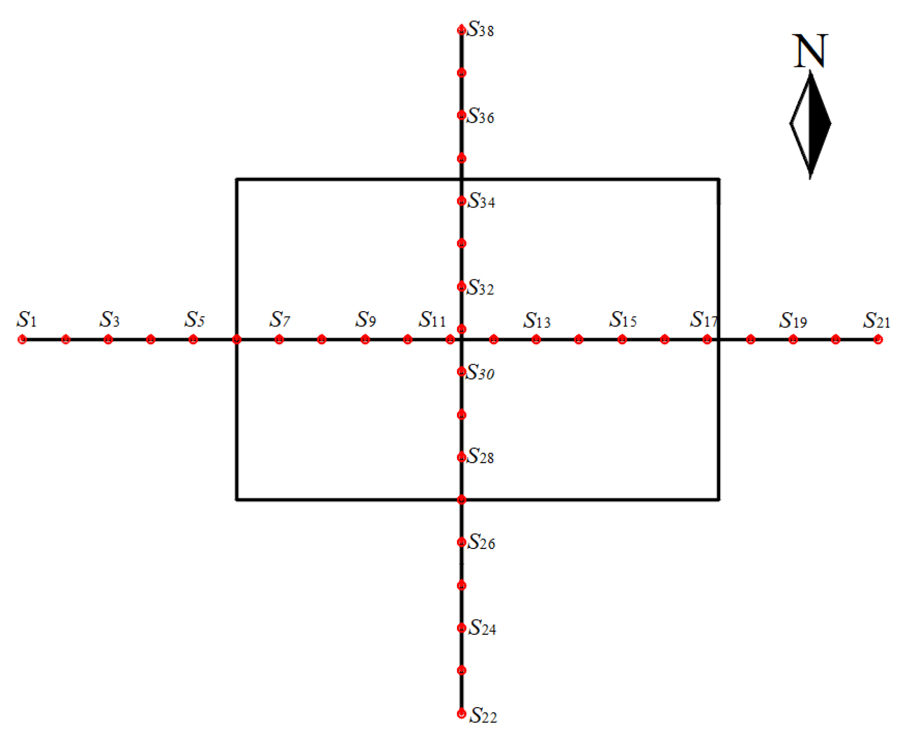
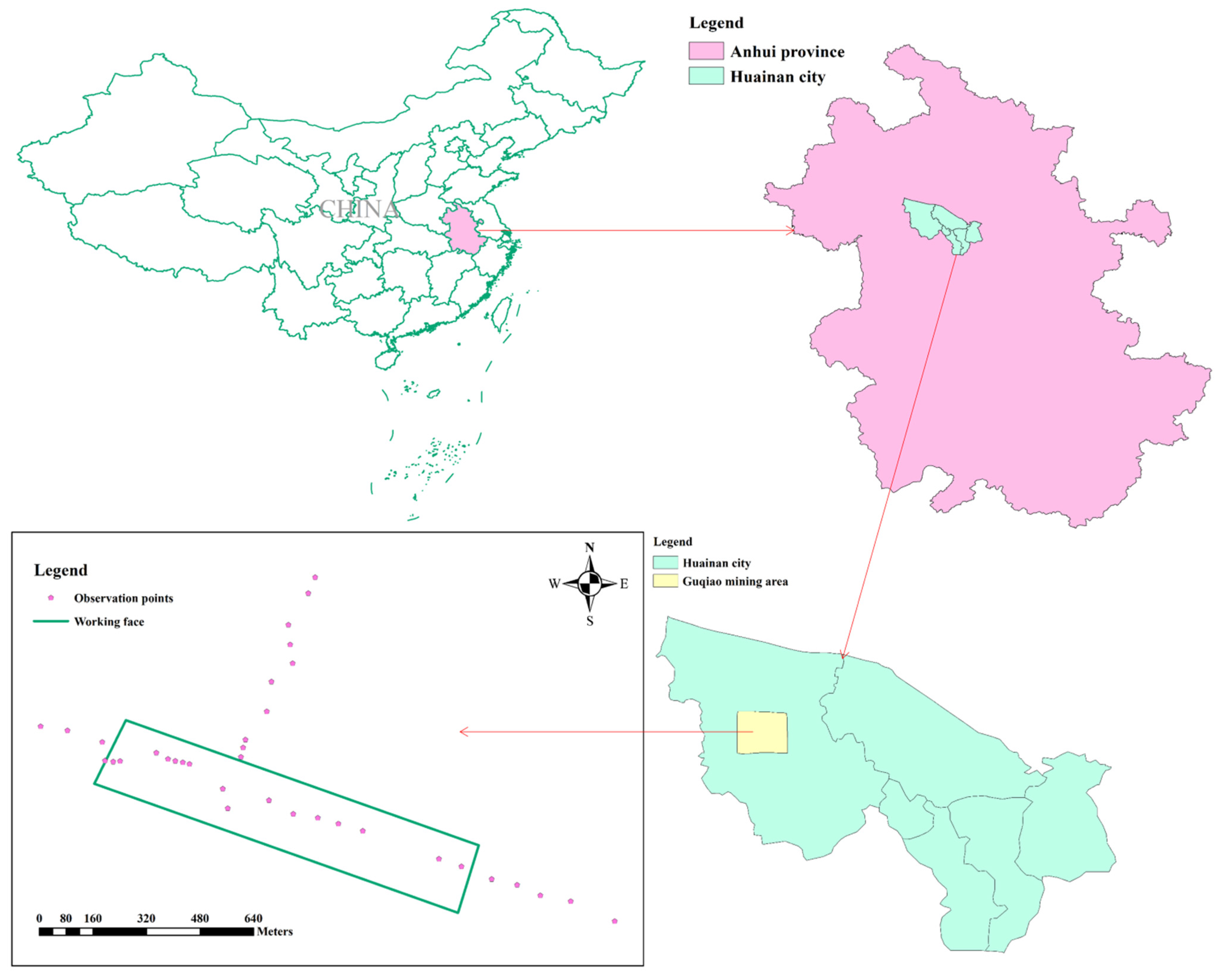
3.1. A Brief Introduction to the Mining Working Face

The probabilistic integral parameters of the simulated working face are given based on the geological mining conditions and empirical parameters of similar locations in the Huainan mining area. The geological conditions for designing a simulated working face are an angle of α = 13°; a mining depth of H = 300 m; a mining thickness m of 3 m; and a length and width of the mined coal seam of D3 = 900 m and D1 = 600 m. The complete collapse method is adopted for roof management. The measurement points are located on the AB section and the CD section, with the interval between the observation points being 80 m. The length of the AB observation line is 1600 m, and a total of 21 observation points are set on the line (S1~S21); the length of the CD observation line is 1280 m, and a total of 17 observation points are set on the line (S22~S38). Figure 2 presents a brief introduction to the mining working face and observation points.

3.2. Overview of Data for Simulated Experimental Geological Mining Conditions

In order to demonstrate that the proposed method has the ability to resist interference from gross errors in the measurement data, and to determine whether this method has advantages over traditional genetic algorithms (GAs), the following simulation experiment was designed. The subsidence of points was calculated using the PIM (q = 0.65; tanβ = 1.5; θ = 86.5°; S1 = S2 = S3 = S4 = 45 m), and the subsidence was calculated using the simulated measured data. Then, two observation points were selected at the edge of the subsidence curve (Plan 1), the inflection point of the subsidence curve (Plan 2), and the Wmax (Plan 3), respectively, and gross errors were added (with a gross error of 0.15Wmax). On this basis, the parameter was inverted using a traditional genetic algorithm and this method (k = 0.1), and the inversion parameter values were compared with the design value. The accuracy evaluation of the parameters obtained using the two inversion methods was performed using Equation (10).
R M S E = i = 1 j ( W r i W p i ) 2 j

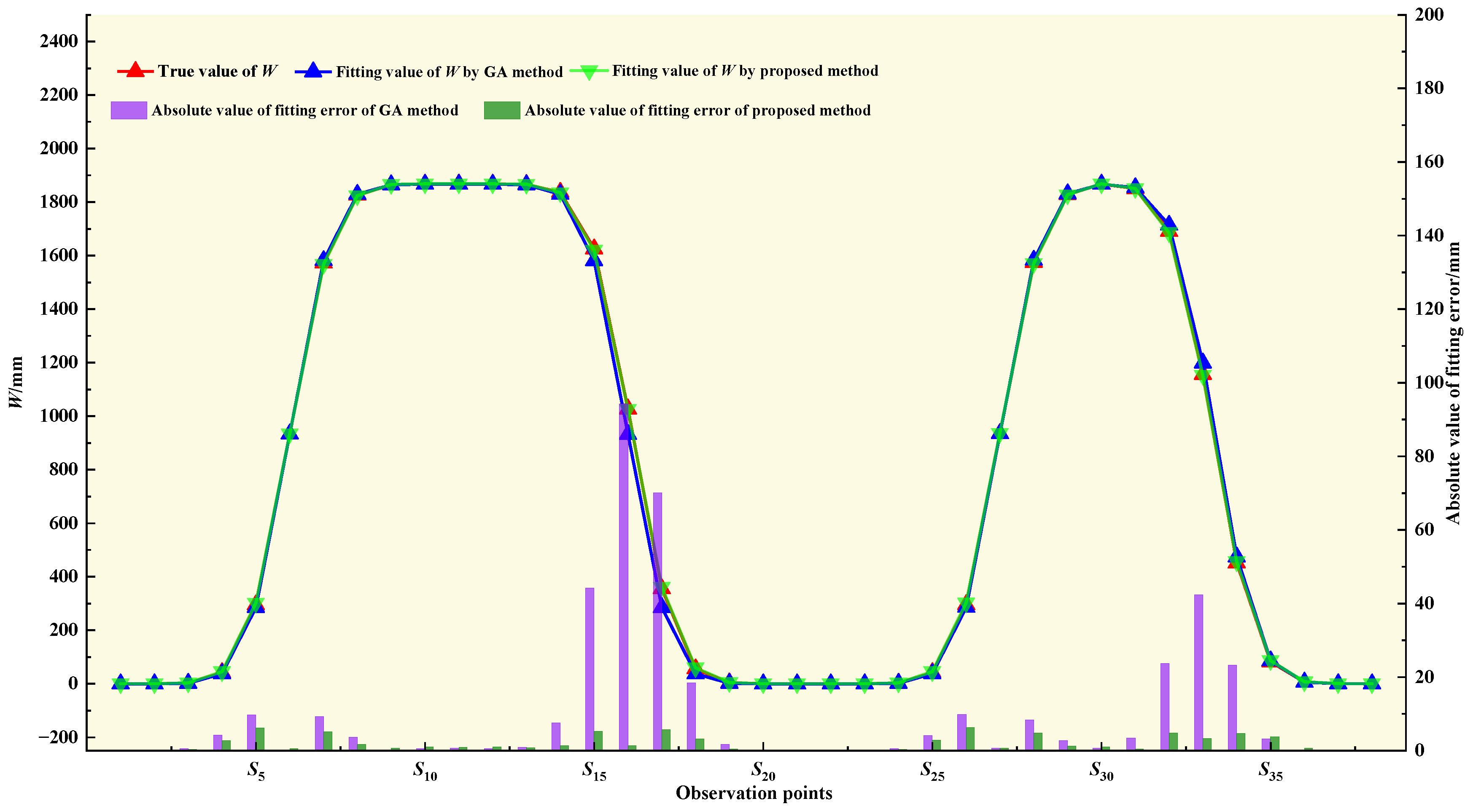
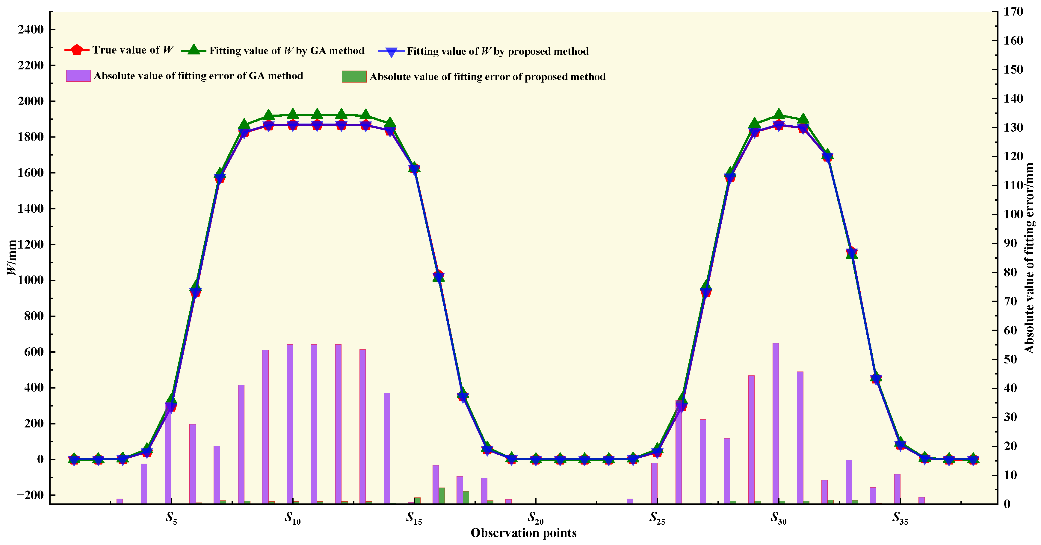
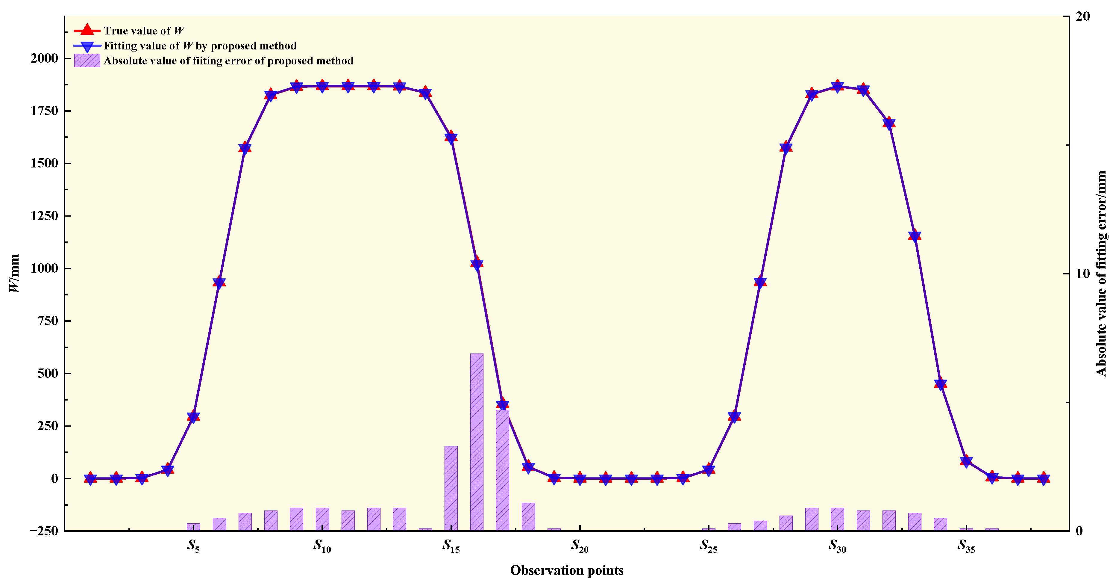
3.3. Simulation Application Experiment and Results

To ensure the stability of parameter inversion and reduce the impact of accidental errors, 50 inversion experiments were performed in each plan, and the inversion values (IVs) of the probability integral parameters were averaged. Table 1 shows the average value, relative error (RE), and fitting RMSE of the parameters in the simulation experiments.
From Table 1, it can be seen that when there are gross errors at three different positions on the subsidence curve, the RMSE (GA) parameter inversion results are 22.5 mm, 33.8 mm, and 28.7 mm, respectively. The relative error of the parameter is 11.43%, 23.73%, and 10.66%. The RMSE of the proposed parameter inversion method is 2.8 mm, 1.7 mm, and 1.4 mm, respectively, and the maximum RE is 4.61%, 1.24%, and 2.67%, respectively. The RMSE and maximum RE of the parameter inversion proposed method are significantly smaller than for the GA. Moreover, the RMSE of the proposed parameter inversion method is reduced by 19.7 mm, 32.1 mm, and 27.3 mm, respectively, compared with the GA. The result of the parameter inversion using this method is closer to the actual value. This indicates that this method is resistant to errors and can reduce the effects of gross errors, ensuring stability and reliability.
In order to verify the accuracy of the probability integral parameters obtained from the inversion of the three schemes for predicting the subsidence of the basin, the parameters of the three experimental schemes and PIM model were used and the subsidence prediction values were obtained. The subsidence predicted by the three schemes was compared with the actual subsidence, as shown in Figure 3, Figure 4 and Figure 5.
From Figure 3, Figure 4 and Figure 5, it can be seen that when observations with gross errors appear at the edge, the maximum absolute errors between the predicted subsidence and actual subsidence for the GA and the proposed method are 94.2 mm and 6.2 mm, respectively. Compared to other locations with gross errors, the impact of the GA is relatively small at this time. When observations with gross errors appear at inflection points and maximum values, the RMSE of the GA is significantly greater than the RMSE of the proposed approach. These results indicate that the anti-gross error performance of this method is more significant, and the RMSE is smaller.

4. 1312(1) Working Face Experiment

4.1. A Brief Introduction to the 1312(1) Working Face

In this study, the 1312(1) working face (located in Guqiao Town, Huainan City, Anhui Province, China) was selected for the experimental research. The parameters of the mine are an angle of α = 5°; a mining depth of H = 528 m; a mining thickness m of 3.3 m; and a length and width of the working surface of D3 = 620 m and D1 = 205 m. The main body of the observation line is arranged in the strike direction, with the observation points being spaced at 30 m. The main body of the inclination observation line is located 310 m away from the start-mining line and 205 m away from the stop-mining line. Taking into account the terrain conditions above the working surface, the inclination observation line is set as a half observation line. Figure 6 shows the study area and the observation points.

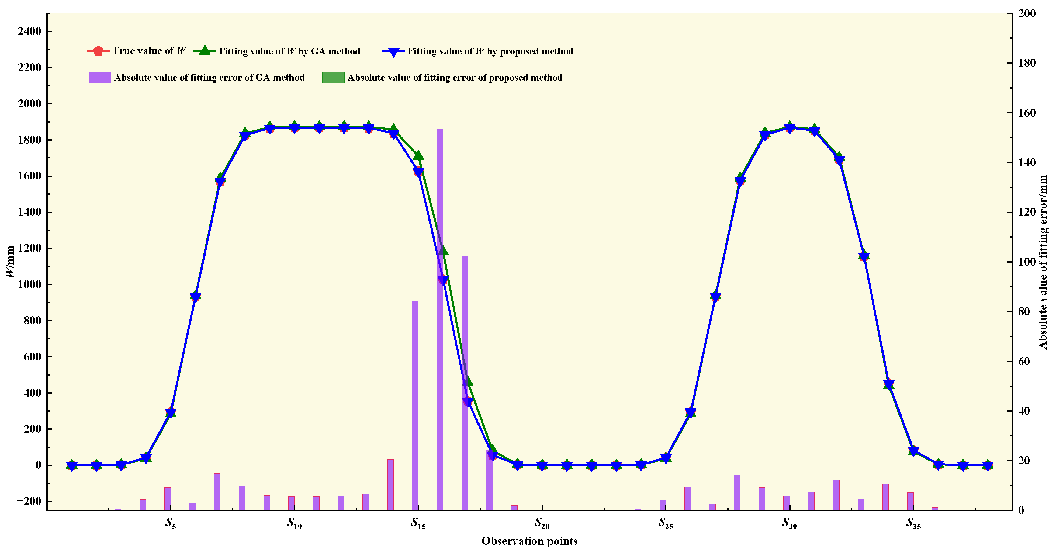
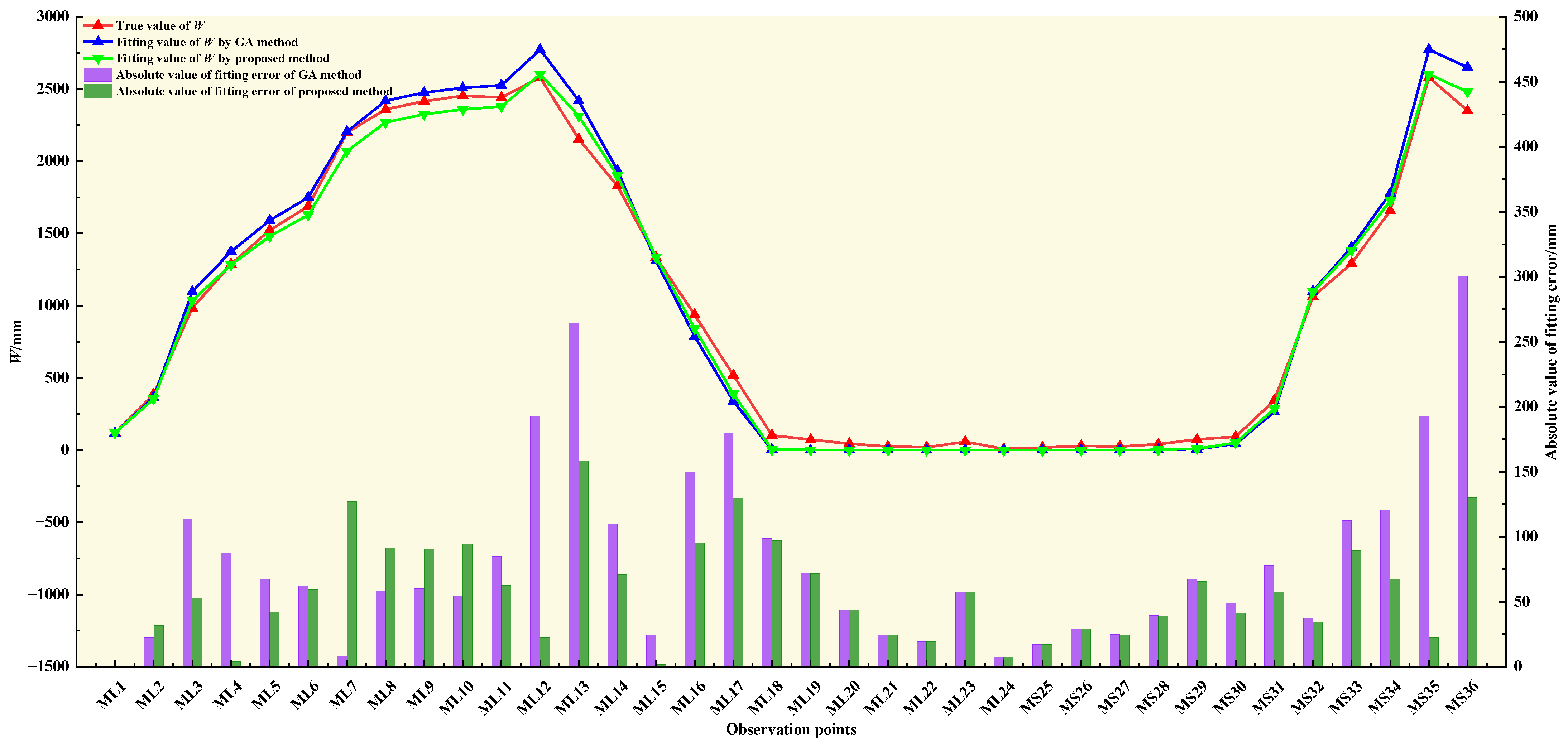
4.2. Engineering Application Experiments and Results

The measured subsidence of 24 points (ML01~ML24) and 12 observation points (MS25~MS36) were selected as the experimental data. Two plans were used to invert the parameters of 13121(1). In the first plan, the PIM parameter inversion is performed using the GA and the measured data without adding coarse errors, and the result is used as the reference value. Three points are selected near the inflection point in the measured subsidence curve data and gross errors are added (two points are selected on the strike observation line; one point is selected on the inclination observation line; and a gross error of 500 mm is added for each point), and then the GA is used to invert the parameters. In the second engineering application plan, three points are selected at Wmax in the measured subsidence curve data and gross errors are added (a gross error of 500 mm is added for each point), and then the GA and the proposed method are used to invert the parameters of the PIM. To ensure that the inversion results are not affected by accidental errors, both schemes perform 50 inversions, and the average value is selected as the result. Table 2 shows the mean and fitting RMSE of the result.
From Table 2, we can see that when gross errors are added near the inflection point and Wmax, the RMSE values of the PIM parameters inverted using the traditional GA are 101.2 mm and 107.3 mm, respectively, while the RMSE values of the parameters inverted using the proposed method are 76.8 mm and 69.8 mm, respectively. In the experiments involving the introduction of two sets of gross errors, the RMSE of the proposed method is reduced by 24.4 mm and 37.5 mm, respectively, compared to that of the traditional genetic algorithm. The proposed method demonstrates better resistance to gross errors compared to the traditional genetic algorithm.
To verify the precision of the parameters obtained from the inversion of the two plans for predicting the subsidence of the basin, the parameters from both plans and the PIM were used. The subsidence values predicted by the two plans were compared with the actual subsidence values, and the results are shown in Figure 7 and Figure 8.
From Figure 7 and Figure 8, it can be seen that when gross errors are added near the inflection point and maximum value, the maximum fitting errors of the parameters inverted using the traditional GA are 225.3 mm and 300.5 mm, respectively. The maximum fitting errors of the parameters inverted using the proposed method are 176.6 mm and 158.5 mm, respectively. The above analysis indicates that the proposed method has the advantage of higher accuracy in inverting probability integral parameters compared to traditional genetic algorithms.

5. Discussion

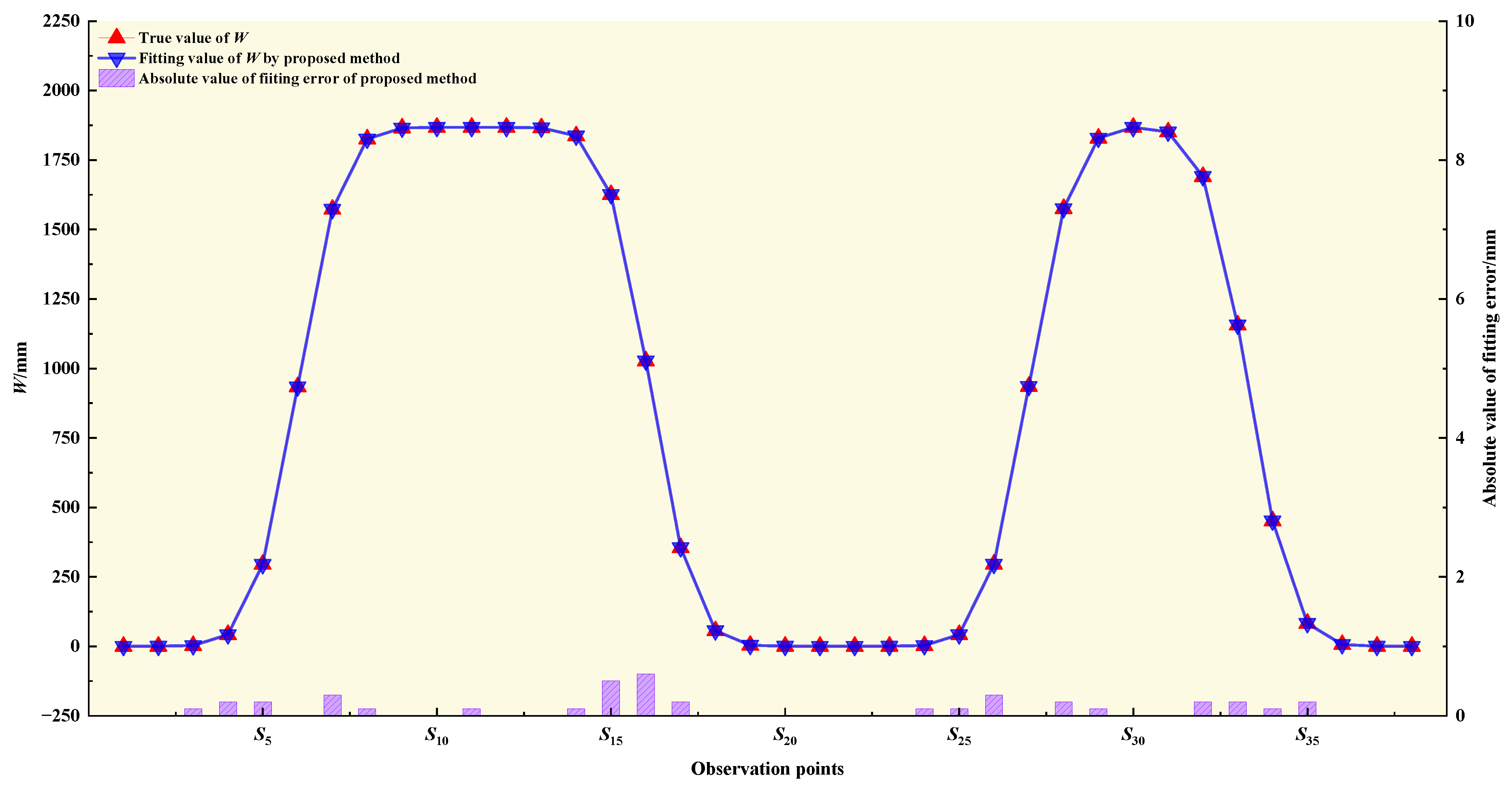
5.1. The Impact of Changes in k Value on the Proposed Method

Based on the geological condition parameters and probability integration method parameters set in the simulation experiment in Section 3, five different k values were set in the experiments performed with gross errors near the edge, inflection point, and maximum subsidence value, respectively. The parameter inversion experiments were performed separately under five different k values. The fitting RMSE of the subsidence values and the relative error of the parameters were used as indicators for evaluating the inversion accuracy. Table 3, Table 4 and Table 5 present the experimental results.
According to Table 3, Table 4 and Table 5, the parameter inversion results for introducing gross errors at three different positions are as follows: when k = 10, the maximum RE values of the parameter inversion results are 6.74%, 8.45%, and 5.57%, respectively, and the RMSE values are 15.2 mm, 18.8 mm, and 25.8 mm, respectively. When k = 1, the maximum RE values of the parameter inversion results are 3.78%, 5.65%, and 3.83%, respectively, and the RMSE values are 1.6 mm, 9.2 mm, and 5.0 mm, respectively. When k = 0.1, the maximum RE values of the parameter inversion results are 2.67%, 4.61%, and 1.24%, respectively, and the RMSE values are 1.4 mm, 2.8 mm, and 1.7 mm, respectively. When k = 0.01, the maximum RE values of the parameter inversion results are 2.94%, 3.24%, and 3.77%, respectively, and the RMSE values are 7.5 mm, 3.9 mm, and 5.8 mm, respectively. When k = 0.001, the maximum RE values of the parameter inversion results are 5.29%, 4.88% and 3.07%, respectively, and the RMSE values are 12.9 mm, 4.8 mm and 2.8 mm, respectively. From these results, it can be concluded that the accuracy of the parameter inversion is relatively limited due to the change in k. As k decreases, the overall trend of the accuracy of parameter inversion shows a pattern of first decreasing, then increasing. When the value of k is set to 0.1, the proposed method has the highest accuracy in inverting the parameters of the PIM. Therefore, in the aforementioned simulation experiments, k was selected as 0.1.

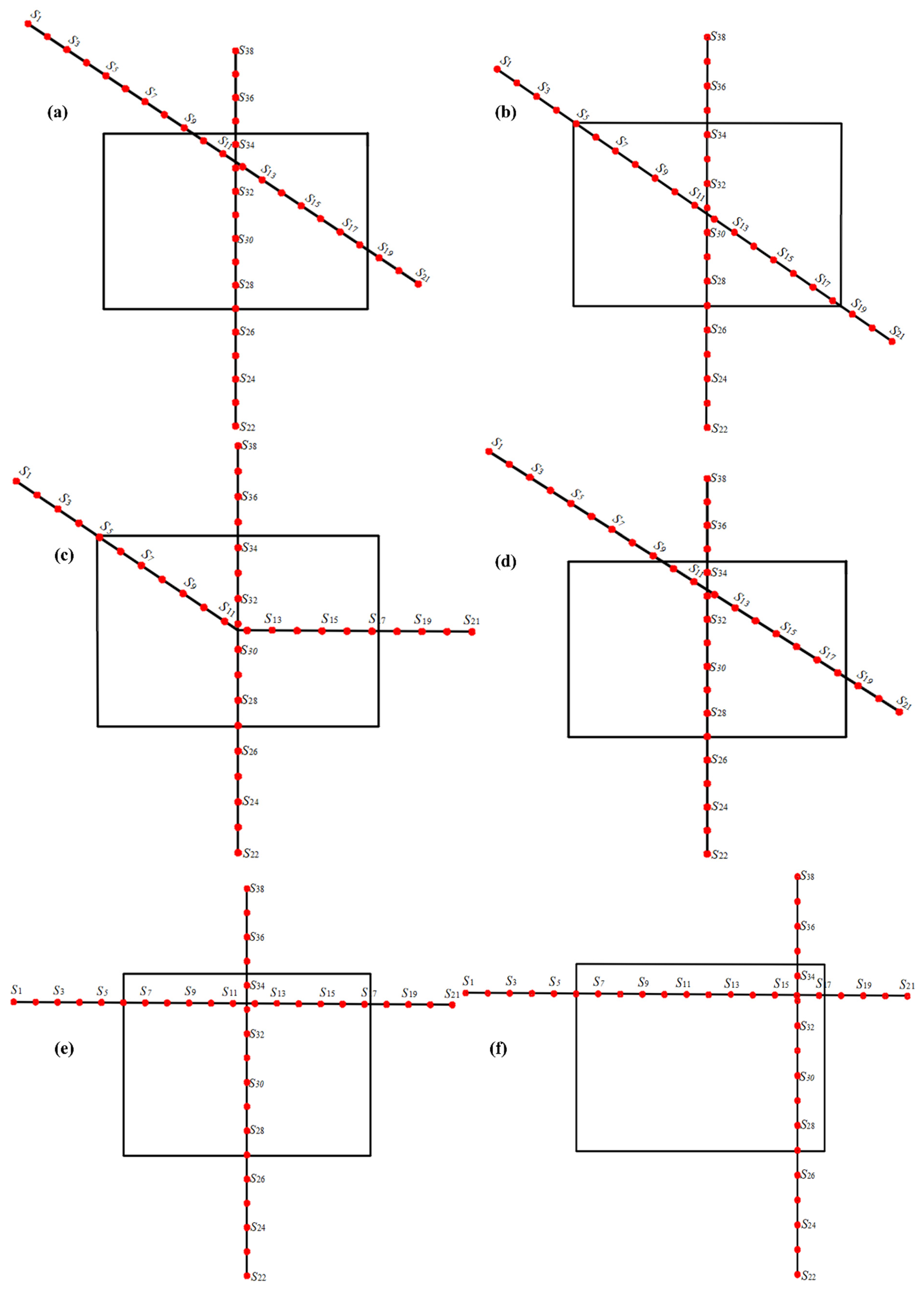
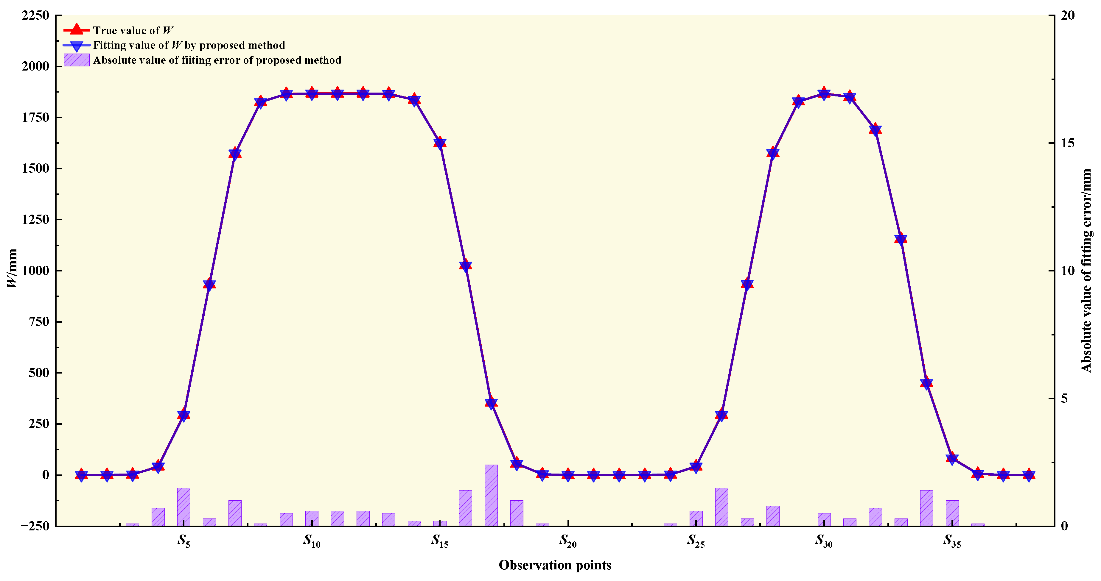
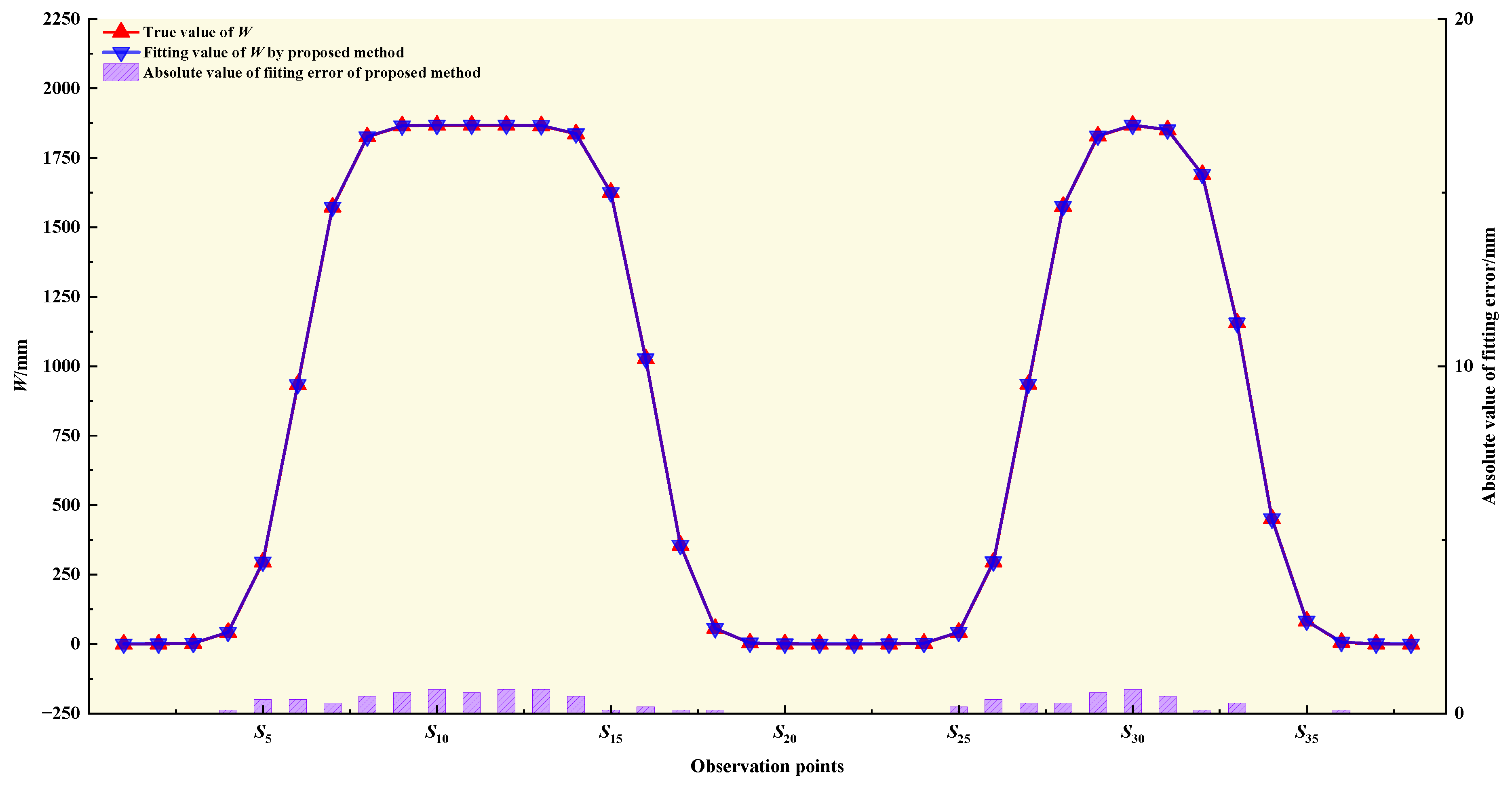
5.2. The Influence of Different Layout Forms of Survey Lines on Parameter Inversion

The standard observation line layout in mining subsidence studies is generally two orthogonal observation lines along the strike main section and the inclination main section of the coal seam. However, the actual layout of observation lines is often restricted by conditions such as terrain and buildings, and cannot be arranged into a standard observation line layout form. In the experimental analysis of the influence of different survey lines on the proposed method, the layout schemes of six different line layout patterns are presented in this study, as shown in Figure 9.
Based on the mine parameters and PIM parameters set in the simulation experiment described in Section 3 (k = 0.1), the PIM parameter inversion experiments were performed separately under six different line layout schemes. The fitting RMSE of subsidence and the relative error of the parameters were used as indicators for evaluating the inversion accuracy. Table 6 and Figure 10, Figure 11, Figure 12, Figure 13, Figure 14 and Figure 15 present the experimental results.
From the table and figures, it can be seen that when the observation line layout pattern is as shown in Plans 2, 3, 4, and 5, there is at least one standard observation line, and some observation lines still pass through the maximum subsidence point. At this time, the observation line layout pattern has little impact on the q, β, θ, or overall fitting accuracy. However, it has a significant impact on the inflection point offsets (S1, S2, S3, and S4) and has some impact on the predicted subsidence value near the inflection point. When the layout of the observation line is as shown in Plan 6, none of the observation pass through the location of Wmax. At this time, the impact on the subsidence coefficient q and inflection point offsets (S1, S2, S3, and S4) is relatively large, but the impact on the tan β and θ is still relatively small, and it has a significant impact on the predicted subsidence near the largest subsidence point, significantly reducing the accuracy of the overall model fitting. These results indicate that, to ensure the precision of mining subsidence prediction, priority should be given to the layout of the observation line as standard when setting up the observation points, ensuring that it passes through the maximum subsidence point as far as possible.

6. Conclusions

(1) Compared with traditional genetic algorithms, the proposed method demonstrates a more significant improvement in robustness when faced with gross interference from observations at different locations. The research results indicate that the method proposed in this paper can effectively reduce the influence of gross errors in the parameter inversion process of probability integration. The parameter integration achieved using this method has high accuracy and reliability.
(2) The accuracy of the parameter inversion result is relatively limited due to the change in the k value. When the value of k is set to 0.1, the proposed method has the highest parameter inversion accuracy. As the value of k decreases, the overall accuracy exhibits a trend of first decreasing, then increasing.
(3) The different forms of the observation line layout pattern have little impact on q, tan β, θ, or overall fitting accuracy. However, it has a significant impact on the inflection point offsets (S1, S2, S3, and S4). When neither the strike nor inclination observation lines pass through the maximum subsidence point, there is a significant impact on the subsidence coefficient q, resulting in a significant decrease in overall fitting accuracy.

Author Contributions

Conceptualization, C.J. and L.W.; methodology, W.L.; validation, C.J., L.W. and W.L.; formal analysis, C.J.; investigation, C.J.; resources, L.W.; data curation, L.W.; writing—original draft preparation, C.J.; writing—review and editing, C.J.; visualization, W.L. and X.Z.; supervision, H.T.; project administration, C.J. and H.T.; funding acquisition, C.J. All authors have read and agreed to the published version of the manuscript.

Funding

This work was supported by the Research Project of the Scientific Research Foundation of Education Department of Anhui Province of China (2024AH051819 and 2023AH052224); the Suzhou University Doctoral (Postdoctoral) Research Initiation Fund, under Grant 2022BSK006; the Quality Engineering Project of Suzhou University, under Grant szxy2023jyxm18; the Coal Industry Engineering Research Center of Mining Area Environmental and Disaster Cooperative Monitoring, Anhui University of Science and Technology, under Grant KSXTJC202203; and the Key Laboratory of Aviation–Aerospace–Ground Cooperative Monitoring and Early Warning of Coal Mining-induced Disasters of Anhui Higher Education Institutes, under Grant KLAHEI202304.

Institutional Review Board Statement

Not applicable.

Informed Consent Statement

Not applicable.

Data Availability Statement

The data can be obtained from the corresponding author according to reasonable requirements. The data are not publicly available due to privacy.

Conflicts of Interest

The authors declare no conflict of interest.

Abbreviations

Symbols used in this work:
SymbolMeaning
Wmaxmaximum subsidence value
W ( x ) subsidence value of the strike section of the coal mining working face
W ( y ) subsidence value of the trend profile of the coal mining working face
ds, dtlength and width of unit mining
Mthickness of the mining face in a coal mine
qsubsidence coefficient
αinclination angle of the coal seam
(x,y)coordinates at any point on the surface
Haverage mining depth of the working surface
Tanβmain influence tangent
θgreatest subsidence angle
D1length of inclination of working face
D3length of strike of working face
S1, S2, S3, and S4upper, lower, left, and right inflection point offsets of the working face, respectively
B = [q,tan β,θ,S1,S2,S3,S4]estimated parameter for subsidence using probability integration method
G = [m,H,x,y,α,D3,D1]geological and mining condition parameter of the working face
v j difference between the true value and the fitted value
W r j measured subsidence value
W p j predicted subsidence value
Vminminimum residual sum of squares after adding weights
Piweight of the i-th observation value
jtotal number of observed values

References

  1. Chai, H.; Xu, H.; Hu, J.; Geng, S.; Guan, P.; Ding, Y.; Zhao, Y.; Xu, M.; Chen, L. Application of a Variable Weight Time Function Combined Model in Surface Subsidence Prediction in Goaf Area: A Case Study in China. Appl. Sci. 2024, 14, 1748. [Google Scholar] [CrossRef]
  2. Zhou, D.W.; Wu, K.; Chen, R.L.; Li, L. GPS/terrestrial 3D laser scanner combined monitoring technology for coal mining subsidence: A case study of a coal mining area in Hebei, China. Nat. Hazards 2014, 70, 1197–1208. [Google Scholar] [CrossRef]
  3. Lei, M.; Zhang, T.; Shi, J.; Yu, J. InSAR-CTPIM-Based 3D Deformation Prediction in Coal Mining Areas of the Baisha Reservoir, China. Appl. Sci. 2024, 14, 5199. [Google Scholar] [CrossRef]
  4. He, M.; Wang, Q.; Wu, Q. Innovation and future of mining rock mechanics. J. Rock Mech. Geotech. Eng. 2021, 13, 1–21. [Google Scholar] [CrossRef]
  5. Zhu, Q.; Li, H.; Yang, X.; Shen, Y. Influence analysis of between subsidence and structure evolution in overburden rock under mining. J. China Coal Soc. 2019, 44, 9–17. [Google Scholar]
  6. Fan, H.; Lu, L.; Yao, Y. Method combining probability integration model and a small baseline subset for time series monitoring of mining subsidence. Remote Sens. 2018, 10, 1444. [Google Scholar] [CrossRef]
  7. Li, H.Z.; Guo, G.L.; Zha, J.F.; Wang, T.; Chen, Y.; Yuan, Y.; Huo, W. A new method of regional mining subsidence control for sustainable development in coal areas. Sustainability 2023, 15, 7100. [Google Scholar] [CrossRef]
  8. Hou, Z.X.; Yang, K.M.; Li, Y.R.; Gao, W.; Wang, S.; Ding, X.M.; Li, Y.X. Dynamic prediction model of mining subsidence combined with D-InSAR technical parameter inversion. Environ. Earth Sci. 2022, 81, 307. [Google Scholar] [CrossRef]
  9. Zhang, J.; Zhang, P.; Ji, X.; Li, Y. Prediction of surface subsidence in Gequan coal mine based on probability integral and numerical simulation. Acad. J. Eng. Technol. Sci. 2024, 7, 8–15. [Google Scholar] [CrossRef]
  10. Zhang, L.L.; Cheng, H.; Yao, Z.S.; Wang, X.J. Application of the improved Knothe time function model in the prediction of ground mining subsidence: A case study from Heze City, Shandong Province, China. Appl. Sci. 2020, 10, 3147. [Google Scholar] [CrossRef]
  11. Kim, Y.; Lee, S.S. Application of Artificial Neural Networks in Assessing Mining Subsidence Risk. Appl. Sci. 2020, 10, 1302. [Google Scholar] [CrossRef]
  12. Guo, W.B.; Deng, K.Z.; Zou, Y.F. Artificial Neural Network Model for Predicting Parameters of Probability-Integral Method. J. China Univ. Min. Technol. 2004, 33, 322–326. [Google Scholar]
  13. Shen, Z.; Xu, L.J.; Liu, X.P.; Qin, C.C.; Wang, Z.B. PIM parameters prediction model optimization based on machine learning methods. Bull. Surv. Mapp. 2016, 10, 35–38. [Google Scholar]
  14. Yu, N.F.; Yang, H.C. Optimal selection of prediction parameters for probability-integral method using particle swarm optimization and BP neural network. Sci. Surv. Mapp. 2008, 33, 78–80. [Google Scholar]
  15. LV, W.C.; Huang, H.; Chi, S.S.; Han, B.W. Neural network optimization algorithm for the prediction parameters of PIM. Sci. Surv. Mapp. 2019, 44, 35–41. [Google Scholar]
  16. Li, P.X.; Tan, Z.X.; Yan, L.L.; Deng, K.Z. Calculation method of probability integration method parameters based on Support vector machine. J. China Coal Soc. 2010, 35, 1247–1251. [Google Scholar]
  17. Wang, Z.S.; Deng, K.Z. Parameters identification of PIM based on multi-scale kernel partial least squares regression method. Chin. J. Rock Mech. Eng. 2011, 2, 3863–3870. [Google Scholar]
  18. Yang, J.; Liu, C.; Wang, B. BFGS method based inversion of parameters in probability integral model. J. China Coal Soc. 2019, 44, 3058–3068. [Google Scholar]
  19. Zha, J.F.; Feng, W.K.; Zhu, X.J. Research on Parameters Inversion in PIM by Genetic Algorithm. J. Min. Saf. Eng. 2011, 28, 655–659. [Google Scholar]
  20. Bo, H.Z.; Lu, G.H.; Li, H.Z.; Guo, G.L.; Li, Y.W. Development of a Dynamic Prediction Model for Underground Coal-Mining-Induced Ground Subsidence Based on the Hook Function. Remote Sens. 2024, 16, 377. [Google Scholar] [CrossRef]
  21. Chen, Y.; Tao, Q.X.; Liu, G.L.; Wang, L.Y.; Wang, F.Y. Detailed mining subsidence monitoring combined with InSAR and PIM. Chin. J. Geophys. Chin. Ed. 2021, 64, 3554–3566. [Google Scholar]
  22. Zhang, X.Y.; Tian, Y.P.; Zhang, X.F.; Bai, M.D.; Zhang, Z.T. Use of multiple regression models for predicting the formation of bromoform and dibromochloromethane during ballast water treatment based on an advanced oxidation process. Environ. Pollut. 2019, 254, 113028. [Google Scholar] [CrossRef] [PubMed]
  23. Bian, H.F.; Yang, H.C.; Zhang, S.B. Research on intelligent optimization for predicting parameters of probability-integral method. J. Min. Saf. Eng. 2013, 30, 385–389. [Google Scholar]
  24. Fan, H.D.; Cheng, D.; Deng, K.Z.; Chen, B.Q.; Zhu, C.G. Subsidence monitoring using D-InSAR and probability integral prediction modelling in deep mining areas. Surv. Rev. 2015, 47, 438–445. [Google Scholar] [CrossRef]
  25. Wang, Q.C.; Li, J.; Guo, G.L. Study on analogy analysis on prediction of surface subsidence parameters in mining area of Chongqing City. Coal Sci. Technol. 2018, 46, 196–202. [Google Scholar]
  26. Li, H.; Zheng, J.; Xue, L.; Zhao, X.; Lei, X.Q.; Gong, X. Inversion of Subsidence Parameters and Prediction of Surface Dynamics under Insufficient Mining. J. Min. Sci. 2023, 59, 693–704. [Google Scholar] [CrossRef]
  27. Wei, T.; Guo, G.L.; Li, H.Z.; Wang, L.; Yang, X.S.; Wang, Y.Z. Fusing Minimal Unit Probability Integration Method and Optimized Quantum Annealing for Spatial Location of Coal Goafs. KSCE J. Civ. Eng. 2023, 26, 2381–2391. [Google Scholar] [CrossRef]
  28. Wang, R.; Hao, K.R.; Chen, L.; Wang, T.; Jiang, C.L. A novel hybrid particle swarm optimization using adaptive strategy. Inf. Sci. 2021, 579, 231–250. [Google Scholar] [CrossRef]
  29. Shao, P.; Wu, Z.J.; Peng, H.; Wang, Y.L.; Li, G.Q. An Adaptive Particle Swarm Optimization Using Hybrid Strategy. Commun. Comput. Inf. Sci. 2018, 874, 26–39. [Google Scholar]
  30. Wang, L.; Jiang, C.; Wei, T.; Li, N.; Chi, S.S.; Zha, J.F.; Fang, S.Y. Robust Estimation of Angular Parameters of the Surface Moving Basin Boundary Induced by Coal Mining: A Case of Huainan Mining Area. KSCE J. Civ. Eng. 2020, 24, 266–277. [Google Scholar] [CrossRef]
  31. Wang, F.W.; Zhou, S.J.; Zhou, Q.; Lu, P.H. Comparisons between three methods in initial residuals problem of selecting weight iteration method. Sci. Surv. Mapp. 2015, 40, 18–21. [Google Scholar] [CrossRef]
  32. Li, H.J.; Tang, S.H.; Huang, J. Discussion for the selection of constant in selecting weight iteration method in robust estimation. Sci. Surv. Mapp. 2006, 31, 70–71+76+51. [Google Scholar]
Figure 1. Technical flowchart of method described in this paper.
Applsci 15 08102 g001
Figure 2. Distribution of working faces and observation points.
Applsci 15 08102 g002
Figure 3. Comparison of fitted subsidence values between proposed method and GA (Plan 1).
Applsci 15 08102 g003
Figure 4. Comparison of fitted subsidence values between proposed method and GA (Plan 2).
Applsci 15 08102 g004
Figure 5. Comparison of fitted subsidence values between proposed method and GA (Plan 3).
Applsci 15 08102 g005
Figure 6. Study area and observation points.
Applsci 15 08102 g006
Figure 7. Comparison of fitted subsidence between proposed method and GA (Plan 1).
Applsci 15 08102 g007
Figure 8. Comparison of fitted subsidence between proposed method and GA (Plan 2).
Applsci 15 08102 g008
Figure 9. Schematic diagram of different line layout schemes. (a) Two observation lines pass through the strike and dip profiles, respectively; (b) a standard dip observation line and an oblique observation line (both passing through the maximum subsidence point); (c) a standard dip observation line and half-strike observation line; (d) a standard dip observation line and an oblique observation line (the oblique observation line does not pass through the maximum subsidence point); (e) a standard dip observation line and an observation line parallel to the strike (one parallel observation line does not pass through the maximum subsidence point); (f) an observation line parallel to the strike and an observation line parallel to the dip (not passing through the maximum subsidence point).
Applsci 15 08102 g009
Figure 10. Subsidence fitting of observation point layout scheme. (The results under the Figure 9a).
Applsci 15 08102 g010
Figure 11. Subsidence fitting of observation point layout scheme.(The results under the Figure 9b).
Applsci 15 08102 g011
Figure 12. Subsidence fitting of observation point layout scheme.(The results under the Figure 9c).
Applsci 15 08102 g012
Figure 13. Subsidence fitting of observation point layout scheme. (The results under the Figure 9d).
Applsci 15 08102 g013
Figure 14. Subsidence fitting of observation point layout scheme. (The results under the Figure 9e).
Applsci 15 08102 g014
Figure 15. Subsidence fitting of observation point layout scheme. (The results under the Figure 9f).
Applsci 15 08102 g015
Table 1. Results and accuracy of inversion probability integral parameters.
ParameterDesign ValuePlan 1Plan 2Plan 3
GA MethodProposed MethodGA MethodProposed MethodGA MethodProposed Method
qIV0.640.63950.64050.64170.64000.66000.6403
RE0.08%0.09%0.26%0.00%3.12%0.04%
tan βIV1.51.53221.48041.53391.50001.41711.5013
RE2.15%1.31%2.26%0.00%5.52%0.09%
θIV86.51.532285.593285.247185.976385.560785.6825
RE2.15%1.05%1.45%0.61%1.09%0.95%
S1/mIV4549.931745.230139.764844.800847.228645.1187
RE10.96%0.51%11.63%0.44%4.95%0.26%
S2/mIV4550.144844.829434.320345.199147.018645.5513
RE11.43%0.38%23.73%0.44%4.49%1.23%
S3/mIV4544.320344.917145.727945.557546.587946.2037
RE1.51%0.18%1.62%1.24%3.53%2.67%
S4/mIV4544.320347.072547.175445.475349.798345.3857
RE1.51%4.61%4.83%1.06%10.66%0.86%
RMSE/mm 22.52.833.81.728.71.4
Table 2. Experimental results of the two plans.
ParameterReference ValueEngineering Application Plan 1Engineering Application Plan 2
GA MethodProposed MethodGA MethodProposed Method
qIV1.26721.55331.24041.37981.2889
RE17.94%34.47%27.10%31.91%
tan βIV1.89281.65471.87001.91131.8721
RE12.58%1.20%0.98%1.09%
θIV86.526687.465285.309486.884385.5449
RE1.08%1.41%0.41%1.13%
S1/mIV14.006236.579517.037043.228223.7842
RE161.17%21.64%208.64%69.81%
S2/mIV44.560652.072742.782426.538434.7214
RE16.86%3.99%40.44%22.08%
S3/mIV−2.939810.688615.6669−11.27519.6938
RE463.58%632.92%283.53%429.74%
S4/mIV6.29643.3455−21.316121.0065−4.0305
RE46.87%438.54%233.63%164.01%
RMSE/mm69.7101.276.8107.369.8
Table 3. Results and accuracy of inversion probability integral parameters (Plan 1).
Parameterqtan β θS1/mS2/mS3/mS4/mRMSE/mm
kDesign value0.6400 1.5000 86.5000 45.0000 45.0000 45.0000 45.0000
k = 10IV0.6405 1.6011 85.6798 44.0935 46.3629 45.2836 46.2499 15.2
RE0.08%6.74%−0.95%−2.01%3.03%0.63%2.78%
k = 1IV0.6400 1.5101 85.8538 44.4956 45.7281 46.7030 44.5848 1.6
RE0.00%0.67%−0.75%−1.12%1.62%3.78%−0.92%
k = 0.1IV0.6403 1.5013 85.6825 45.1187 45.5513 46.2037 45.3857 1.4
RE0.04%0.09%0.95%0.26%1.23%2.67%0.86%
k = 0.01IV0.6414 1.5363 85.1924 45.4640 43.7179 45.9748 46.3232 7.5
RE0.22%2.42%−1.51%1.03%−2.85%2.17%2.94%
k = 0.001IV0.6407 1.5794 86.0870 44.7540 44.0796 45.0884 44.7858 12.9
RE0.11%5.29%−0.48%−0.55%−2.05%0.20%−0.48%
Table 4. Results and accuracy of inversion probability integral parameters (Plan 2).
Parameterqtan β θS1/mS2/mS3/mS4/mRMSE/mm
kDesign value0.6400 1.5000 86.5000 45.0000 45.0000 45.0000 45.0000
k = 10IV0.6404 1.6268 86.0113 46.1155 45.3005 43.8490 47.2080 18.8
RE0.06%8.45%−0.56%2.48%0.67%−2.56%4.91%
k = 1IV0.6444 1.5001 85.3051 44.8297 44.3856 43.7977 47.5408 9.2
RE0.69%0.01%−1.38%−0.38%−1.37%−2.67%5.65%
k = 0.1IV0.6405 1.4804 85.5932 45.2301 44.8294 44.9171 47.0725 2.8
RE0.09%1.31%1.05%0.51%0.38%0.18%4.61%
k = 0.01IV0.6390 1.5257 85.2503 43.8192 45.1534 46.4601 46.0842 3.9
RE−0.15%1.71%−1.44%−2.62%0.34%3.24%2.41%
k = 0.001IV0.6368 1.5205 85.6139 43.0816 46.2739 47.1941 44.4129 4.8
RE−0.50%1.37%−1.02%−4.26%2.83%4.88%−1.30%
Table 5. Results and accuracy of inversion probability integral parameters (Plan 3).
Parameterqtan β θS1/mS2/mS3/mS4/mRMSE/mm
kDesign value0.6400 1.5000 86.5000 45.0000 45.0000 45.0000 45.0000
k = 10IV0.6505 1.5557 85.7074 42.4913 45.6933 44.8361 44.8234 25.8
RE1.64%3.72%−0.92%−5.57%1.54%−0.36%−0.39%
k = 1IV0.6427 1.5000 85.4679 43.9696 46.1892 46.7253 45.0778 5.0
RE0.42%0.00%−1.19%−2.29%2.64%3.83%0.17%
k = 0.1IV0.6400 1.5000 85.9763 44.8008 45.1991 45.5575 45.4753 1.7
RE0.00%0.00%0.61%0.44%0.44%1.24%1.06%
k = 0.01IV0.6407 1.5314 86.1272 44.4732 46.4933 43.4665 46.6973 5.8
RE0.11%2.09%−0.43%−1.17%3.32%−3.41%3.77%
k = 0.001IV0.6399 1.5000 85.1070 44.6436 45.1770 45.0159 46.3817 2.8
RE−0.01%0.00%−1.61%−0.79%0.39%0.04%3.07%
Table 6. Results of probability integral parameter inversion with different survey line configurations.
Parameterqtan β θS1/mS2/mS3/mS4/mRMSE/mm
PlanDesign value0.6400 1.5000 86.5000 45.0000 45.0000 45.0000 45.0000
Layout Plan 1IV0.6403 1.4982 84.7213 44.4317 46.8088 45.4997 48.2903 1.2
RE0.05%0.12%2.06%1.26%4.02%1.11%7.31%
Layout Plan 2IV0.6400 1.5008 84.4382 46.1015 43.8334 43.5677 50.5812 0.2
RE0.00%0.05%2.38%2.45%2.59%3.18%12.40%
Layout Plan 3IV0.6398 1.5048 84.9745 43.9372 46.2053 46.0874 46.9935 0.8
RE0.03%0.32%1.76%2.36%2.68%2.42%4.43%
Layout Plan 4IV0.6402 1.4991 85.2291 41.6217 48.4276 44.1853 48.4487 0.4
RE0.03%0.06%1.47%7.51%7.62%1.81%7.66%
Layout Plan 5IV0.6403 1.4996 85.3239 46.7982 43.9935 49.2968 43.0575 1.6
RE0.05%0.03%1.36%4.00%2.24%9.55%4.32%
Layout Plan 6IV0.6128 1.5080 85.9702 39.7584 45.5032 40.3865 45.9748 45.0
RE4.25%0.53%0.61%11.65%1.12%10.25%2.17%
Disclaimer/Publisher’s Note: The statements, opinions and data contained in all publications are solely those of the individual author(s) and contributor(s) and not of MDPI and/or the editor(s). MDPI and/or the editor(s) disclaim responsibility for any injury to people or property resulting from any ideas, methods, instructions or products referred to in the content.

