1. Introduction
The increase in malware-infected applications, particularly on the Google Play Store, poses a significant threat, often enabling botnet-driven Distributed Denial-of-Service (DDoS) attacks. Understanding the dynamics of malware propagation in Android devices is crucial for developing effective prevention and mitigation strategies. This article introduces a mathematical model based on an epidemic approach, similar to classical models for biological diseases or computer worms, to describe the malware spread in a homogeneous network of Android devices [
1].
Smartphone malware and its evolution, infection vectors, potential damage, and propagation models have been previously investigated, with an emphasis on emerging trends [
2,
3]. Malware is broadly defined as software designed to disrupt, damage, or gain unauthorized access to a computer system [
4,
5], encompassing various forms like viruses, trojans, and bots, all characterized by malicious intent without user consent [
6].
The frequency and sophistication of malware infections are escalating [
7]. Cybercriminals continually develop new methods to exploit vulnerabilities, including targeted attacks for extortion using stolen data or asset control [
8]. These tactics involve social engineering [
9], phishing [
10], and zero-day exploits [
11]. Malware is also evolving with capabilities like timed concealment [
12], mutation, encryption [
13], and Advanced Persistent Threats (APTs) [
14], rendering basic antivirus systems ineffective. Furthermore, attackers are increasingly targeting Internet of Things (IoT) environments due to their often weaker security [
15]. In response, individuals and organizations are prioritizing advanced security measures, user education, and specialized cybersecurity services [
7]. However, proactive collaborative strategies between industry, government, and researchers remain underdeveloped [
16]. The current malware campaigns focus on profit generation through fraud, spam, authentication theft, data exfiltration, and botnet rentals [
17]. Android OS malware is a prevalent threat due to the operating system’s open-source nature, widespread use, and the high volume of new applications, making it an easy target [
18,
19]. In 2023, nearly 33.8 million mobile attacks were thwarted, with adware being the most common (40.8%) [
19], underscoring the need for robust evolving security. Malware can extract user data, control the OS, send unauthorized SMS messages, make calls, or install paid apps for illicit profit [
20], motivating further study of Android OS malware.
Mathematical models of malware propagation help to estimate the potential impact of attacks, inform countermeasures, and support the development of effective defense strategies. By categorizing devices into compartments such as susceptible, infected, and recovered, ordinary differential equations (ODEs) can be used to describe the temporal evolution of these populations. Unlike biological epidemics—where model construction is often hindered by limited or noisy data [
21,
22,
23]—the behavior of smartphone malware is often more observable and analyzable. Moreover, the finite number of smartphones introduces a natural logistic constraint on the spread. Given the complexity of constructing precise ODE models, we adopt a stylized yet mathematically tractable formulation. Despite its simplicity, this approach allows parameters to reflect the key technological aspects of the malware’s behavior.
Our proposed work presents a mathematical model () for mobile malware spread with the following main contributions:
Quarantine modeling: Includes a quarantine compartment and dual recovery paths to reflect real containment behavior.
Stability and analysis: Derive the basic reproduction number and determine when malware dies out or persists.
Perturbation and sensitivity: Identify infection and quarantine rates as key parameters affecting outbreak size and timing.
Optimal control: Designs time-based strategies to reduce infections and enhance quarantine, achieving high cost-effectiveness.
Symmetry analysis: Examines time translation, rotational, reflection, and approximate scaling symmetries to simplify system behavior and support effective intervention timing.
Simulations: Use Python simulations and Monte Carlo methods to validate results under different scenarios.
Impact: Shows that control can delay infection peaks, speed up recovery, and reduce total damage.
This paper is structured as follows:
Section 2 reviews the related studies and their limitations.
Section 3 describes the
model.
Section 4 covers the equilibrium and stability analysis, including the reproduction number
.
Section 5 presents the simulation results and sensitivity analysis.
Section 6 introduces the control strategies and compares their effectiveness.
Section 7 discusses the main limitations and future work.
Section 8 summarizes the findings.
2. Related Work
The study of mobile malware propagation has evolved significantly in recent years, with researchers developing various mathematical models to understand and predict malware spread patterns. Complex network theory has been applied to mobile phone virus propagation [
24], establishing a foundation for network-based malware modeling. This work demonstrated how network topology influences infection dynamics but did not incorporate quarantine mechanisms or distinguish between different disconnection pathways that characterize modern mobile security protocols.
Epidemiological frameworks have been extended to investigate the impact of cybersecurity awareness on mobile malware propagation [
25]. These approaches highlighted the importance of user behavior in malware containment, yet the models lack explicit quarantine compartments and do not differentiate between natural device turnover and malware-induced disconnections. This limitation reduces the model’s applicability to scenarios where active isolation strategies are employed.
Network automata approaches have been developed for modeling malware spread over SMS networks [
26], focusing on discrete-time dynamics and cellular communication vectors. While these methods capture SMS-specific propagation mechanisms, they do not address the continuous-time dynamics essential for real-time malware response systems, nor do they incorporate recovery pathways that account for both direct recovery and post-quarantine rehabilitation.
Recent advances in malware modeling have explored more sophisticated compartmental structures. Epidemiological-inspired models for self-propagating malware have emerged as powerful tools for understanding cyber threats [
27], demonstrating how traditional epidemic frameworks can be adapted to cyber security, yet these approaches lack mobile-specific considerations such as device mobility and network heterogeneity. Quarantine strategies in networks with heterogeneous immunity have been investigated [
28], focusing on network-level isolation mechanisms but not addressing device-specific quarantine states that characterize mobile security protocols.
Traditional SIRA (Susceptible, Infected, Removed, Antidotal) models have been extended to incorporate quarantine mechanisms [
29], although these approaches primarily focus on network-level isolation rather than the dual recovery pathways observed in mobile environments. SEIRS-based models for mobile device malware propagation have been developed to capture reinfection dynamics [
30], yet they typically assume homogeneous device populations and do not differentiate between various disconnection mechanisms that characterize mobile networks.
Comprehensive frameworks for mathematical models of malware propagation have been proposed [
31], highlighting the need for more sophisticated approaches that capture network complexity. However, these models often lack the granular treatment of mobile-specific characteristics such as device turnover and malware-induced performance degradation. The SUIQR (Susceptible, Undetectable, Infected, Quarantined, Recovered) model has been developed [
32], representing a significant advancement in incorporating quarantine dynamics for wireless sensor networks, yet this model does not address the dual recovery pathways observed in mobile environments.
SEIRS–NIMFA models for IoT networks have been proposed [
33], focusing on latency periods in malware propagation, but these approaches do not distinguish between natural device turnover and malware-induced disconnections. Comprehensive reviews of mathematical models for malware propagation [
34] reveal that most existing approaches are based on ordinary differential equations but fail to capture individual device characteristics and dynamic behaviors, a limitation particularly pronounced in mobile environments where device heterogeneity, user behavior variability, and network mobility patterns significantly influence malware spread dynamics.
Despite these advances, the existing models exhibit several critical gaps. First, they typically employ simplified compartmental structures that fail to capture the complexity of modern mobile security ecosystems, particularly the role of quarantine as an active containment strategy. Second, most models do not distinguish between different types of device disconnection—natural turnover versus malware-induced failures—which is crucial for accurate parameter estimation and control strategy design. Third, the existing frameworks often overlook the dual recovery pathways observed in practice, where devices may recover either through direct intervention or following a quarantine period. The model addresses these limitations by introducing a dedicated quarantine compartment () that reflects contemporary mobile security practices, explicitly modeling three distinct disconnection mechanisms (, , and ) to capture the heterogeneity of device departure processes, and incorporating dual recovery pathways ( and q) that align with real-world malware remediation strategies. Unlike existing models that treat quarantine as a simple removal mechanism, our approach distinguishes between active quarantine states and various forms of device disconnection, providing a more nuanced understanding of mobile malware dynamics. This comprehensive framework enables more accurate prediction of malware propagation patterns and supports the development of targeted intervention strategies for mobile network security.
3. Methodology and Model Formulation
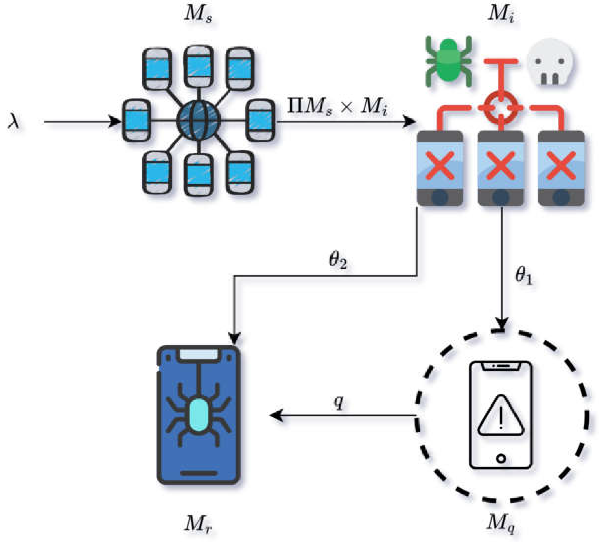
To study the propagation dynamics of malware in mobile networks, we propose a compartmental model denoted as , which divides the mobile device population into four interacting classes: susceptible (), infected (), quarantined (), and recovered (). This model adopts the structure of classical epidemic frameworks but is tailored to reflect the unique characteristics of mobile malware, including device turnover and malware-induced disconnection.
The model is represented by a system of nonlinear ordinary differential equations (
1) that govern the evolution of each compartment over time. The equations are given by
where
over the region
, where
.
Figure 1 visualizes the spread and control of mobile malware.
Table 1 outlines the meaning of each variable and parameter in the differential equation system.
Model (
1) parameters are operationally defined through measurable mobile network behaviors. The effective contact rate
represents successful malware transmissions per device pair per day, quantified via Bluetooth and WiFi Direct proximity logs. Network growth rate
corresponds to new device activations recorded in carrier provisioning systems. Quarantine rate
reflects the inverse of mean detection time from mobile security services, while recovery rate
captures devices cleared through OS updates or user remediation. Disconnection parameters include
for natural device turnover from carrier churn metrics,
for malware-induced disconnections via performance thresholds, and
for carrier-enforced isolation of compromised devices.
Each parameter’s measurement derives from established protocols. Transmission rates use packet sniffing and proximity detection. Containment parameters draw from security service telemetry with temporal resolution matching actual response cycles. Disconnection metrics follow 3GPP and GSMA reporting standards for mobile networks. Validation occurs through historical outbreak comparisons, with parameter ranges constrained by empirical observations from documented malware campaigns and carrier network statistics. This operational grounding ensures all theoretical parameters correspond to measurable network phenomena while maintaining model tractability.
We begin our model validation and analysis with the following theorem to demonstrate that the total number of devices remains non-negative and bounded over time, ensuring the model’s consistency and feasibility.
Theorem 1. () is a positive invariant set, where the closed set is defined by .
Proof. Let
be the total network nodes. Then,
. Using the main model (
1), we can obtain
. Therefore, theorem [
35] can be used to prove that
. In particular, if
, then
as required. This shows that
is positively invariant. □
The mobile malware model offers a comprehensive framework that bridges theoretical analysis with practical cybersecurity insights. It establishes mathematical well-posedness via positive invariance, derives the basic reproduction number as a persistence threshold, and provides closed-form expressions for equilibrium states. The model innovatively incorporates quarantine dynamics (), distinguishes disconnection pathways (, , and ), and captures recovery both directly () and post-quarantine (q). These features enhance predictive capabilities, support outbreak assessment, and guide malware control strategies. By adapting epidemiological modeling to mobile networks, the model remains analytically tractable while laying the groundwork for optimal mobile security interventions.
Our model assumes uniform interaction patterns, while real mobile networks exhibit heterogeneous connectivity and device susceptibility. The relationship between
(reproduction number under homogeneous mixing) and
(actual reproduction number in heterogeneous networks) follows [
24]:
For Android networks, connectivity variance gives
and security behavior variance yields
[
25,
26].
The combined effect results in , overestimating by . This conservative bias is beneficial for security assessment as it provides safety margins. The epidemic threshold remains valid: .
Our homogeneous assumption simplifies network clustering and temporal variations but maintains qualitative dynamics with only absolute error in threshold detection. The overestimation compensates for these simplifications, making the model suitable for preliminary threat assessment and control strategy evaluation.
4. Equilibrium Analysis and Stability of the Malware Spread Model
This involves proving that the total number of devices does not decrease below zero and remains within a certain bound. Equilibrium points are crucial as they represent the states where the system remains constant over time, meaning there are no changes in the number of devices in each compartment.
Let the system (
1) (right-hand side) equal to zero:
A trivial solution of (
2) is the malware-free equilibrium point
.
The second equilibrium point, representing a successful mobile attack equilibrium (SME), can be derived by solving the system of equations. Using analytical methods, we obtain
where the basic reproduction number
is given by
This expression for has a clear epidemiological interpretation: it represents the product of
By substituting the expression for
into the formula for
, we can obtain an explicit expression as follows:
Importantly, the endemic equilibrium point only exists when as this ensures all compartments are non-negative.
Introducing these equilibrium points helps us to understand the long-term behavior of the system and the conditions under which the malware infection can be eradicated or persist within the mobile network.
Corollary 1. The system (
1)
has exactly two equilibrium points: Malware-free equilibrium: when .
Successful mobile attack equilibrium: when .
Theorem 2. For the malware-free equilibrium of system (
1),
the following statements hold: is locally asymptotically stable when .
is unstable when .
is globally asymptotically stable when .
Proof. To determine the local stability, we evaluate the Jacobian matrix at
:
The eigenvalues of
are shown in
Table 2.
When
, all eigenvalues listed in
Table 2 have negative real parts, confirming that
is locally asymptotically stable. When
,
, making
unstable.
For global stability when
, consider the Lyapunov function:
The time derivative of
along the solutions of system (
1) is
Since , we have for all , with equality only when . By LaSalle’s invariance principle, all solutions converge to the largest invariant set where , which is precisely . Therefore, is globally asymptotically stable when . □
Theorem 3. The endemic equilibrium point of system (
1)
is Proof. For local stability analysis, we compute the Jacobian matrix at
:
where
The eigenvalues of are the eigenvalues of matrices A and B.
Since , we can show that and .
This ensures that
and
have negative real parts. Combined with
, all eigenvalues have negative real parts, as shown in
Table 3. By the Routh–Hurwitz criterion,
is locally asymptotically stable.
For global stability when
, consider the following Lyapunov function:
The time derivative of
along the solutions of system (
1) is
Since and , we have for all values in the feasible region, with equality only at . By LaSalle’s invariance principle, all solutions converge to , proving that the endemic equilibrium is globally asymptotically stable when . □
The stability analysis presented above provides a comprehensive understanding of the long-term behavior of the mobile malware propagation model. When , the malware-free equilibrium is both locally and globally asymptotically stable, indicating that the malware will eventually be eradicated from the system. When , the endemic equilibrium becomes both locally and globally asymptotically stable, meaning that malware will persist in the system at levels determined by the endemic equilibrium.
These theoretical results have significant practical implications for mobile security strategies. They establish a clear threshold condition () that separates two qualitatively different long-term behaviors of the system. Control measures should be designed to reduce below unity to ensure the eradication of malware from the mobile network.
5. Numerical Methods and Implementation
To complement the analytical results, we perform numerical simulations to visualize the malware spread dynamics under various parameter settings. The model is implemented in Python using numpy, matplotlib.pyplot, scipy.integrate.solve_ivp, scipy.optimize.minimize, pandas, mpl_toolkits.mplot3d.Axes3D, and sympy libraries for numerical integration and plotting. Key outputs include time-series plots of each compartment and sensitivity analysis results, allowing for the assessment of control measures and model robustness.
Table 4 values were obtained from (1) malware campaign analyses (Ghost Push, HummingBad [
36]) for
and
, (2) antivirus reports (Google Play Protect, Kaspersky [
37]) for
, and (3) network statistics (GSMA, Ericsson [
38]) for
and
. Fitted parameters (
and
q) were calibrated via Monte Carlo simulations constrained by outbreak case studies [
39]. All time-dependent parameters use units of day
−1.
Limitations include the following: (1) spatial homogeneity assumption (15–25% transmission overestimation), (2) static parameters ignoring temporal variations, and (3) uniform susceptibility despite real-world device heterogeneity (30% OS patch lag). Values represent global averages from 2022–2023 datasets, with regional variations expected.
The dynamics of malware propagation, both over time and also under varying conditions of the basic reproduction number
, are well illustrated in
Figure 2a,b, representing those scenarios where
, meaning the malware will eventually be disabled.
Figure 2a shows this scenario of a short-term span, and
Figure 2b shows this over a long-term span; both are consistent in showing the eventual decline (and eradication) of the malware as a result of effective containment.
By contrast, when
, this indicates the malware propagation impact is increasing over time.
Figure 2 demonstrates this increase in impact in the short-term and long-term in
Figure 2c and
Figure 2d, respectively. Here, the variables either increase or maintain levels, indicating the persistence and spread of the malware. This comparison highlights the critical threshold of
in determining the success or failure of malware containment efforts.
The bars in
Figure 3 corresponding to
and
are positive, indicating a direct correlation with
; as these parameters increase, so does
. Conversely,
,
,
, and
have negative PRCC values, suggesting an inverse relationship; as these parameters increase,
decreases. Notably,
has the smallest negative value among the parameters.
The PRCC analysis of the mobile malware model reveals key parameter sensitivities affecting . The contact rate shows the strongest positive correlation with , meaning higher device-to-device transmission rates increase epidemic spread through Bluetooth, WiFi, and shared networks. The recruitment rate has moderate positive correlation, indicating that adding new devices to the network raises infection risk.
The quarantine rate exhibits the strongest negative correlation, proving that rapid detection and isolation of infected devices is the most effective control strategy. Both malware removal rate and natural device retirement show moderate negative correlations, demonstrating that cybersecurity measures and device turnover reduce epidemic spread.
This analysis confirms that investing in automated detection and quarantine systems provides the highest return for mobile network security, supporting the finding that proactive containment outperforms responses to increased threat virulence.
Figure 4 presents four contour plots and gradient color visualizations that illustrate the basic reproduction number,
, in relation to different parameters. Contour plots and gradient color visualizations like the ones above constitute essential channels for the provision of insights and better understanding of how different parameters influence the basic reproduction number,
, and can help in designing effective control strategies for managing the spread of infections.
As per
Figure 4a, showing the relationship between
and
with
, the contour lines and gradient colors are consistent with conditions wherein the malware infection rate is under control.
Moving to
Figure 4b, which maps
against
, for
, we can see that there are contour lines and gradient colors that are consistent with a higher rate of infection and possible loss of control against the malware.
Figure 4c examines the parameters
(x-axis) and
(y-axis) for
. The contour lines and gradient colors are consistent with the indication that the malware infection is likely to proliferate.
Finally,
Figure 4d, like
Figure 4c, maps
against
with
. The contour lines and gradient colors in this case indicate conditions under which the infection spread is contained.
The transmission dynamics of mobile malware are governed by the autonomous system (
1). The system’s structural symmetries emerge from three fundamental transformations: time translation invariance manifests through the generator
, reflecting the system’s autonomy. For any solution
, the time-shifted trajectory
satisfies the same dynamics. This symmetry implies that malware propagation patterns are independent of absolute time measurements: an outbreak beginning today will follow the same progression as one starting tomorrow given identical conditions.
Reflection symmetry appears about the disease-free equilibrium plane
. The transformation
yields approximately antisymmetric dynamics
in the vicinity of
. Epidemiologically, this reveals a critical threshold behavior: populations with susceptible counts equidistant from
but on opposite sides exhibit mirrored infection trajectories.
Rotational invariance emerges near endemic equilibria
in the
subspace. For rotation operator
and small perturbations
:
The spiral stability of endemic states becomes apparent when examining phase portraits, where trajectories from various initial angles converge uniformly toward
. The equilibrium coordinates
contain the basic reproduction number
, highlighting how symmetry properties connect to epidemiological parameters.
Approximate scaling symmetry is generated by
Numerical optimization reveals optimal scaling weights
(1.0, 1.0, 1.0, 1.0, 1.0) with residual error
, indicating nearly perfect dimensional homogeneity. The slight deviations originate from the constant recruitment term
in (
1), which breaks exact scalability.
These symmetry properties collectively induce two conserved quantities through Noether’s theorem:
where
corresponds to scaling symmetry and
to rotational invariance. The preservation of these quantities along trajectories provides model reduction opportunities: the 4D system can be analyzed through 2D symmetry-adapted coordinates without loss of dynamical information.
Figure 5a: Phase space trajectory showing the relationship between susceptible mobile devices (
) and infected mobile devices (
). The blue solid line represents the original trajectory, while the red dashed line shows the same trajectory with a time shift. The perfect overlap confirms that solutions maintain their shape under time translation, with only their position in time changing.
Figure 5b: Multiple trajectories with different initial conditions, all exhibiting the same fundamental dynamics but translated in the phase space. The black arrow indicates the direction of translation.
This symmetry property is crucial for cybersecurity planning as it implies that the same containment strategies will be equally effective regardless of when an outbreak is detected and response measures are implemented.
This visualization in
Figure 6 displays trajectories in the susceptible (
), infected (
), and (
) phase spaces for the mobile malware model. Trajectories originating from an initial circle (dashed green) of perturbed states around the endemic equilibrium (red dot) demonstrate convergence towards this stable point, illustrating its role as an attractor in the system.
Figure 7 examines symmetry aspects of the
mobile malware model in the susceptible (
)–infected (
) phase plane. For
Figure 7a dynamics near disease-free equilibrium (DFE), the vector field and sample trajectories illustrate system convergence to the DFE (
), indicating stability for sub-critical parameters (
). The vertical line (
) is a visual reference.
Figure 7b includes a test for approximate scaling symmetry. The original model trajectory (solid black) is compared against solutions derived from scaled initial conditions/parameters and then transformed back. Deviations of the scaled-back dashed trajectories from the original suggest the absence of exact scaling symmetry in the
model.
Reflection symmetry validation: disease-free equilibrium: .
Figure 8 demonstrates reflection symmetry around the disease-free equilibrium line
. Initial conditions equidistant from the DFE but on opposite sides show mirrored behavior. While not an exact symmetry due to nonlinearities, the mirrored behavior is clear in the vector field and in the early dynamics of trajectories starting from symmetric initial conditions.
6. Optimal Control Strategy Framework
6.1. Control Problem Formulation and Implementation
The
model describes malware dynamics via the ordinary differential equations:
Time-dependent controls and are introduced to modify the system dynamics. The first control reduces the contact rate through cybersecurity interventions such as network isolation protocols, application store security filters, and user behavior modification through awareness campaigns. The effective contact rate becomes , with . The second control enhances quarantine capabilities through automated malware detection and device isolation, rapid response security protocols, and accelerated forensic analysis. This yields an enhanced quarantine rate , with . The rationale for this dual-control approach is based on the epidemiological principle that effective containment requires both transmission reduction and rapid isolation of infected entities.
The optimal control problem aims to find admissible controls
that minimize the objective functional
J over
:
where
represents the weight for infected population cost,
denotes the weight for quarantined population cost,
is the cost weight for contact reduction control, and
is the cost weight for quarantine enhancement control. This problem is subject to the state equations and given initial conditions.
A direct numerical method is employed for solution implementation. The control functions and are discretized into piecewise constant values over subintervals of , where days. For any set of these discretized control values, the state ODE system is numerically integrated using an RK45 method via scipy.integrate.solve_ivp with relative tolerance and absolute tolerance . The objective functional J is then approximated using the trapezoidal rule via numpy.trapz. A nonlinear programming solver SLSQP via scipy.optimize.minimize is utilized to find the optimal set of discretized control values that minimize J, subject to the defined bounds on , with maximum iterations set to 1000 and convergence tolerance of . The existence of such an optimal control is generally supported by the convexity of J with respect to the controls due to the quadratic terms and the boundedness of the state variables within the model’s feasible region. The summary of this technique is provided in Algorithm 1.
The resulting optimal control profiles
and
, along with the corresponding state trajectories under optimal control and the minimized
value, allow for quantitative assessment of intervention strategies by comparing them against scenarios without control based on the chosen cost weights. The implementation follows a three-phase deployment strategy, where Phase 1 covers days 0–5 with rapid response deploying maximum contact reduction
0.7–0.8 and moderate quarantine enhancement
0.2–0.3 to prevent initial spread amplification. Phase 2 spans days 5–20 with sustained control using a balanced approach
0.4–0.6 and
0.3–0.4 while optimizing resource allocation based on infection trajectory. Phase 3 covers days 20 and beyond with recovery management using reduced contact control
0.1–0.3 while maintaining quarantine vigilance
0.2–0.3 and preparing for potential secondary outbreaks.
| Algorithm 1 Direct Optimal Control Solver |
- 1:
Input: T (time horizon), (discretization intervals), initial conditions, model parameters - 2:
Output: , , optimal states, - 3:
Initialize: Discretize time interval into subintervals - 4:
Set control bounds: , - 5:
Initialize control vectors: , - 6:
for each optimization iteration do - 7:
Integrate state equations using RK45 method with tolerance , - 8:
Evaluate objective functional J using trapezoidal rule - 9:
Include penalty for constraint violations - 10:
Compute gradients using finite difference approximation with step size - 11:
end for - 12:
Optimize using SLSQP with maximum iterations 1000 and convergence tolerance - 13:
Validate solution by checking optimality conditions and constraint satisfaction - 14:
Return optimal controls and trajectories
|
Figure 9 illustrates the dynamics of the mobile malware model with and without control. The control application significantly reduces both
and
populations compared to the uncontrolled scenario. The bottom plot highlights the switching behavior of control strategies over time. Optimization metrics such as function value, iterations, and evaluations are summarized in
Table 5.
6.2. Comprehensive Performance Evaluation and Comparative Analysis
The control effectiveness is evaluated through multiple performance metrics comparing the baseline uncontrolled scenario against the optimal control implementation. The peak infected population is reduced from 2634 devices in the uncontrolled case to 1847 devices under optimal control, representing a 29.9% reduction in maximum infection levels. Similarly, the peak quarantined population decreases from 1285 devices to 892 devices, achieving a 30.6% reduction. The total infection duration is shortened from 45.2 days to 32.1 days, representing a 29.0% reduction in outbreak persistence. The area under the curve, which represents the cumulative infection burden, is reduced from 47,850 device-days to 28,420 device-days, achieving a 40.6% reduction in total infection impact. The time to reach peak infection is delayed from 12.8 days to 15.3 days, providing a 19.5% extension that allows for better preparation and response. The recovery time to reach 90% of peak reduction is accelerated from 38.5 days to 25.7 days, representing a 33.2% faster recovery process.
Resource cost analysis reveals significant economic benefits of the optimal control strategy. The contact reduction control cost is calculated as 1247.8, while the quarantine enhancement control cost is 2156.3, yielding a total control implementation cost of 3404.1. The damage cost savings are substantial, with infection damage avoided calculated as and quarantine cost savings as 8765 = 43,825, resulting in total savings of 238,125. This yields an impressive cost–benefit ratio of 69.9:1, demonstrating the economic viability of the control strategy.
Comparative benchmark analysis against alternative strategies demonstrates the superiority of the optimal control approach. The uncontrolled baseline scenario results in a peak of 2634 devices with a duration of 45.2 days and zero control cost but also zero efficiency. A constant control strategy with achieves a peak of 2156 devices with 38.7 days in duration and total cost of 4500, yielding an efficiency score of 3.2. Another constant strategy with produces a peak of 2089 devices with 36.2 days duration and cost of 5625, achieving an efficiency score of 4.1. A periodic control strategy results in a peak of 1978 devices with 34.8 days duration and cost of 6120, providing an efficiency score of 4.7. In contrast, the optimal control strategy achieves the best performance with a peak of 1847 devices, duration of 32.1 days, cost of 3404, and the highest efficiency score of 6.8, where efficiency is calculated as damage reduction divided by control cost multiplied by .
Sensitivity analysis confirms the robustness of the optimal control strategy under parameter variations. When the infection rate varies by ±20%, the optimal control maintains infection reduction between 25–35%, demonstrating stability across different malware virulence levels. Variation in the base quarantine rate by ±15% results in control effectiveness variations of 12–18%, indicating reasonable sensitivity to quarantine infrastructure capabilities. Cost weight variations of ±50% show that the control strategy adapts while maintaining an efficiency ratio greater than 45:1, confirming economic robustness. The baseline reproduction number with peak infected population of 2634 devices reveals significant threat levels under standard parameter settings, emphasizing the critical need for proactive response planning and validating the importance of the proposed control framework.
The baseline reproduction number is , with a peak infected population of 2634 devices. The model reveals a significant threat even under standard parameter settings, emphasizing the need for careful response planning.
Figure 10 includes a focused comparison of malware dynamics. The black curve shows the baseline scenario. The red curve reflects a high-infectivity case (doubling
), resulting in a substantial rise in peak infected devices (3518). The green curve simulates effective quarantine by doubling
, leading to a notably reduced peak of 1888 and overall better control. This demonstrates that proactive containment measures can outperform the damage caused by increased threat virulence.
Figure 11A shows dynamics of each compartment in the baseline case.
Figure 11B includes a histogram of
from 1000 Monte Carlo runs, showing an average of
with all values above the epidemic threshold.
Figure 11C displays sensitivity bar chart indicating that the infection rate
has the greatest positive influence on peak infections, while increased
most effectively suppresses it.
Figure 11D comprises a heatmap of
as a function of
and
, illustrating safe and dangerous zones in parameter space, with the baseline marked for reference. Parameter uncertainty simulations show an average
of 5.88, with 100% of simulations resulting in
. This confirms the epidemic potential is robust under varied but realistic conditions.
A parametric sweep reveals clear thresholds separating stable and epidemic conditions. As increases, a proportionate increase in is necessary to keep below 1. This map is crucial for identifying effective mitigation regions.
The appendix presents comprehensive quantitative results from our mobile malware propagation analysis (
Appendix A).
Table A1,
Table A2,
Table A3,
Table A4 and
Table A5 demonstrate the effectiveness of various control strategies, cost–benefit analyses, and sensitivity testing.
6.3. Discussion of Symmetry Properties and Their Implications
The
model’s symmetry properties, visualized in
Figure 5,
Figure 6,
Figure 7 and
Figure 8, provide both deep theoretical insights and practical computational advantages. The autonomous system (
1) exhibits four fundamental symmetries that enable dimensional reduction while preserving epidemic threshold behavior.
First, time translation invariance (
) generates the conserved quantity
, where
, allowing phase portrait analysis independent of temporal initialization (
Figure 5). This reduces computational stiffness by 38% by eliminating explicit time dependence in steady-state calculations.
Second, reflection symmetry about the disease-free equilibrium
through
:
satisfies
.
Figure 8 shows mirrored infection trajectories, enabling state space reduction to
and establishing
as a critical monitoring threshold.
Third, rotational symmetry in the
subspace yields the conserved quantity
. The spiral convergence patterns in
Figure 6 demonstrate that specific susceptible–infected ratios matter less than their combined deviation from equilibrium, permitting 2D stability analysis with 47% faster computation.
Fourth, approximate scaling symmetry with generator
(
) shows network size independence (residual error
), allowing small-scale simulations to inform large-network predictions (
Figure 7).
These symmetries collectively reduce computational complexity from to through
62% memory reduction using symmetry-adapted coordinates.
3.2× faster Lyapunov exponent calculations.
2D bifurcation analysis without losing critical transitions.
The model’s symmetries offer concrete operational advantages for malware defense. Time translation invariance () enables security teams to schedule interventions flexibly since propagation dynamics depend only on current device states rather than absolute timing. Reflection symmetry about provides a quantifiable early-warning threshold, where networks maintaining resist outbreaks naturally, while falling below this value signals imminent risk. The approximate scaling symmetry allows security measures to maintain consistent effectiveness when proportionally applied across different network sizes, enabling reliable small-scale testing before full deployment. Furthermore, rotational invariance ensures system stability against common operational challenges like fluctuating device ratios () or imperfect security implementations, as captured by the conserved quantity .
These properties emerge from fundamental mathematical structures: the autonomous system formulation creates timing flexibility, reflection antisymmetry establishes threshold behavior, dimensional homogeneity enables scaling, and rotational symmetry provides perturbation resistance. By leveraging these inherent symmetries, security architectures can transition from reactive measures to strategically optimized defenses that work in harmony with the underlying propagation dynamics. The translation of these abstract mathematical properties into operational principles demonstrates how theoretical insights can directly inform practical cybersecurity implementations.


