Initial Values Determination of Thrust Parameters for Continuously Low-Thrust Maneuvering Spacecraft

Abstract

Continuous low thrust is widely used in orbit transfer maneuvers. If the unknown maneuvers are not correctly compensated, the orbiting accuracy will be seriously affected. We propose a rapid method for pre-identifying thrust acceleration based on single-arc orbit determination in order to determine the orbit of non-cooperative continuous low-thrust maneuvering spacecraft. The single-arc orbit determination results of two ground-based radar observations with a certain time interval are used to inversely determine the direction and magnitude of acceleration of the spacecraft under continuous thrust based on their relationship with satellite orbit parameters. The solution error is relatively small when using this method, even over a short period of time when data are sparse. The results can then be applied to the orbital adjustment of a satellite. The results show that when the satellite climbs with maximum tangential acceleration, the interval between the two radar observations is greater than 7 h, and the proposed method can rapidly pre-identify tangential thrust acceleration with a solution error of less than 5%. When the satellite adjusts the orbital plane with the maximum normal acceleration, the average relative measurement error of the normal acceleration is about 20% when the time interval between two observations is 24 h. The longer the observation interval and the greater the thrust acceleration, the smaller the relative error. The calculation results can be used as the initial value for precision orbit determination of continuous low-thrust maneuvering spacecraft.

1. Introduction

Resident Space Objects (RSOs) are man-made objects orbiting the Earth, including satellites, space stations, and space debris. These objects remain in space for long periods, posing a significant threat to currently operational space assets [1]. To reduce the risk of on-orbit collisions, spacecraft operators must improve situational awareness of potential RSO threats, especially non-cooperative targets, including non-cooperative satellites and space debris. With the gradual application of electric propulsion technology to all kinds of space missions [2,3,4,5], such as the deployment, orbit maintenance, and de-orbiting operation of Starlink and other giant low-orbit constellations, the number of satellites maneuvering in space is increasing, which also increases the difficulty of situational awareness. Currently, RSO monitoring and cataloging methods include ground-based observations and Space-Based Space Surveillance (SBSS). Spaceborne sensors have high accuracy, wide fields of view, and are less affected by weather conditions. Various techniques, including multiple hypothesis methods [5], genetic algorithms [6], and various estimation methods such as batch estimators [7] and sequential estimators [2,3,4,5,6,7,8,9], as well as data fusion methods [1], are applied in SBSS. However, using spaceborne angle-only measurements for precise orbit estimation is a major challenge. The inherent field-of-view limitations of spaceborne Electro-Optical Sensors (EOSs) results in RSOs being observable only over very short arcs, often producing inaccurate results. Ground-based observations are a more stable monitoring method.

There are many methods for the orbit determination of maneuvering targets based on ground observations, which can be broadly divided into three categories: orbit determination process restart, filtering methods, and maneuver reconstruction.

The orbit determination process restart method does not consider the pre-maneuver orbit and instead reinitializes the post-maneuver orbit by directly increasing the filter’s uncertainty (covariance). Although this method is simple, it cannot model the maneuver process. Unlike with non-motorized satellites, there is uncertainty in the dynamics model of the orbit determination problem of motorized satellites. If the unknown maneuvers are not correctly compensated, the orbiting accuracy will be seriously affected.

Kalman filtering algorithms are widely used in the orbit determination of maneuvering targets. These commonly used filtering methods can be further classified into three categories: single model-based adaptive Kalman filtering algorithms [10], multi modeling algorithms [11], and decision-based adaptive Kalman filtering algorithms [12]. XingYu Zhou [10] address the GEO satellite station maintenance problem by defining a new control index for limited thrust transfer, establishing a permissible control region for maneuver detection, and then proposing a particle filtering-based tracking method for low-orbit surveillance radar trajectory tracking, which maintains surveillance of the target under data-scarcity conditions even if it is observed only by the surveillance radar under prolonged continuous thrust maneuvers. G. Escribano et al. [11] establish an eighth-order polynomial to model the unknown maneuver, and estimate the polynomial coefficients using a Long Short-Term Memory (LSTM) neural network. This does not rely on good maneuver detection and initial values of the maneuver parameters, and makes up for the shortcomings of the traditional adaptive Kalman filtering algorithm with a single model. Jidan Zhang [12] proposed an improved thrust Fourier coefficient model using the orbit averaging method. They also proposed a robust optimization algorithm based on the extended Kalman filtering method combining IDE and equivalent noise to improve the orbit setting accuracy. The filtering method is able to compensate for unknown maneuvers and solve the orbit determination problem for continuous thrust targets, but it cannot provide specific maneuver parameters for better subsequent target tracking, i.e., maneuver reconstruction.

Filtering methods can compensate for unknown maneuvers and solve the orbit determination problem for continuous-thrust targets, but they cannot provide specific maneuver parameters for better subsequent tracking—that is, maneuver reconstruction.

Maneuver reconstruction methods aim to reconstruct the actual maneuver process, including detailed information such as thrust magnitude, maneuver time, and thrust direction. Different types of thrust correspond to specific dynamic models during reconstruction.

Yu et al. [13] derive two maneuver models based on the integration of Lagrange equations, solving the orbit maneuver detection problem for chemical propulsion maneuvers from a dynamics perspective. Using only two orbits (pre- and post-maneuver), they can not only determine whether a maneuver occurred but also obtain detailed maneuver information, including average maneuver time and maneuver magnitude. Zhou et al. [14] propose an improved second-order state transition tensor orbit propagation method via orbit segmentation and segment connection, accounting for maneuver uncertainty. They incorporate unknown maneuver magnitude, direction, and time into the orbital state, solving for a second-order optimal orbit determination estimate for thrust parameters. This method provides an accurate solution for unknown maneuvers.

Gary M. Goff et al. [15] investigated the effect on the maneuvers’ reconfiguration success rate based on maneuver type, tracking antenna performance, antenna coverage, error covariance level, and number of satellite passes after the maneuver. Hengnian Li [16] established a variable mass dynamics model for the continuous thrust control process. With the extended Kalman filter orbit determination algorithm, the continuous thrust variable acceleration can be estimated in real time, but it requires a long tracking observation arc segment. The initial values of thrust parameters used in the maneuver reconstruction process are often historical empirical values or the initial values are directly set to zero, an approach that may lead to slow or no convergence of the precision orbiting process. For non-cooperative maneuvering spacecraft with unknown orbits and thrust parameters, a set of initial values for the orbital roots and thrust parameters that are relatively close to the true values is needed to improve the accuracy and efficiency of the precision orbit setting.

The paper is organized as follows: Section 2 models the continuous thrust dynamics; Section 3 describes the orbit determination method used to calculate the orbit elements; Section 4 discusses the relationship between the continuous low thrust and the variation in each orbital elements; Section 5 gives a pre-identification method for the direction and magnitude of the continuous low thrust; Section 6 describes the simulated test scenarios and gives an analysis of the results; finally, Section 7 concludes.

2. Continuous Low-Thrust Dynamics Model

In this paper, we study the problem of initial orbit determination and preliminary identification of thrust parameters, considering simpler models of orbit dynamics [17], i.e., only the Earth’s non-spherical gravitational uptake and thrust acceleration uptake. According to the Newtonian dynamic equations, the dynamic model can be expressed as

$$\left\{\begin{array}{l}{\displaystyle \frac{\mathrm{d}\mathit{r}}{\mathrm{d}t}}=\dot{\mathit{r}}\\ {\displaystyle \frac{\mathrm{d}\dot{\mathit{r}}}{\mathrm{d}t}}=-{\displaystyle \frac{\mu }{r^3}}\mathit{r}+{\mathit{a}}_{\mathrm{E}}+{\mathit{a}}_{\mathrm{THRUST}}\end{array}\right.$$

(1)

where $\mathit{r}$ and $\dot{\mathit{r}}$ are the position and velocity vectors of the satellite in the geocentric inertial coordinate system; $\mu$ is the Earth’s gravitational constant; ${\mathit{a}}_{\mathrm{E}}$ is the acceleration of perturbation of the Earth oblateness; and ${\mathit{a}}_{\mathrm{THRUST}}$ is the maneuver control acceleration.

3. Single-Arc Least-Squares Orbit Determination

Initial orbit determination usually considers two-body dynamic models, the results of which provide initial values for precision orbit determination without the use of optimal estimation theory. For radar observations, the commonly used algorithms for initial orbit determination are the Gibbs method and the Herrick–Gibbs method. For measured angular data only, commonly used algorithms for initial orbit determination include the Laplace method, Gaussian method, and Gooding method.

Initial orbit determination is usually carried out using single-arc measurements. However, individual observation arcs are usually short (low-orbit target arcs are usually only a few minutes to ten minutes) and orbit determination accuracy is limited. The process of orbital change under continuous thrust involves low thrust and a slow rate of change in orbital elements. If the orbit determination accuracy is too low, it will lead to a large relative error in the thrust acceleration calculation. In order to improve the accuracy of orbit determination for single-arc segments, the least-squares method of orbit determination considering the J2 term perturbation is used.

Define the n sets of noisy measurements of distance, azimuth, and pitch angle obtained by ground-based radar observation equipment as

$${\tilde{z}}_i=(t_i,{\tilde{\rho }}_i,{\tilde{A}}_i,{\tilde{E}}_i),i=1,2,\cdots ,n$$

(2)

$$\tilde{\mathit{Z}}=[{\tilde{z}}_1,{\tilde{z}}_2,\cdots ,{\tilde{z}}_n]$$

(3)

Let the truth value of the measurement sequence be

$$\overline{\mathit{Z}}=[{\overline{z}}_1,{\overline{z}}_2,\cdots ,{\overline{z}}_n]$$

(4)

$${\overline{z}}_i=(t_i,{\overline{\rho }}_i,{\overline{A}}_i,{\overline{E}}_i),i=1,2,\cdots ,n$$

(5)

Assuming that the observation errors follow a normal distribution with a mean squared error of ${\sigma }^2$, the statistical properties of the observations are

$$\left\{\begin{array}{c}{\tilde{\rho }}_i\sim \mathcal{N}({\overline{\rho }}_i,{\sigma }_1^2)\\ {\tilde{A}}_i\sim \mathcal{N}({\overline{A}}_i,{\sigma }_2^2)\\ {\tilde{E}}_i\sim \mathcal{N}({\overline{E}}_i,{\sigma }_3^2)\end{array}\right.$$

(6)

Define the state quantities of the dynamic system as $\mathit{X}(t)=[\mathit{r};\dot{\mathit{r}}]$, where

$$\mathit{r}={\left[\begin{array}{ccc}x& y& z\end{array}\right]}^T,\dot{\mathit{r}}={\left[\begin{array}{ccc}\dot{x}& \dot{y}& \dot{z}\end{array}\right]}^T$$

The systematic observation model is

$${\tilde{z}}_i=\mathit{h}[\mathit{X}(t_i)]+{\mathit{v}}_i,i=1,2,\cdots ,n$$

(7)

where $v_i$ is the systematic observation noise.

This gives

$$\mathit{H}(\mathit{X}(t_0))=[\mathit{h}(\mathit{X}(t_1)),\mathit{h}(\mathit{X}(t_2)),\cdots ,\mathit{h}(\mathit{X}(t_n))]$$

(8)

The least-squares orbit determination problem is described as solving for the optimal estimate of the orbit state $\mathit{X}(t_0)$ at a given calendar moment $t_0$ using a least-squares criterion that minimizes the sum of squares of the weighted residuals of the theoretical and actual observations.

$$\underset{{\mathit{X}}_0}{\min }J(\mathit{X}(t_0))={\displaystyle \frac{1}{2}}{[\tilde{\mathit{Z}}-\mathit{H}(\mathit{X}(t_0))]}^T\mathit{W}[\tilde{\mathit{Z}}-\mathit{H}(\mathit{X}(t_0))]$$

(9)

where a matrix of weights $\mathit{W}$ is given to account for the accuracy of different observations, usually weighted by the inverse of the error in the observations $\sigma$.

4. Effect of Continuous Low Thrust on Orbital Elements

The Gaussian-type perturbation equation for the orbital motion considering continuous low thrust is given by

$$\left\{\begin{array}{l}\begin{array}{l}{\displaystyle \frac{\mathrm{d}a}{\mathrm{d}t}}={\displaystyle \frac{2}{n\sqrt{1-e^2}}}\left[a_{\mathrm{R}}e\sin f+a_{\mathrm{T}}\left(1+e\cos f\right)\right]\hfill \\ {\displaystyle \frac{\mathrm{d}{e}_x}{\mathrm{d}t}}={\displaystyle \frac{\sqrt{1-e^2}}{na}}\left\{a_{\mathrm{R}}\sin u+a_{\mathrm{T}}\left[\left(1+{\displaystyle \frac{r}{p}}\right)\cos u+{\displaystyle \frac{r}{p}}{e}_x\right]\right\}+e_y{\displaystyle \frac{\mathrm{d}\Omega }{\mathrm{d}t}}\cos i\hfill \\ {\displaystyle \frac{\mathrm{d}{e}_y}{\mathrm{d}t}}={\displaystyle \frac{\sqrt{1-e^2}}{na}}\left\{a_{\mathrm{T}}\left[\left(1+{\displaystyle \frac{r}{p}}\right)\sin u+{\displaystyle \frac{r}{p}}{e}_y\right]-a_{\mathrm{R}}\cos u\right\}-e_x{\displaystyle \frac{\mathrm{d}\Omega }{\mathrm{d}t}}\cos i\hfill \\ {\displaystyle \frac{\mathrm{d}i}{\mathrm{d}t}}={\displaystyle \frac{r\cos u}{n{a}^2\sqrt{1-e^2}}}{a}_{\mathrm{N}}\hfill \\ {\displaystyle \frac{\mathrm{d}\Omega }{\mathrm{d}t}}={\displaystyle \frac{\mathit{r}\sin u}{n{a}^2\sqrt{1-e^2}\sin i}}{a}_{\mathrm{N}}\hfill \end{array}\\ {\displaystyle \frac{\mathrm{d}\lambda }{\mathrm{d}t}}=n-{\displaystyle \frac{1}{na}}[a_{\mathrm{R}}({\displaystyle \frac{2r}{a}}+{\displaystyle \frac{\sqrt{1-e^2}}{1+\sqrt{1-e^2}}}e\cos f)-a_{\mathrm{T}}(1+{\displaystyle \frac{r}{p}}){\displaystyle \frac{\sqrt{1-e^2}}{1+\sqrt{1-e^2}}}e\sin f]-{\displaystyle \frac{a_{\mathrm{N}}r\cos i\sin u}{n{a}^2\sqrt{1-e^2}\sin i}}\end{array}\right.$$

(10)

where $a,e,i,\Omega ,\omega ,M$ are the orbital elements, $a_{\mathrm{T}},a_{\mathrm{R}},a_{\mathrm{N}}$ are the thrust acceleration in the tangential, radial, and normal directions, respectively [18]. Replace $e$, $\omega$, and M with $e_x=e\cos \omega$, $e_y=e\sin \omega$, and $\lambda =M+\omega$, respectively. With the substitution, there is no longer a small eccentricity problem in the differential equation. However, Equation (10) is not applicable to equatorial orbits.

4.1. Effect of Continuous Tangential Thrust on Changes in Orbital Elements

When $a_R=a_N=0$, $a_T\ne 0$, Equation (10) simplifies to

$$\left\{\begin{array}{l}\begin{array}{l}{\displaystyle \frac{\mathrm{d}a}{\mathrm{d}t}}={\displaystyle \frac{2}{n\sqrt{1-e^2}}}\left(1+e\cos f\right)a_{\mathrm{T}}\hfill \\ {\displaystyle \frac{\mathrm{d}{e}_x}{\mathrm{d}t}}={\displaystyle \frac{\sqrt{1-e^2}}{na}}\left[\left(1+{\displaystyle \frac{r}{p}}\right)\cos u+{\displaystyle \frac{r}{p}}{e}_x\right]a_{\mathrm{T}}\hfill \\ {\displaystyle \frac{\mathrm{d}{e}_y}{\mathrm{d}t}}={\displaystyle \frac{\sqrt{1-e^2}}{na}}\left[\left(1+{\displaystyle \frac{r}{p}}\right)\sin u+{\displaystyle \frac{r}{p}}{e}_y\right]a_{\mathrm{T}}\hfill \end{array}\\ {\displaystyle \frac{\mathrm{d}\lambda }{\mathrm{d}t}}=n+{\displaystyle \frac{1}{na}}[a_{\mathrm{T}}(1+{\displaystyle \frac{r}{p}}){\displaystyle \frac{\sqrt{1-e^2}}{1+\sqrt{1-e^2}}}e\sin f]\end{array}\right.$$

(11)

For the simulation analysis of changes in the semi-major axis and eccentricity under tangential acceleration, the satellite mass is 750 kg. The acceleration generated by the existing space electric thrusters is typically in the range of ${10}^{-3}–{10}^{-5}\mathrm{m}/{\mathrm{s}}^2$. The simulation conditions assuming a tangential acceleration of 0.0002 m/s² are given in

Table 1. Simulation parameter settings.

Initial semi-major axis (km)	6758.4
Initial eccentricity	0
Initial satellite mass (kg)	750
Tangential thrust (N)	0.17
Specific impulse (s)	1666
Three-body gravity	Sun, moon
Tide	Solid tide: IERS Conventions 2003
Non-spherical gravitational field	Gravity model: EGM2008 Degree: 21; order: 21
Solar pressure	Shadow model: Dual Cone Light pressure coefficient: 1.00 Area–mass ratio: 0.03 m2/kg
Atmospheric drag	Density model: Jacchia–Roberts Drag coefficient: 2.20 Area–mass ratio: 0.03 m2/kg

. The semi-major axis and eccentricity variations are shown in Figure 1 and Figure 2. Under tangential acceleration, the semi-major axis is increasing. The eccentricity varies over a small range of cycles and is negligible. As the orbital altitude increases, the satellite velocity decreases and the argument of latitude gradually lags, as shown in Figure 3. Vertical coordinate $\Delta \lambda$ indicates the difference between the argument of latitude of the satellite under tangential acceleration and the argument of latitude of the satellite at the same moment under the same conditions but without thrust.

4.2. Effect of Continuous Normal Thrust on Changes in Orbital Elements

When $a_{\mathrm{N}}\ne 0$, the normal acceleration affects the orbit inclination and RAAN (Right Ascension of Ascending Node) as shown in Equation (13).

$$\left\{\begin{array}{l}{\displaystyle \frac{\mathrm{d}i}{\mathrm{d}t}}={\displaystyle \frac{r\cos u}{n{a}^2\sqrt{1-e^2}}}{a}_{\mathrm{N}}\hfill \\ {\displaystyle \frac{\mathrm{d}\Omega }{\mathrm{d}t}}={\displaystyle \frac{r\sin u}{n{a}^2\sqrt{1-e^2}\sin i}}{a}_{\mathrm{N}}\hfill \end{array}\right.$$

(12)

For near-circular orbits, Equation (13) simplifies to

$$\left\{\begin{array}{l}{\displaystyle \frac{\mathrm{d}i}{\mathrm{d}t}}={\displaystyle \frac{\cos u}{na}}{a}_{\mathrm{N}}\hfill \\ {\displaystyle \frac{\mathrm{d}\Omega }{\mathrm{d}t}}={\displaystyle \frac{\sin u}{na\sin i}}{a}_{\mathrm{N}}\hfill \end{array}\right.$$

(13)

If the direction of the normal acceleration is constant, the orbital inclination and the RAAN will vary periodically, integrating to zero over an orbital period. In order to increase the efficiency of the thrust action, if the normal thrust is applied for the purpose of changing the inclination of the orbit, the direction of the thrust should be reversed at Argument of Latitude of $-{\displaystyle \frac{\pi }{2}}$ and ${\displaystyle \frac{\pi }{2}}$ so that the inclination of the orbit continues to change. Integrating the first equation of Equation (14) at [$-{\displaystyle \frac{\pi }{2}}$, ${\displaystyle \frac{\pi }{2}}$] gives

$${\displaystyle {\int }_{-\frac{\pi }{2}}^{\frac{\pi }{2}}\frac{\mathrm{d}i}{\mathrm{d}t}}\mathrm{d}u={\displaystyle {\int }_{-\frac{\pi }{2}}^{\frac{\pi }{2}}\frac{\cos u}{na}{a}_{\mathrm{N}}}\mathrm{d}u$$

(14)

$${\displaystyle \frac{\mathrm{d}i}{\mathrm{d}t}}={\displaystyle \frac{2}{\pi na}}{a}_{\mathrm{N}}$$

(15)

If a normal thrust is applied for the purpose of changing the RAAN, the direction of the thrust should be reversed at Argument of Latitude of 0 and π so that RAAN continues to change. Integrating the first equation of Equation (14) at [0, π] gives

$${\displaystyle {\int }_0^{\pi }\frac{\mathrm{d}\Omega }{\mathrm{d}t}}\mathrm{d}u={\displaystyle {\int }_0^{\pi }\frac{\cos u}{na\sin i}{a}_{\mathrm{N}}}\mathrm{d}u$$

(16)

$${\displaystyle \frac{\mathrm{d}\Omega }{\mathrm{d}t}}={\displaystyle \frac{2}{\pi na\sin i}}{a}_{\mathrm{N}}$$

(17)

In our simulation analysis of the change in orbital inclination and RAAN under normal acceleration, the initial values were set to 53° and 353°. The thrust acceleration was 2.26 × 10⁻⁴ m/s² and other simulation conditions were as described in Table 1. When the normal thrust is applied for the purpose of changing the orbit inclination, the orbit inclination changes as shown in Figure 4. When the normal thrust is applied with the purpose of changing the ascending RAAN, the change in RAAN is shown in Figure 5.

According to Equation (10), if the direction of radial thrust is not changed, both semi-major axis and eccentricity vary periodically. Although both tangential and radial thrusts affect the semi-major axis, the semi-major axis varies continuously under tangential thrusts and periodically under fixed-direction radial thrusts, and the radial thrusts have few application scenarios and do not act efficiently. Therefore, if the change of the semi-major axis is observed in a long-time continuous small thrust action scenario, we prioritize the results of tangential thrust action. In the following, we will not consider the case of radial thrust action.

5. Pre-Identification Method for Continuous Low Thrust Parameters

5.1. Continuous Low Thrust Direction Identification Methods

The results of the continuous thrust parameter pre-identification are derived from the inverse solution of two radar observations separated by a certain length of time. Let the initial moments of the two radar observation arcs be $t_{10}$, $t_{20}$, the ending moments be $t_{1k}$,$t_{2k}$, and the observation durations be $\Delta t_1$, $\Delta t_2$. The time intervals between are denoted as Δt, as shown in Figure 6. The methodology of Section 2 is applied to perform orbit determination based on two radar arc segments.

Let the results of the two orbit determinations be

$${\sigma }_1=[a_1,e_1,i_1,{\Omega }_1,{\omega }_1,M_1]$$

$${\sigma }_2=[a_2,e_2,i_2,{\Omega }_2,{\omega }_2,M_2]$$

The orbital elements are converted to the mean orbital elements, denoted as

$${\overline{\sigma }}_1=[{\overline{a}}_1,{\overline{e}}_1,{\overline{i}}_1,{\overline{\Omega }}_1,{\overline{\omega }}_1,{\overline{M}}_1]$$

$${\overline{\sigma }}_2=[{\overline{a}}_2,{\overline{e}}_2,{\overline{i}}_2,{\overline{\Omega }}_2,{\overline{\omega }}_2,{\overline{M}}_2]$$

We compared the results of the two orbit determinations, focusing on the changes in semi-major axis, eccentricity, inclination and RAAN. Set the thresholds to $a_{\xi },e_{\xi },i_{\xi },{\Omega }_{\xi }$. If $\left|{\overline{a}}_1-{\overline{a}}_2\right|>a_{\xi }$, consider that there is a tangential thrust. If $\left|{\overline{i}}_1-{\overline{i}}_2\right|>i_{\xi }$ or $\left|{\overline{\Omega }}_1-{\overline{\Omega }}_2\right|>{\Omega }_{\xi }$, consider that there is a normal thrust. Since the RAAN is strongly influenced by the orbit perturbation, ${\Omega }_{\xi }$ is the variable associated with Δt. Different parameter pre-identification methods are used for different directions of thrust, as shown in Figure 7.

The selection of the threshold is related to the accuracy of the single-arc segment orbit determination. If the accuracy of each orbit element is

$${\sigma }_{\epsilon }=[a_{\epsilon },e_{\epsilon },i_{\epsilon },{\Omega }_{\epsilon },{\omega }_{\epsilon },M_{\epsilon }]$$

after the single-arc segment orbit is determined, then the threshold for each orbit element can be

$$\begin{array}{l}{a}_{\xi }=a_{\epsilon };e_{\xi }=e_{\epsilon };i_{\xi }=i_{\epsilon };\\ {\Omega }_{\xi }={\Omega }_{\epsilon };{\omega }_{\xi }={\omega }_{\epsilon };M_{\xi }=M_{\epsilon }\end{array}$$

The accuracy of the single-arc segment orbit determination is obtained from the orbit determination results statistics, or historical empirical values can be used directly.

5.2. Pre-Identification Method of Continuous Tangential Thrust Parameters

The arc segment effect of continuous thrust action is given by the curve integral of Equation (18):

$$\mathrm{d}v={\displaystyle \frac{1}{2}}\sqrt{{\displaystyle \frac{\mu }{a^3}}}\mathrm{d}a$$

(18)

$$\Delta v={\displaystyle {\int }_{a_0}^{a_{\mathrm{f}}}\frac{1}{2}\sqrt{\frac{\mu }{a^3}}\mathrm{d}a}=\sqrt{\mu }\left({\displaystyle \frac{1}{\sqrt{a_0}}}-{\displaystyle \frac{1}{\sqrt{a_{\mathrm{f}}}}}\right)$$

(19)

where $\Delta v$ represents the cumulative amount of change in satellite velocity due to tangential thrust action, and does not represent the direction and magnitude of the actual satellite velocity. $a_0$ is the initial semi-major axis of the satellite when the tangential thrust begins to act. $a_{\mathrm{f}}$ is the final semi-major axis after the tangential thrust has been acting for a period of time. Let the time of action of the thrust be $\Delta t$, then

$$a_{\mathrm{T}}={\displaystyle \frac{\Delta v}{\Delta t}}={\displaystyle \frac{\sqrt{\mu }\left(\frac{1}{\sqrt{a_0}}-\frac{1}{\sqrt{a_{\mathrm{f}}}}\right)}{\Delta t}}$$

(20)

From Equation (20), the tangential acceleration can be solved by the initial semi-major axis, the final semi-major axis and the thrust action time of the tangential thrust action arc segment.

5.3. Pre-Identification Method of Continuous Normal Thrust Parameters for Changing Inclination

If $a_{\mathrm{T}}=0$, i.e., the semi-major axis is constant, then the inclination of the orbit will vary linearly under the action of continuous normal thrusts.

$$i=i_0+{\displaystyle \frac{2}{\pi na}}{a}_{\mathrm{N}}t$$

(21)

If $a_{\mathrm{T}}\ne 0$, the semi-major axis a varies under the action of tangential thrust, from Equation (20)

$$a(t)={\displaystyle \frac{\mu }{{\left(\sqrt{\frac{\mu }{a_0}}-a_{\mathrm{T}}t\right)}^2}}$$

(22)

Substituting Equation (22) into Equation (21) gives

$$\mathrm{d}i={\displaystyle \frac{2a_{\mathrm{N}}}{\pi n}}\left[{\displaystyle \frac{{\left(\sqrt{\frac{\mu }{a_0}}-a_{\mathrm{T}}t\right)}^2}{\mu }}\right]\mathrm{d}t$$

(23)

Integrating both sides gives

$$i=-{\displaystyle \frac{2a_{\mathrm{N}}}{3\pi n\mu a_{\mathrm{T}}}}{\left(\sqrt{{\displaystyle \frac{\mu }{a_0}}}-a_{\mathrm{T}}t\right)}^3+c_i$$

(24)

$c_i$ is the constant of integration, when t = 0, $i=i_0=-{\displaystyle \frac{2a_{\mathrm{N}}}{3\pi n\mu a_{\mathrm{T}}}}·{\left(\sqrt{{\displaystyle \frac{\mu }{a_0}}}\right)}^3+c_i$, then

$$c_i=i_0+{\displaystyle \frac{2a_{\mathrm{N}}}{3\pi n\mu a_{\mathrm{T}}}}·{\left(\sqrt{{\displaystyle \frac{\mu }{a_0}}}\right)}^3$$

(25)

$$i=i_0-{\displaystyle \frac{2a_{\mathrm{N}}}{3\pi n\mu a_{\mathrm{T}}}}{\left(\sqrt{{\displaystyle \frac{\mu }{a_0}}}-a_{\mathrm{T}}t\right)}^3+{\displaystyle \frac{2a_{\mathrm{N}}}{3\pi a_{\mathrm{T}}}}$$

(26)

According to Equation (26), the normal acceleration can be solved from the amount of change in the inclination of the track, the magnitude of the tangential acceleration, and the time interval between the two arc segments.

5.4. Pre-Identification Method of Continuous Normal Thrust Parameters for Changing RAAN

Neglect small periodic variations in orbital inclination if $a_{\mathrm{T}}=0$. The semi-major axis a is unchanged and the RAAN will vary linearly under the continuous normal thrust.

$$\Omega ={\Omega }_0+{\displaystyle \frac{2}{\pi na\sin i}}{a}_{\mathrm{N}}t$$

(27)

If $a_{\mathrm{T}}\ne 0$, the semi-major axis a varies under the action of the tangential thrust, and the same process of derivation as in Section 5.3 leads to

$$\Omega ={\Omega }_0-{\displaystyle \frac{2a_{\mathrm{N}}}{3\pi n\mu a_{\mathrm{T}}\sin i}}{\left(\sqrt{{\displaystyle \frac{\mu }{a_0}}}-a_{\mathrm{T}}t\right)}^3+{\displaystyle \frac{2a_{\mathrm{N}}}{3\pi a_{\mathrm{T}}}}$$

(28)

Equation (28) describes the amount of change in RAAN ratios due to the combined effect of normal and tangential acceleration. In fact, the variation in the RAAN is strongly influenced by the perturbation, the dominant of which is the $J_2$ term arising from the Earth’s non-spherical gravity. Long-term uptake effects only consider the effect of the $J_2$ term. The first-order long-term rate of change of RAAN under the influence of $J_2$ terms of perturbation is

$$\dot{\Omega }=-{\displaystyle \frac{3J_2}{2p^2}}n\cos i$$

(29)

The units of calculation are in normalized units and the corresponding central celestial gravitational coefficient is µ = GM = 1. Let Ω_c be the corresponding value of the mean root of the ascending RAAN chi via moment t, then

$${\Omega }_{\mathrm{c}}={\Omega }_0-{\displaystyle \frac{2a_{\mathrm{N}}}{3\pi n\mu a_{\mathrm{T}}\sin i}}{\left(\sqrt{{\displaystyle \frac{\mu }{a_0}}}-a_{\mathrm{T}}t\right)}^3+{\displaystyle \frac{2a_{\mathrm{N}}}{3\pi a_{\mathrm{T}}}}+\dot{\Omega }t$$

(30)

According to Equation (30), the normal acceleration can be solved from the amount of change in RAAN, the magnitude of tangential acceleration and the time interval between the two arc segments.

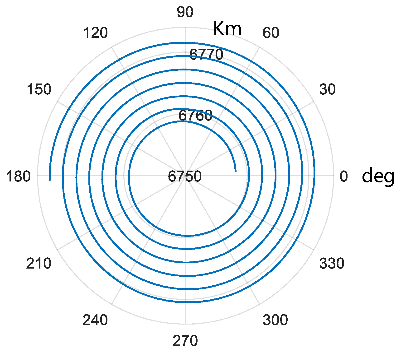
6. Simulation Analyses

We carried out simulation analyses of scenarios in which the number of satellite orbital elements is changed under continuous low thrust, given a satellite with an initial orbital altitude of 380 km and a continuous low thrust applied at 12:00 on 25 January 2024. The thrust parameters are set with reference to Starlink V2.0mini. The thruster specific impulse is 2500 s, the electric thrust magnitude is 170 mN, and the thrust acceleration is 2.26 × 10⁻⁴ m/s². The initial orbital elements of the satellite ignition point are shown in

Table 2. Initial orbital elements at the ignition point of a Starlink satellite.

Orbital Altitude/km	Eccentricity	Inclination/(°)	RAAN/(°)	Argument of Perigee/(°)	Mean Anomaly/(°)
380	0	53	352.937	336.98	63.025

, and other simulation parameters were set as in Table 1.

Assuming that radar equipment located at different locations can acquire satellite measurements, information on the distribution location of radar equipment is shown in

Table 3. Ground radar equipment latitude and longitude data.

Station Name	Fac1	Fac2	Fac3	Fac4	Fac5
Latitude	34.5869 N	46.82 N	38.83 N	36.06 N	18.2 N
Longitude	109.51 E	130.37 E	76.92 E	120.36 E	109.5 E
Station Name	Fac6	Fac7	Fac8	Fac9
Latitude	41.515 N	5.757 N	31.818 S	8.181 S
Longitude	14.362 E	44.059 E	22.543 E	38.062 W

. It is assumed that the radar distance measurement accuracy is 30 m (1σ), the angle measurement accuracy is 0.01° (1σ), and the minimum elevation angle is 5°. The simulation gives radar measurements of the satellite (azimuth, elevation, and range).

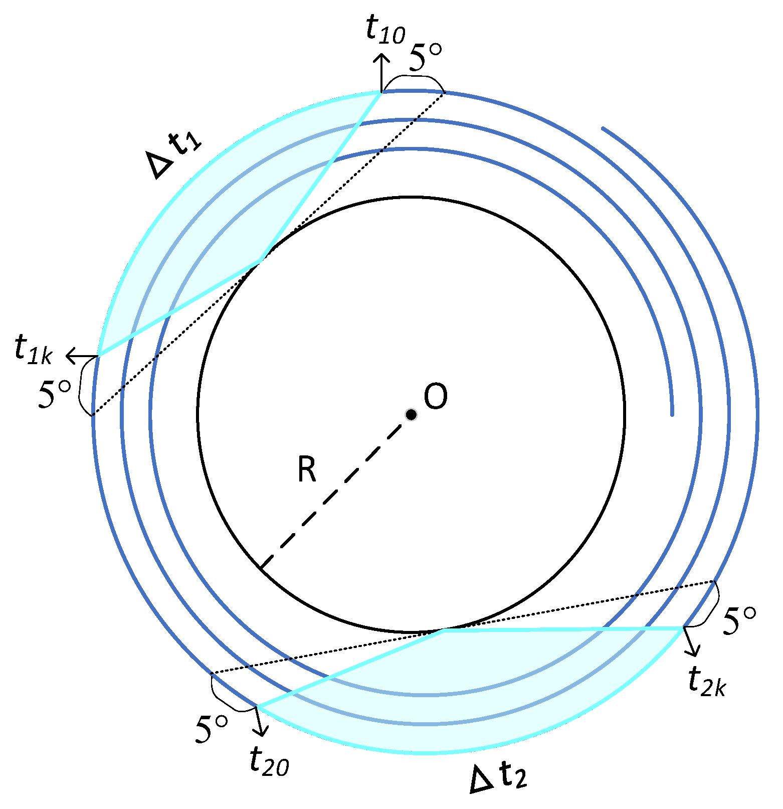
The thrust acceleration results are derived from the inverse solution of two radar observations separated by a certain length of time. Let the initial moments of the two radar observation arcs be $t_{10}$, $t_{20}$, and the ending moments be $t_{1k}$, $t_{2k}$, and the observation durations be $\Delta t_1$, $\Delta t_2$. The time intervals between them are denoted as Δt. The length of the visible arc segment at a single station varies from 3 to 9 min depending on the different positions of the satellite in relation to the station. In order to ensure the accuracy of the semi-major axis solution, only arc segments with observed arc segments greater than 6 min were selected for orbit determination.

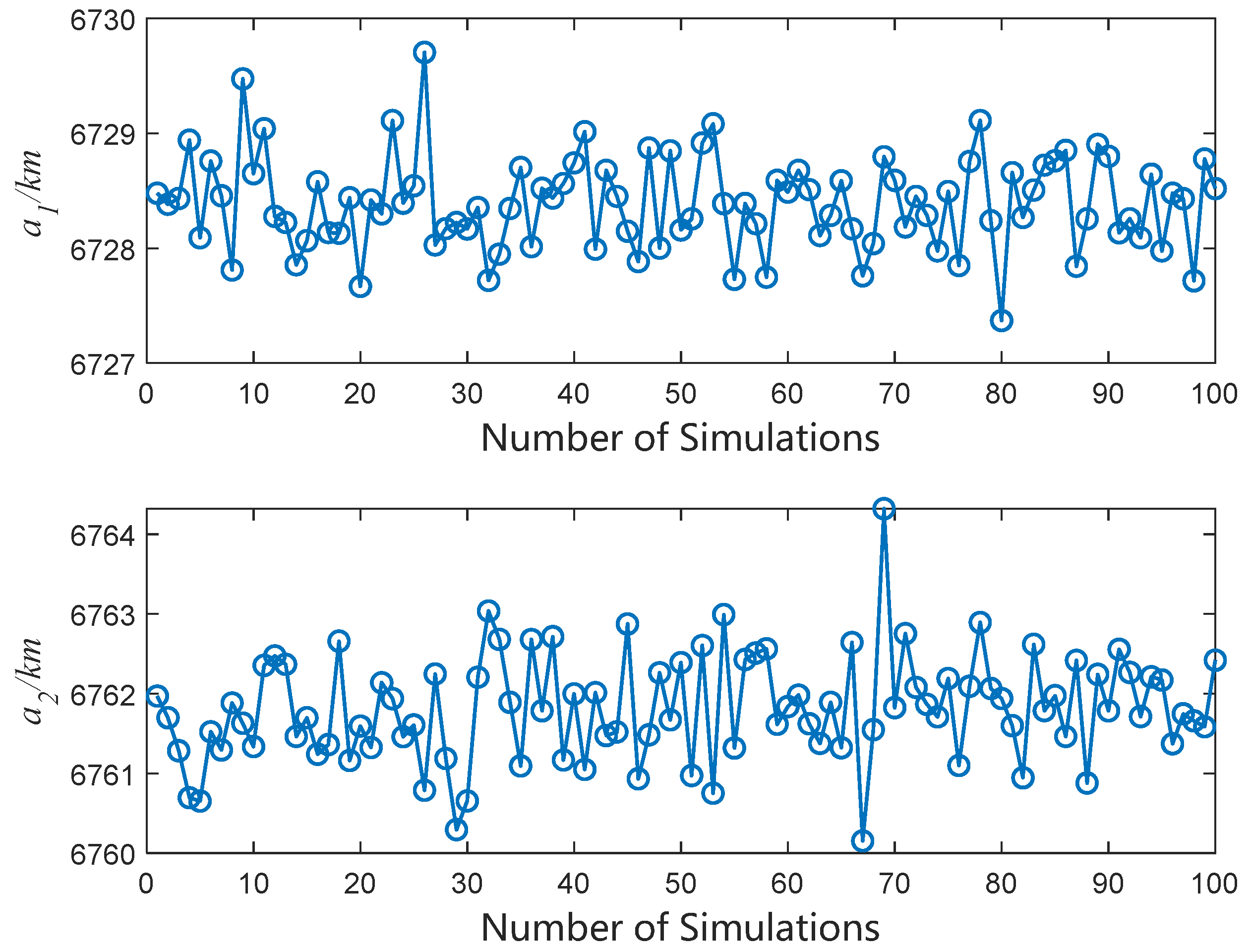
6.1. Pre-Identification of Continuous Tangential Thrust Parameters

Take, for example, the two observations described in

Table 4. Arc time for two observations.

$t_{10}$	$t_{1k}$	$\Delta t_1$
2024-01-25 12:05:01	2024-01-25 12:12:28	00:07:27
$t_{20}$	$t_{2k}$	$\Delta t_2$
2024-01-26 11:34:40	2024-01-26 11:43:15	00:08:25
$\Delta t$	23:29:39

.

The two observations were each simulated 100 times, and each simulation exhibited a different random observation error after using the single-arc segment orbit determination method described in Section 3 to obtain the semi-major axes of the two arc segments noted as $a_1$, $a_2$. The results are shown in Figure 8.

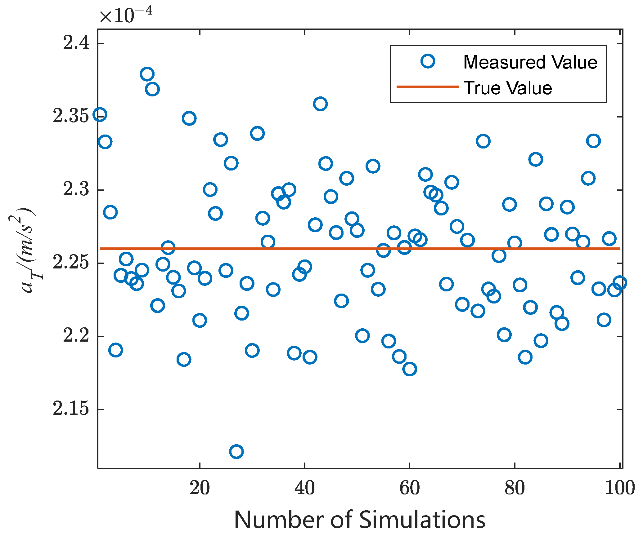
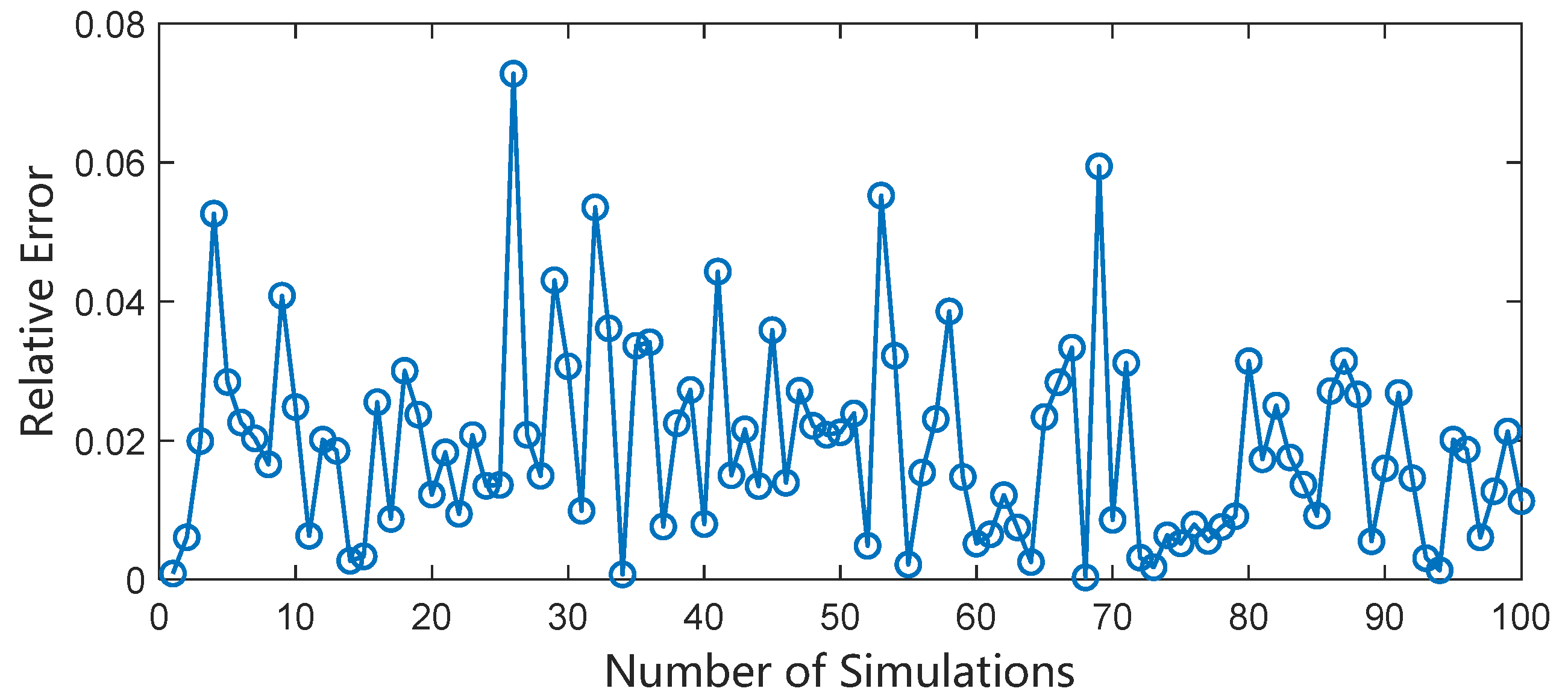
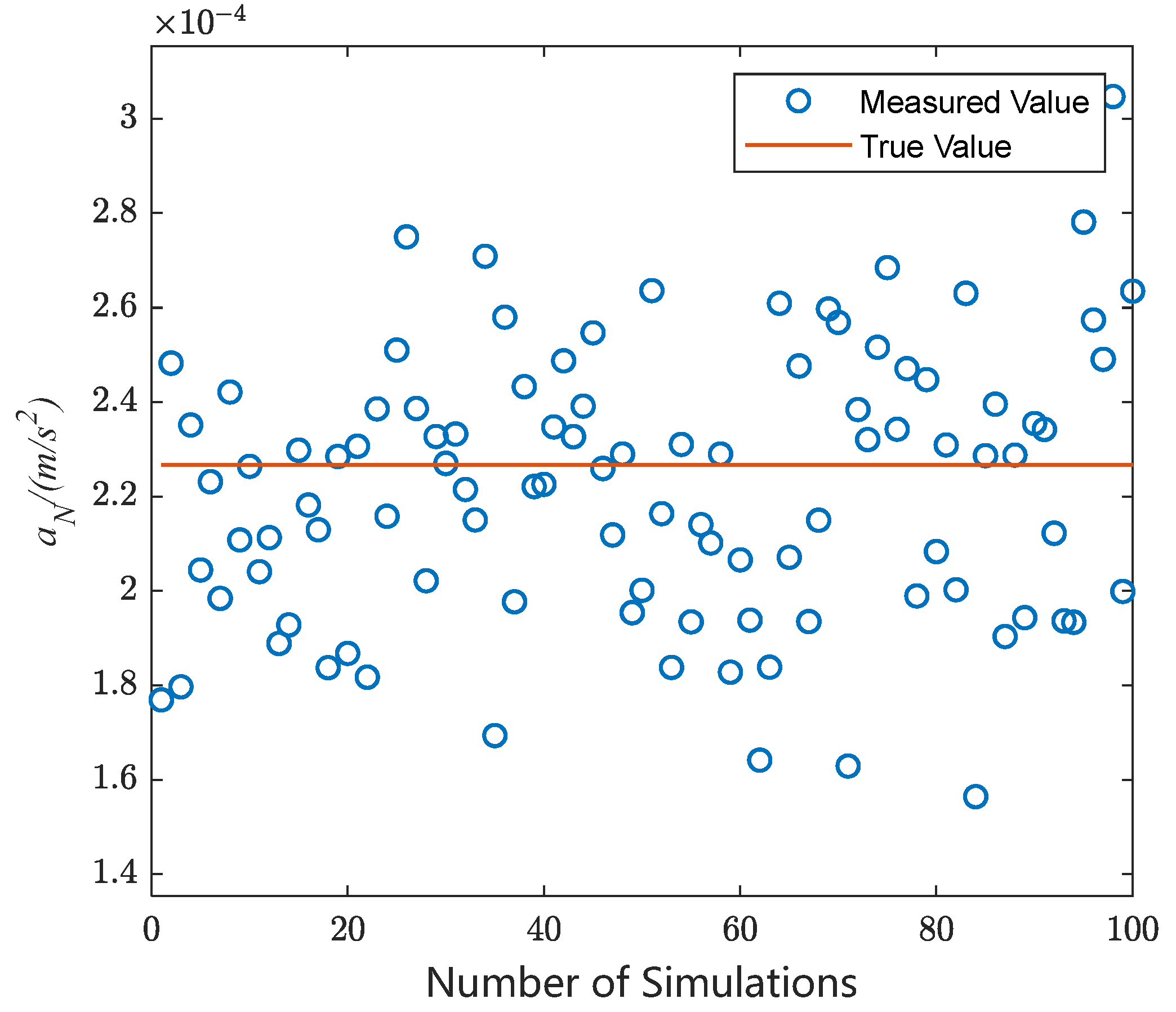
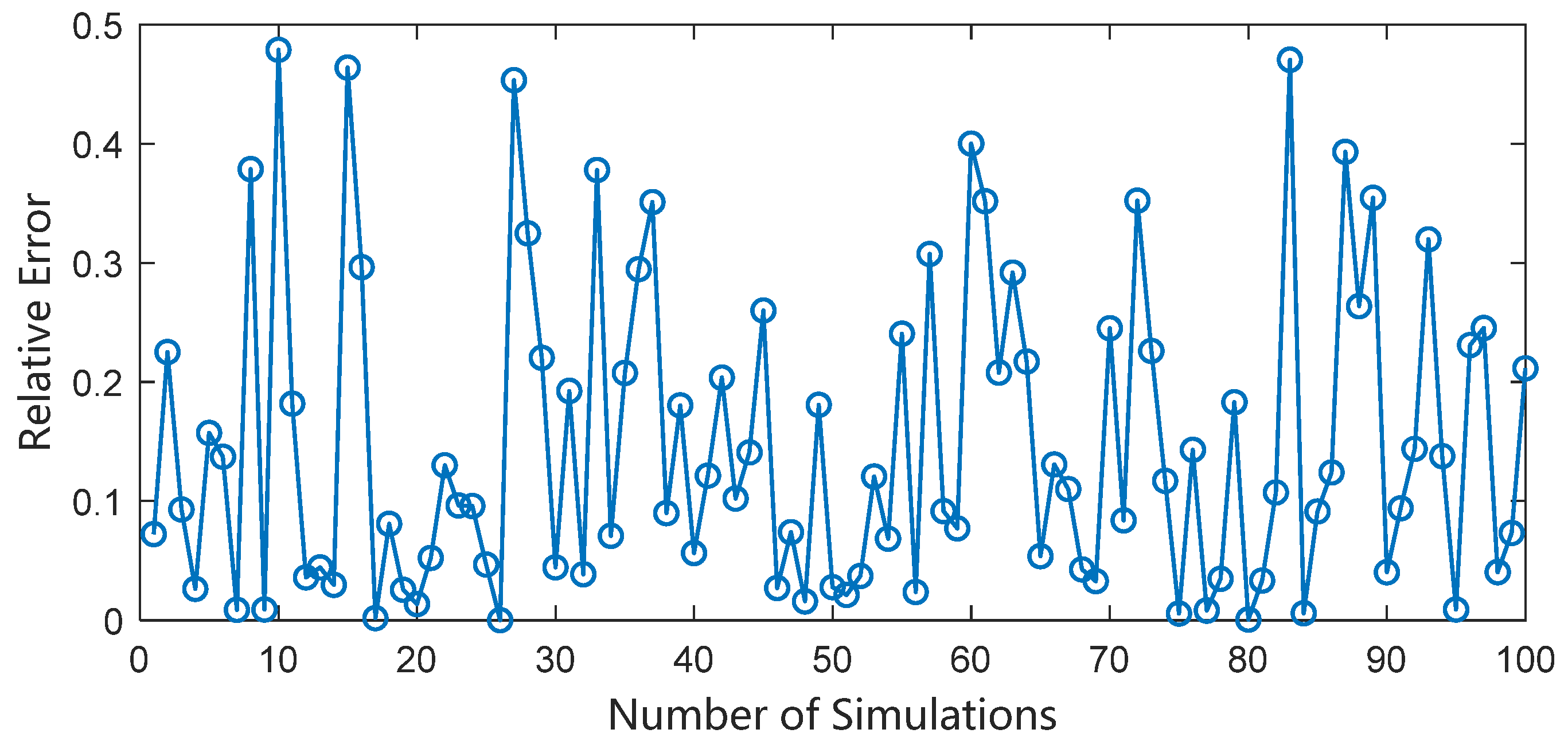
According to Equation (20), the tangential acceleration is solved inversely by $a_1$ and $a_2$. The results are shown in Figure 9, and the relative error of tangential acceleration is shown in Figure 10. It can be seen that the average relative error of solving the tangential acceleration based on two arc segments separated by 23 h is only 3.2%.

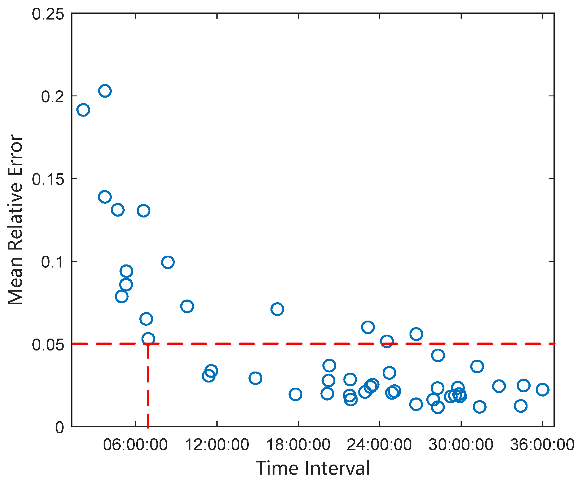
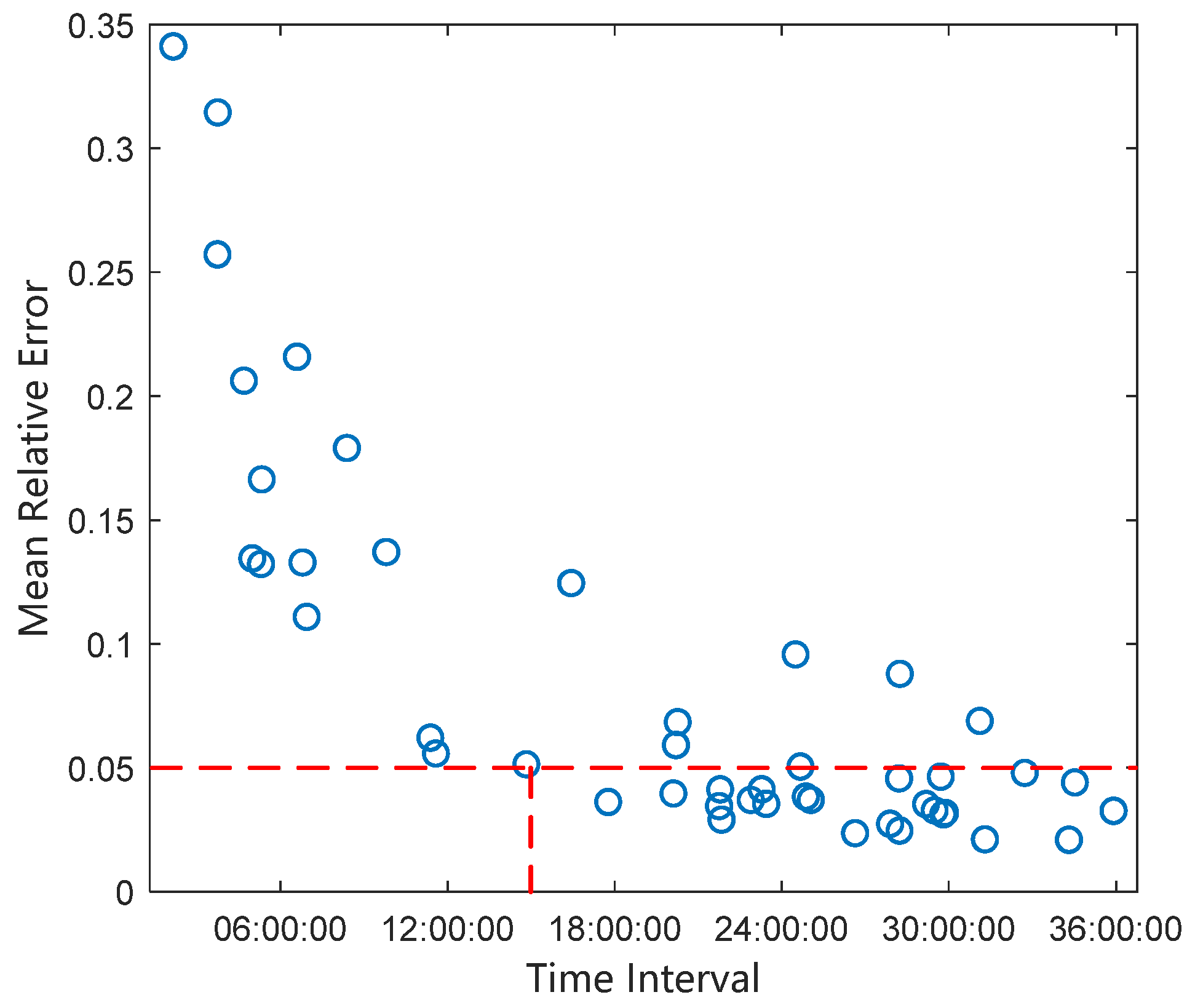
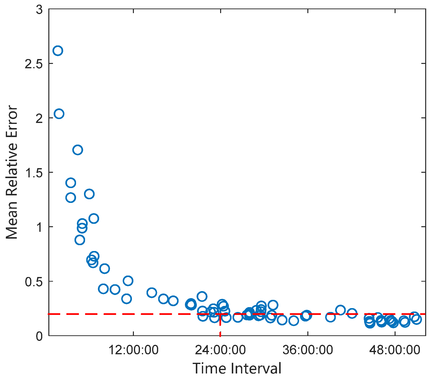
The tangential acceleration and its average relative error were calculated from radar observation arcs at different time intervals, and the relationship between the relative error of tangential acceleration and the observation time interval is shown. When the time interval between two observations is greater than 7 h, the relative measurement error of tangential acceleration can reach 5% or less. This is shown in Figure 11. The circles in the figure represent the average relative error values of 100 observations at that moment.

Electric propellers usually have multi-mode operation capability, and their performance in terms of thrust, power, and specific impulse can be optimally adjusted according to different mission requirements, with strong mission adaptability. The smaller the tangential acceleration, the slower the rate of change of the semi-major axis and, consequently, the poorer the accuracy of the tangential acceleration inversely solved from the orbit determination of the two radar observations. A longer interval between two radar observations is required to achieve a relative measurement error of 5%.

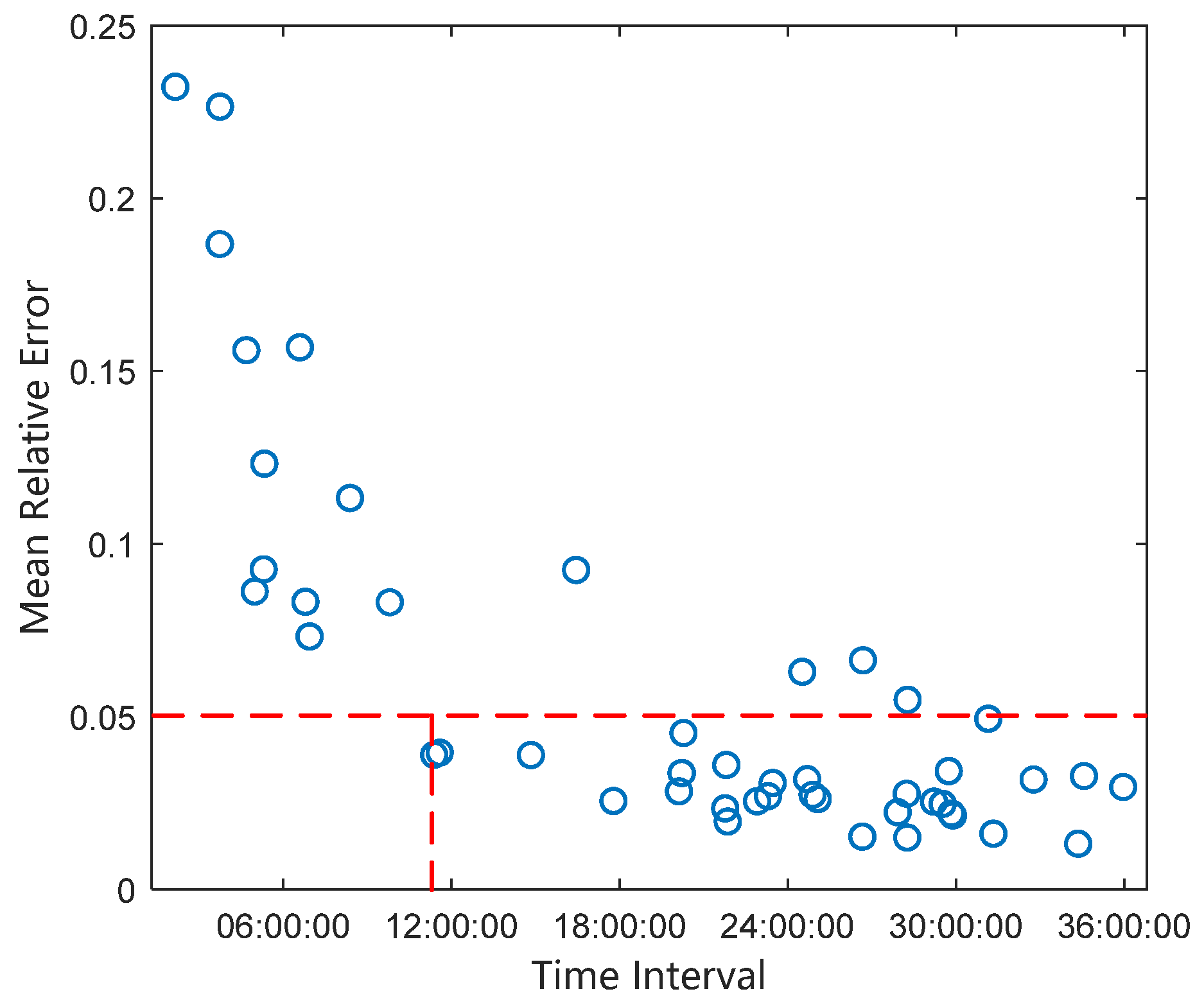
The simulation is set up with continuous tangential accelerations of 1.8 × 10⁻⁴ m/s², 1.3 × 10⁻⁴ m/s² and 0.5 × 10⁻⁴ m/s². The results are shown in Figure 12, Figure 13, and Figure 14, respectively.

When the continuous tangential acceleration is 1.8 × 10⁻⁴ m/s² and the interval between two radar observations is greater than 11 h, a solution error of 5% or less can be achieved. When the continuous tangential acceleration is 1.3 × 10⁻⁴ m/s² and the interval between two radar observations is greater than 15 h, a solution error of 5% or less can be achieved. When the continuous low-thrust acceleration is 0.5 × 10⁻⁴ m/s², the change in track elements caused by thrust is too small, the error of thrust parameter identification is large in the short cycle, and the pre-identification of tangential acceleration below 5% cannot be achieved within 24 h.

6.2. Pre-Identification of Continuous Normal Thrust Parameters for Changing Inclinations

Take, for example, the two observations described in

Table 5. Arc time for two observations.

$t_{10}$	$t_{1k}$	$\Delta t_1$
25 January 2024 12:08:21	25 January 2024 12:16:12	00:07:51
$t_{20}$	$t_{2k}$	$\Delta t_2$
26 January 2024 11:09:01	26 January 2024 11:15:42	00:06:41
$\Delta t$	23:00:40

.

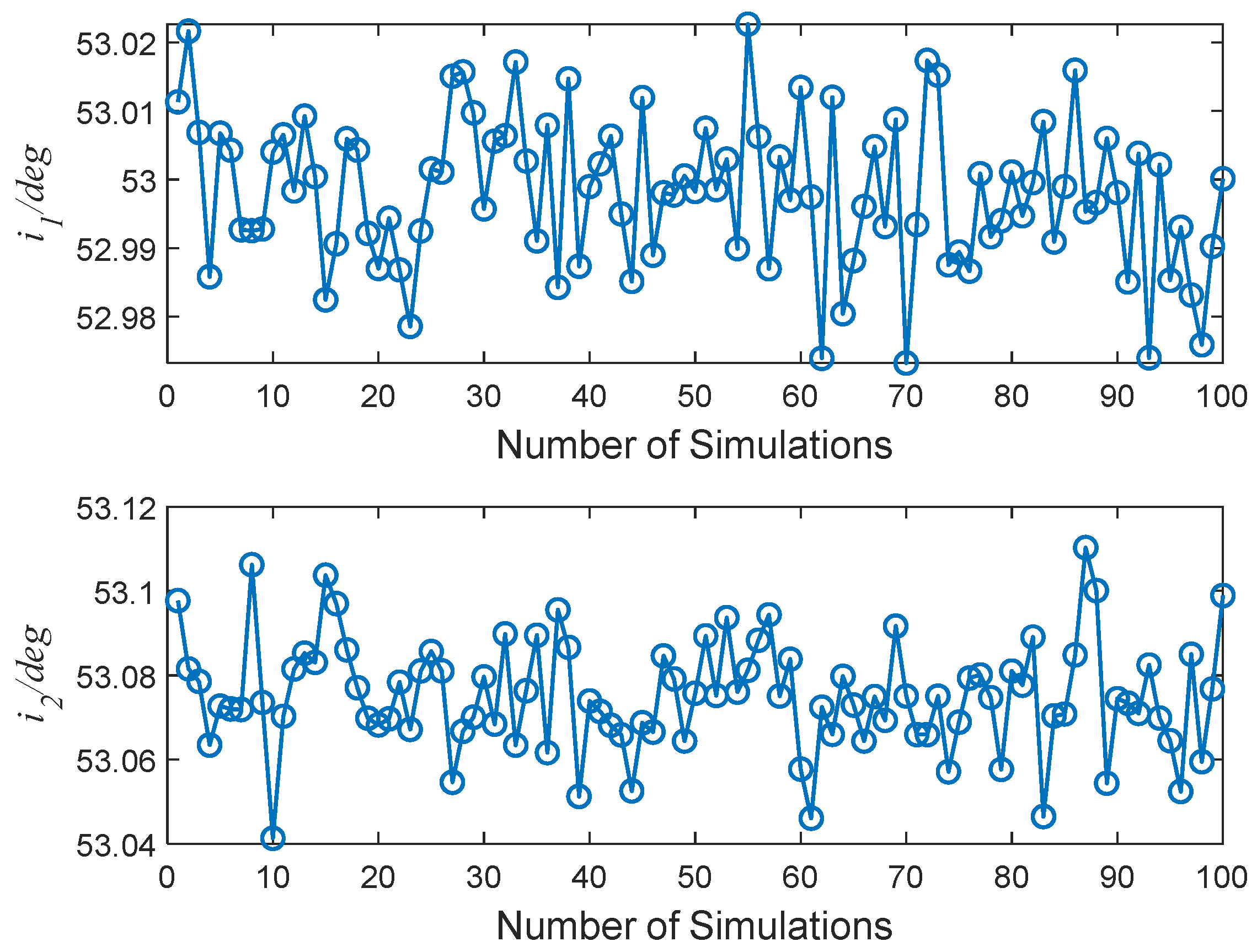
The two observations are simulated 100 times, and each simulation exhibits a different random observation error when using the single-arc segment orbit determination method described in Section 3 to obtain the orbit inclination of the two arc segments noted as $i_1$, $i_2$. The results are shown in Figure 15.

According to Equation (26), the normal acceleration is solved inversely by $i_1$ and $i_2$; the result is shown in Figure 16. The relative error in normal acceleration is shown in Figure 17. It can be seen that solving for the normal acceleration based on two arcs separated by 23 h gives an average relative error of 21.5%.

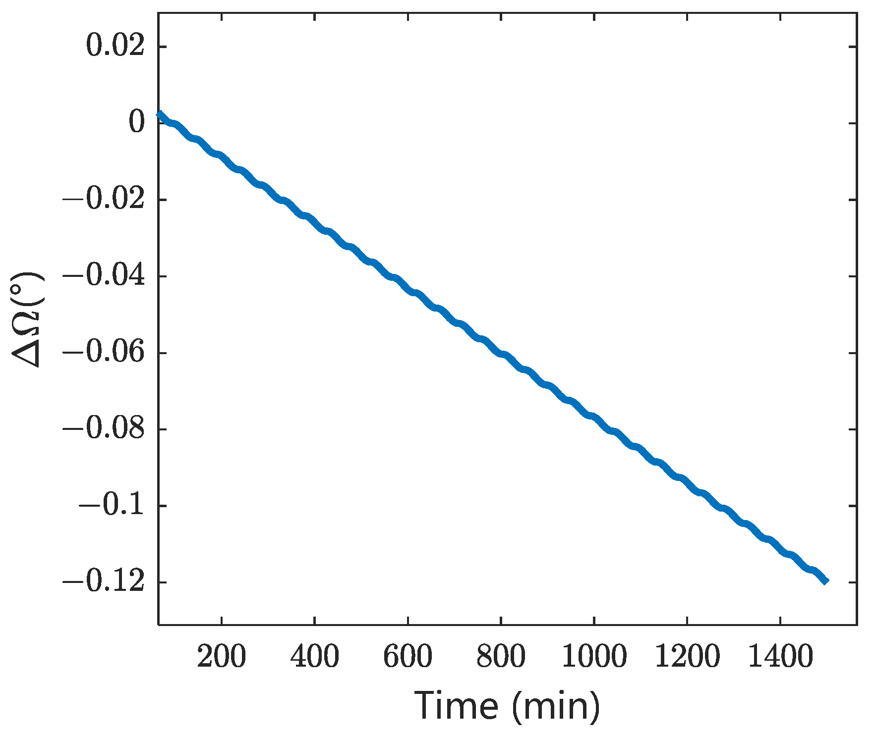
6.3. Pre-Identification of Continuous Normal Thrust Parameters for Changing RAAN

Take, for example, the two observations described in

Table 6. Arc time for two observations.

$t_{10}$	$t_{1k}$	$\Delta t_1$
25 January 2024 12:08:21	25 January 2024 12:16:12	00:07:51
$t_{20}$	$t_{2k}$	$\Delta t_2$
26 January 2024 11:14:23	26 January 2024 11:20:33	00:06:10
$\Delta t$	23:06:02

.

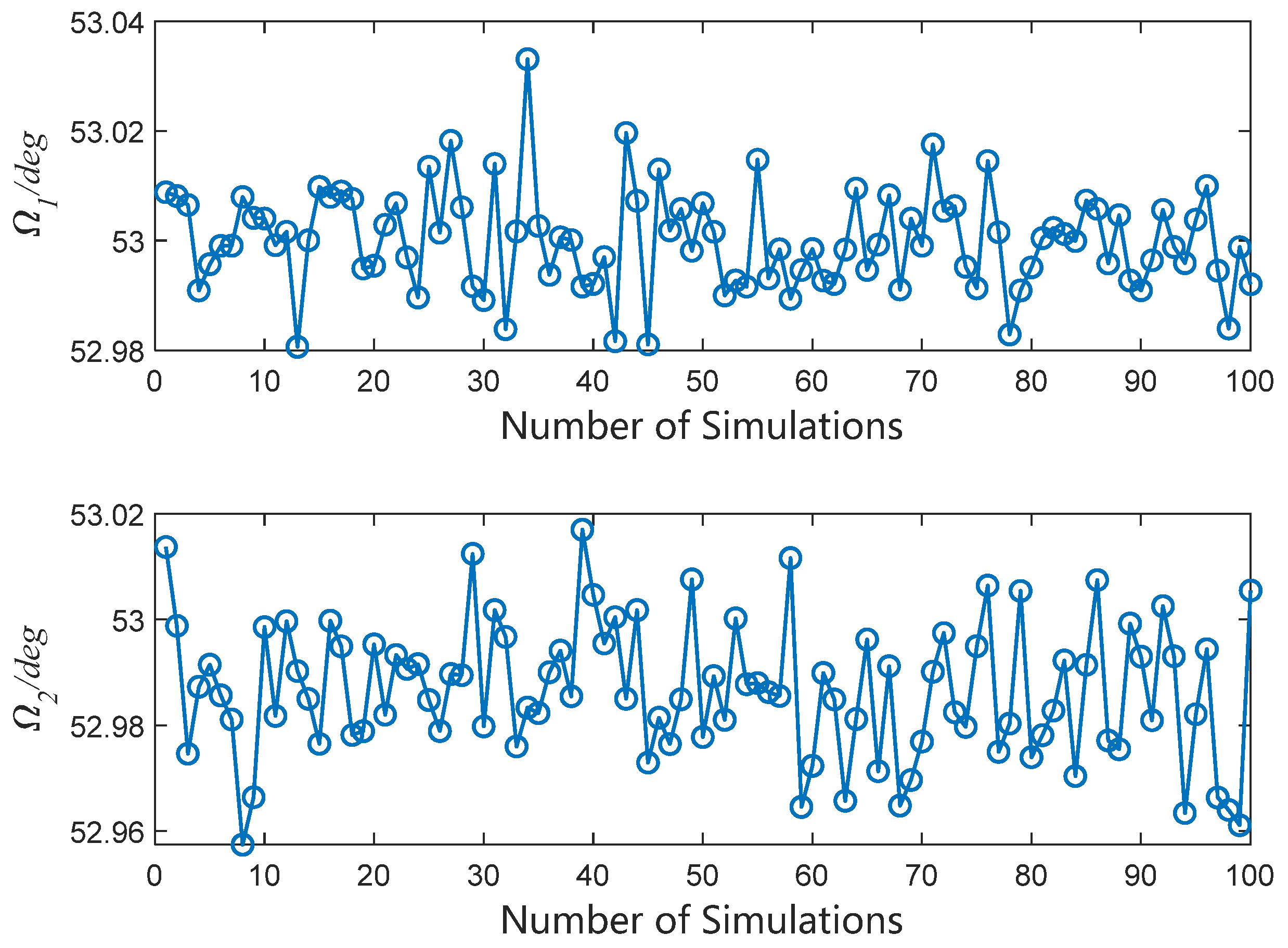
The two observations were each simulated 100 times. Each simulation imposes a different random observation error using the single-arc segment orbit determination method described in Section 3 to obtain the RAAN of the two arcs noted as ${\Omega }_1$, ${\Omega }_2$. The results are shown in Figure 18.

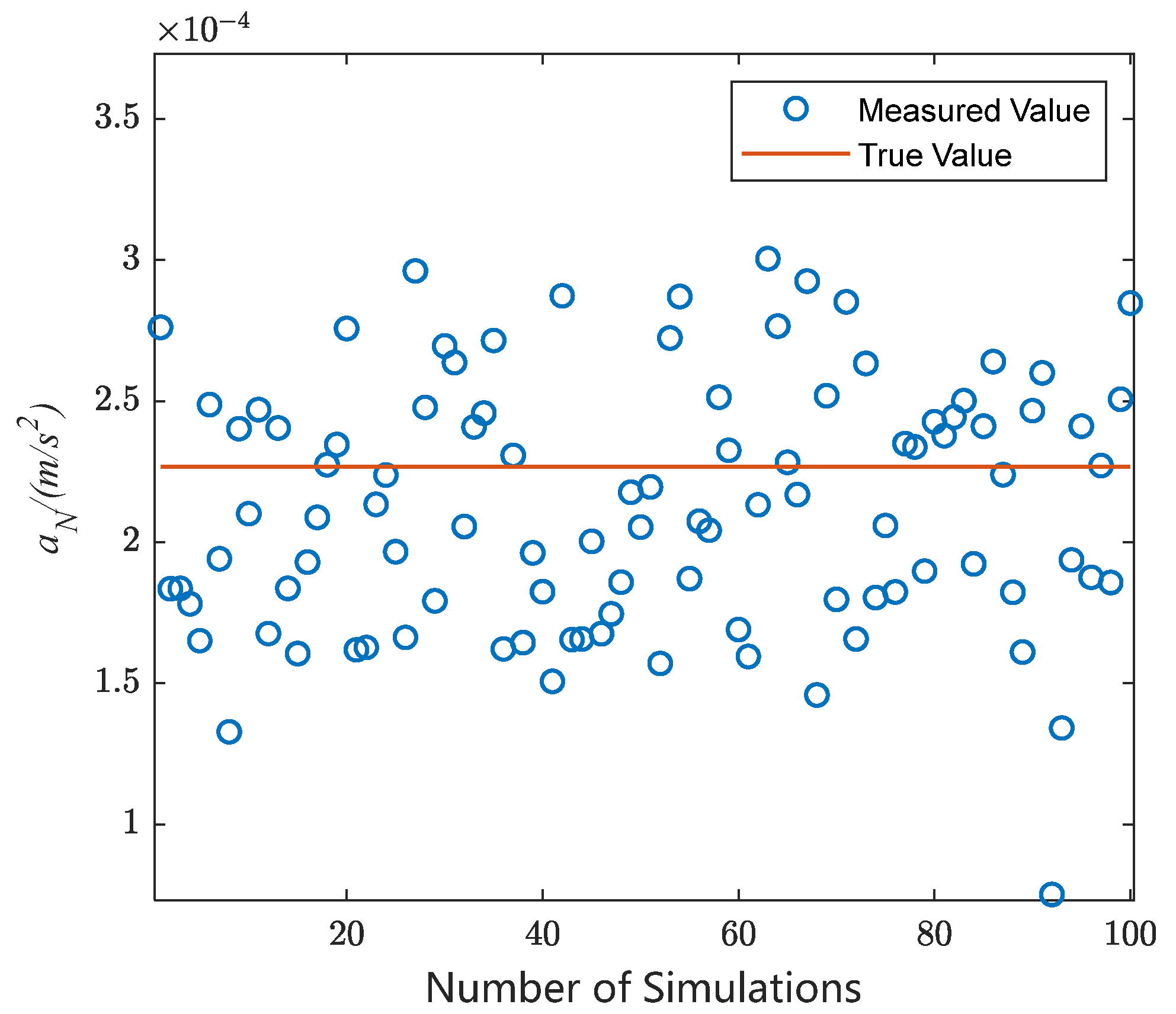
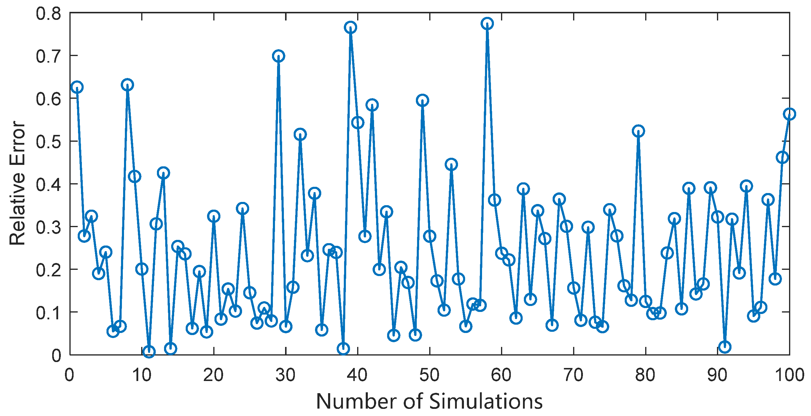
According to Equation (30), the normal acceleration is solved inversely by ${\Omega }_1$ and ${\Omega }_2$. The results are shown in Figure 19. The relative error in normal acceleration is shown in Figure 20. It can be seen that solving for the normal acceleration based on two arcs separated by 23 h gives an average relative error of 30.21%.

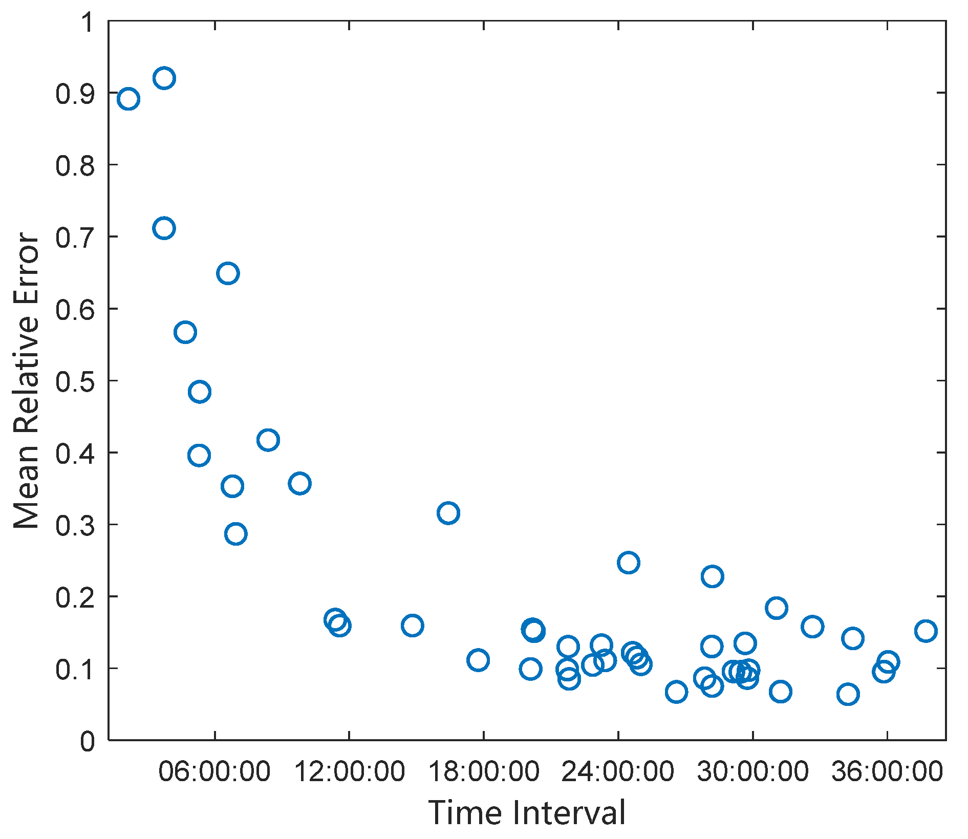
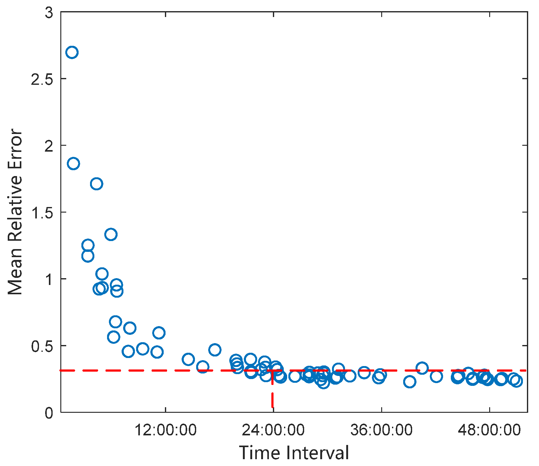
The normal acceleration and its average relative error are calculated separately from radar observation arcs at different time intervals. The relative error of the normal acceleration versus the observation interval is shown in Figure 21. The observation angle error of the radar equipment is large, so the relative error will also be larger compared to the tangential acceleration determined via orbit determination using radar observation data and inverting the normal acceleration. The average relative measurement error of normal acceleration is about 20% when the interval between observations is 24 h.

Depending on the mission requirements, the smaller the normal acceleration, the smaller the rate of change of orbital inclination and RAAN. When the continuous normal acceleration is reduced to 1.4 × 10⁻⁴ m/s², the average relative measurement error of the normal acceleration can only be about 35% when the time interval between two observations is 24 h. This is shown in Figure 22.

6.4. The Relationship Between Orbit Determination Accuracy and Measurement Accuracy

The measurement data obtained by the radar measurement equipment are the azimuth angle A, elevation angle E, and range ρ. There are many factors that affect measurement accuracy, among which atmospheric disturbances and irregularities in the ionosphere are important factors.

Atmospheric refraction causes radio waves to bend, resulting in the apparent distance and elevation angle measured by radar differing from the actual distance and elevation angle. To address the errors in radar ranging and angle measurement caused by atmospheric refraction, researchers have focused their efforts on two main areas: first, studying how to obtain atmospheric refraction indices that more closely match actual conditions [19,20]; second, proposing more accurate and efficient models and correction methods for radio wave refraction errors [21,22].

The accuracy of measurement data affects the accuracy of precise orbit determination and thrust parameter estimation. Taking the pre-identification process of tangential thrust parameters as an example, we will analyze the impact of angular measurement and range measurement accuracy on the accuracy of thrust parameter pre-identification.

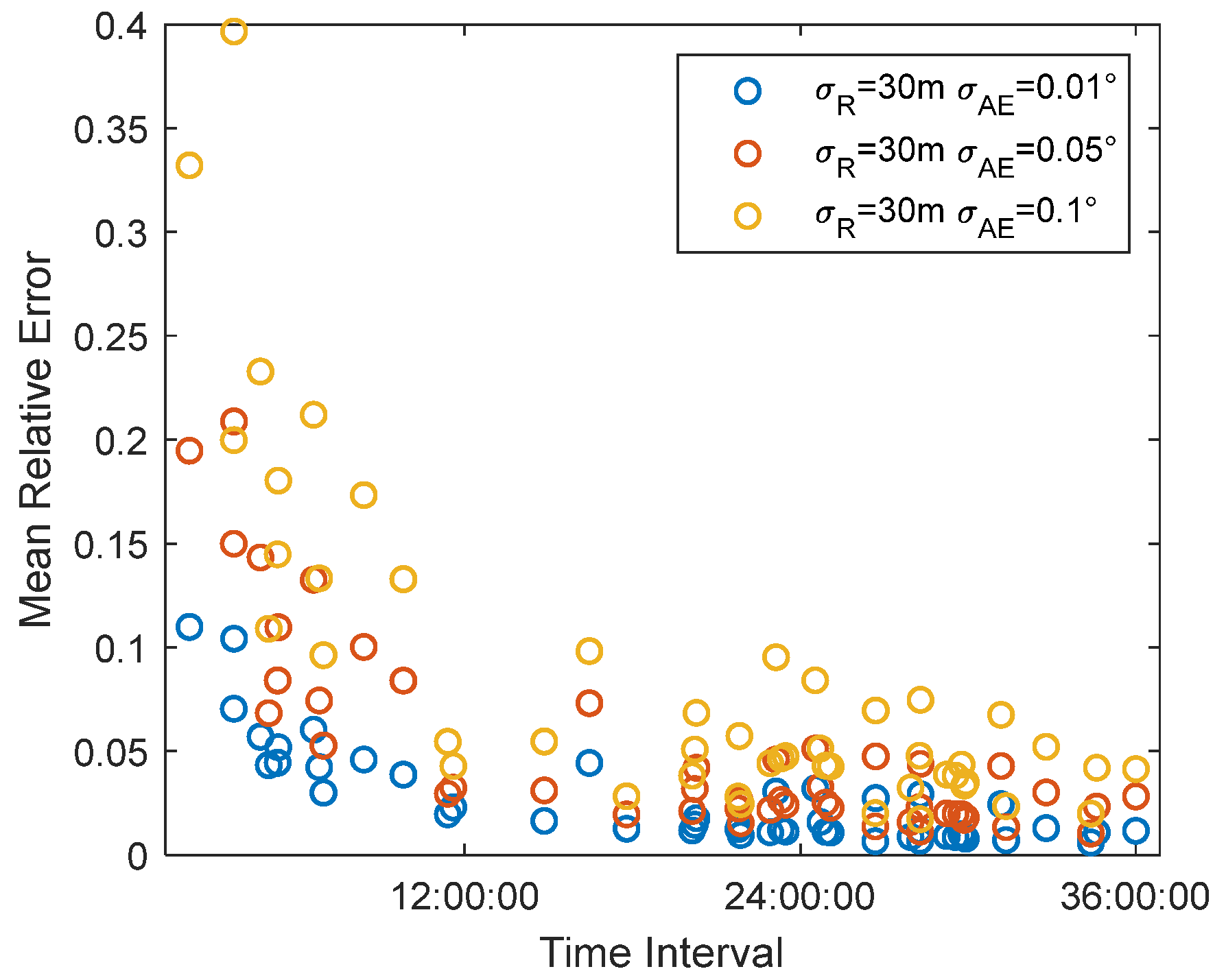
6.4.1. The Effect of Angle Measurement Accuracy on Orbit Determination Accuracy

When the range measurement accuracy is 30 m, the angle measurement accuracy is set to 0.01°, 0.05°, and 0.1°. The relationship between the thrust parameter pre-identification accuracy and the time span is shown in the Figure 23.

As the angular measurement accuracy decreases, the average relative error of the thrust parameter pre-identification also decreases. When the angular measurement accuracy is 0.01°, a 5% solution error can be achieved within 4 h; when the angular measurement accuracy is 0.05°, a 5% solution error can be achieved within 8 h; when the angular measurement accuracy is 0.1°, a 5% solution error can be achieved within 12 h.

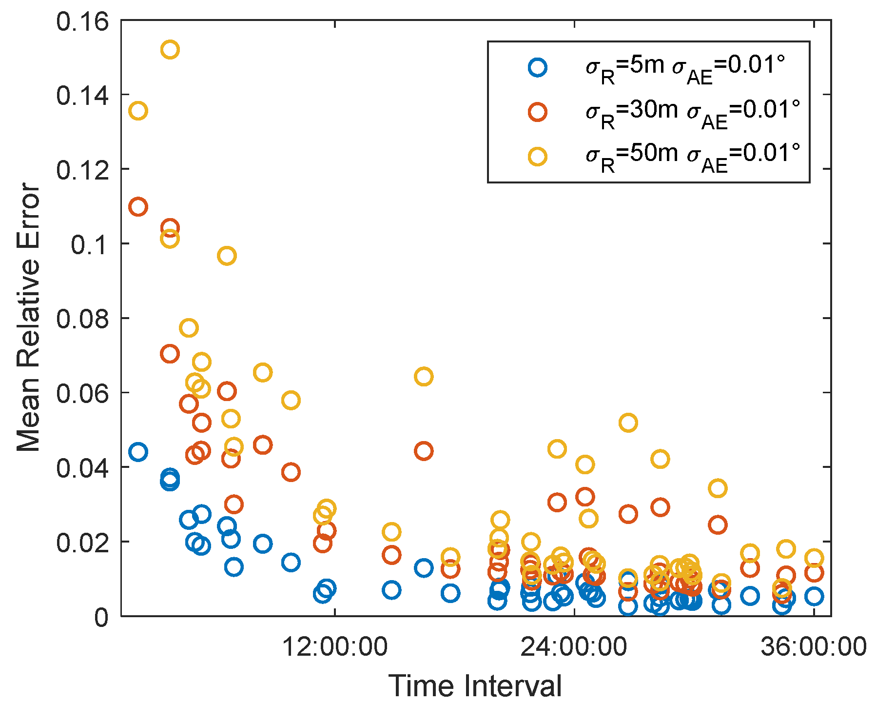
6.4.2. The Effect of Range Measurement Accuracy on Orbit Determination Accuracy

When the angle measurement accuracy is 0.01°, the range measurement accuracy is set to 5 m, 30 m, and 50 m. The relationship between the thrust parameter pre-identification accuracy and the time span is shown in the Figure 24.

As the ranging accuracy decreases, the average relative error of thrust parameter pre-identification also decreases. When the ranging accuracy is 5 m, a 5% solution error can be achieved within 2 h; when the ranging accuracy is 30 m, a 5% solution error can be achieved within 6 h; when the ranging accuracy is 50 m, a 5% solution error can be achieved within 8 h.

Both angular measurement and range measurement accuracy affect the accuracy of thrust parameter pre-identification, and the degree of impact is basically the same. When angular measurement or range measurement accuracy decreases by a factor of 10, the average relative error of thrust parameter pre-identification increases by about 8 times.

7. Conclusions

In this paper, a rapid method for pre-identifying tangential acceleration based on ground radar observation is proposed for the problem of identifying the maneuvering parameters of non-cooperative space targets. A dynamic model of a satellite under continuous low thrust is given that can derive the relationship between the change in satellite orbital elements and the direction and magnitude of acceleration during continuous thrust control. We can pre-determine continuous acceleration using a single-arc segment orbit determination method based on the least-squares approach. Initial values of orbital elements and thrust parameters can be used for precision orbit determination to improve its accuracy and efficiency. However, in our study, we did not consider changes in the mass of the electric propulsion system. This is because we assumed that changes in propellant mass could be ignored and neglected its effect on acceleration. In future studies, we will adjust our research assumptions to improve the practical value of the experiment.

References

1. Hussain, K.F.; Safwat, N.E.-D.; Thangavel, K.; Sabatini, R. Space-based debris trajectory estimation using vision sensors and track-based data fusion techniques. Acta Astronaut. 2025, 229, 814–830. [Google Scholar] [CrossRef]
2. Lyu, Y.; Wang, C.; Li, X.; Zheng, Z.; Guo, Y. Improved particle swarm orbit-keeping optimization design for GEO satellite with electric propulsion. J. Astronaut. 2024, 45, 523–531. [Google Scholar]
3. Wu, C.; Hai, G.; Wang, Z.; Li, D. Development of advanced electric propulsion technology for cislunar and deep space exploration. Chin. Space Sci. Technol. 2023, 43, 13–23. [Google Scholar]
4. Yeo, S.H.; Ogawa, H.; Kahnfeld, D.; Schneider, R. Miniaturization perspectives of electrostatic propulsion for small spacecraft platforms. Prog. Aerosp. Sci. 2021, 126, 100742. [Google Scholar] [CrossRef]
5. Lenz, S.M.; Bock, H.G.; Schlöder, J.P.; Kostina, E.A.; Gienger, G.; Ziegler, G. Multiple shooting method for initial satellite orbit determination. J. Guid. Control Dynam. 2012, 33, 1334–1346. [Google Scholar] [CrossRef]
6. Ansalone, L.; Curti, F. A genetic algorithm for Initial Orbit Determination from a too short arc optical observation. Adv. Space Res. 2013, 52, 477–489. [Google Scholar] [CrossRef]
7. Scir’e, G.; Santoni, F.; Piergentili, F. Analysis of orbit determination for space based optical space surveillance system. Adv. Space Res. 2015, 56, 421–428. [Google Scholar] [CrossRef]
8. Goff, G.M.; Black, J.T.; Beck, J.A. Tracking maneuvering spacecraft with filter-through approaches using interacting multiple models. Acta Astronaut. 2015, 114, 152–163. [Google Scholar] [CrossRef]
9. Flohrer, T.; Krag, H.; Klinkrad, H.; Schildknecht, T. Feasibility of performing space surveillance tasks with a proposed space-based optical architecture. Adv. Space Res. 2011, 47, 1029–1042. [Google Scholar] [CrossRef]
10. Zhou, X.; Qin, T.; Ji, M.; Qiao, D. A LSTM assisted orbit determination algorithm for spacecraft executing continuous maneuver. Acta Astronaut. 2023, 204, 568–582. [Google Scholar] [CrossRef]
11. Escribano, G.; Sanjurjo-Rivo, M.; Siminski, J.A.; Pastor, A.; Escobar, D. A filter for tracking non-cooperative low-thrust satellites using surveillance radar data. Acta Astronaut. 2023, 213, 694–707. [Google Scholar] [CrossRef]
12. Zhang, J.; Zhu, T.; Zhao, C. Orbit determination for spacecraft with continuous low-thrust using nonsingular Thrust-Fourier-Coefficients and filtering-through approach. Acta Astronaut. 2024, 224, 353–366. [Google Scholar] [CrossRef]
13. Yu, S.; Wang, X.; Zhu, T. Maneuver detection methods for space objects based on dynamical model. Adv. Space Res. 2021, 68, 71–84. [Google Scholar] [CrossRef]
14. Zhou, X.; Dong, Q.; Macdonald, M. Orbit Determination for Impulsively Maneuvering Spacecraft Using Modified State Transition Tensor. J. Guid. Control Dynam 2024, 47, 822–839. [Google Scholar] [CrossRef]
15. Goff, M.G.; Showalter, D.; Black, T.J.; Beck, J.A. Parameter Requirements for Noncooperative Satellite Maneuver Reconstruction Using Adaptive Filters. J. Guid. Control Dyn. 2015, 38, 361–374. [Google Scholar] [CrossRef]
16. Li, H.; Li, J.; Huang, Y. On-line orbit determinative method for satellites with continuous thrust acceleration. Syst. Eng. Electron. 2010, 32, 1957–1961. [Google Scholar]
17. Liu, L.; Wang, J. On initial orbit determination. J. Spacecr. TT&C Technol. 2004, 23, 41–45, 50. [Google Scholar]
18. Xie, Y.; Lei, Y.; Guo, J. Spacecraft Dynamics and Control; Beijing Institute Technology Press: Beijing, China, 2018; pp. 132–133. [Google Scholar]
19. Tang, X.; Liu, M.; Qiao, J. Atmospheric refraction technology for space target surveillance radar. Chin. J. Radio Sci. 2024, 39, 148–155. [Google Scholar]
20. Li, C.; Liu, K.; Zhu, Q. Method of high-precision refraction error correction in S-band radar detection. J. Air Space Early Warn. Res. 2019, 33, 405–408. [Google Scholar]
21. Hang, W.; Zhang, X. Analytical formulae of radar location for measured atmospheric model with discussion on effective earth radius. J. Electron. Inf. Technol. 2005, 27, 269–273. [Google Scholar]
22. Wang, Z.; Ji, Y.; Dong, Z. Atmospheric refraction error correction approach for ground-based space-target surveillance radar. Chin. J. Radio Sci. 2024, 39, 570–578. [Google Scholar]
Figure 1. Variation in semi-major axis under the effect of tangential acceleration.
Applsci 15 08064 g001
Figure 2. Variation in eccentricity under the effect of tangential acceleration.
Applsci 15 08064 g002
Figure 3. Variation in argument of latitude under the effect of tangential acceleration.
Applsci 15 08064 g003
Figure 4. Variation in orbit inclination under normal thrust.
Applsci 15 08064 g004
Figure 5. Variation in RAAN under normal thrust.
Applsci 15 08064 g005
Figure 6. Schematic of the two observation arcs.
Applsci 15 08064 g006
Figure 7. Flowchart of the continuous low thrust parameter pre-identification method.
Applsci 15 08064 g007
Figure 8. Semi-major axis results for two initial orbit determinations.
Applsci 15 08064 g008
Figure 9. Results of tangential acceleration calculation.
Applsci 15 08064 g009
Figure 10. Relative error of tangential acceleration.
Applsci 15 08064 g010
Figure 11. Mean relative error versus observation interval for an acceleration of 2.26 × 10⁻⁴ m/s2.
Applsci 15 08064 g011
Figure 12. Mean relative error versus observation interval for an acceleration of 1.80 × 10⁻⁴ m/s2.
Applsci 15 08064 g012
Figure 13. Mean relative error versus observation interval for an acceleration of 1.30 × 10⁻⁴ m/s2.
Applsci 15 08064 g013
Figure 14. Mean relative error versus observation interval for an acceleration of 0.5 × 10⁻⁴ m/s2.
Applsci 15 08064 g014
Figure 15. Semi-major axis results for two initial orbit determinations.
Applsci 15 08064 g015
Figure 16. Calculated normal acceleration for changing inclination.
Applsci 15 08064 g016
Figure 17. Relative error in normal acceleration for changing the inclination of orbit.
Applsci 15 08064 g017
Figure 18. RAAN results for two initial orbit determinations.
Applsci 15 08064 g018
Figure 19. Calculated normal acceleration for changing RAAN.
Applsci 15 08064 g019
Figure 20. Relative error in normal acceleration for changing the RAAN of the orbit.
Applsci 15 08064 g020
Figure 21. Mean relative error of normal acceleration solution versus time interval for an acceleration of 2.26 × 10⁻⁴ m/s2.
Applsci 15 08064 g021
Figure 22. Mean relative error of normal acceleration solution versus time interval for an acceleration of 1.40 × 10⁻⁴ m/s2.
Applsci 15 08064 g022
Figure 23. Relationship between average relative error and time interval in acceleration identification at different angle measurement accuracies.
Applsci 15 08064 g023
Figure 24. Relationship between average relative error and time interval in acceleration identification at different range measurement accuracies.
Applsci 15 08064 g024