

AI-Based Damage Risk Prediction Model Development Using Urban Heat Transport Pipeline Attribute Information


Abstract
1. Introduction
2. Research Method and Data
2.1. Research Method
2.2. Heat Transport Pipeline Data
2.2.1. Data Types
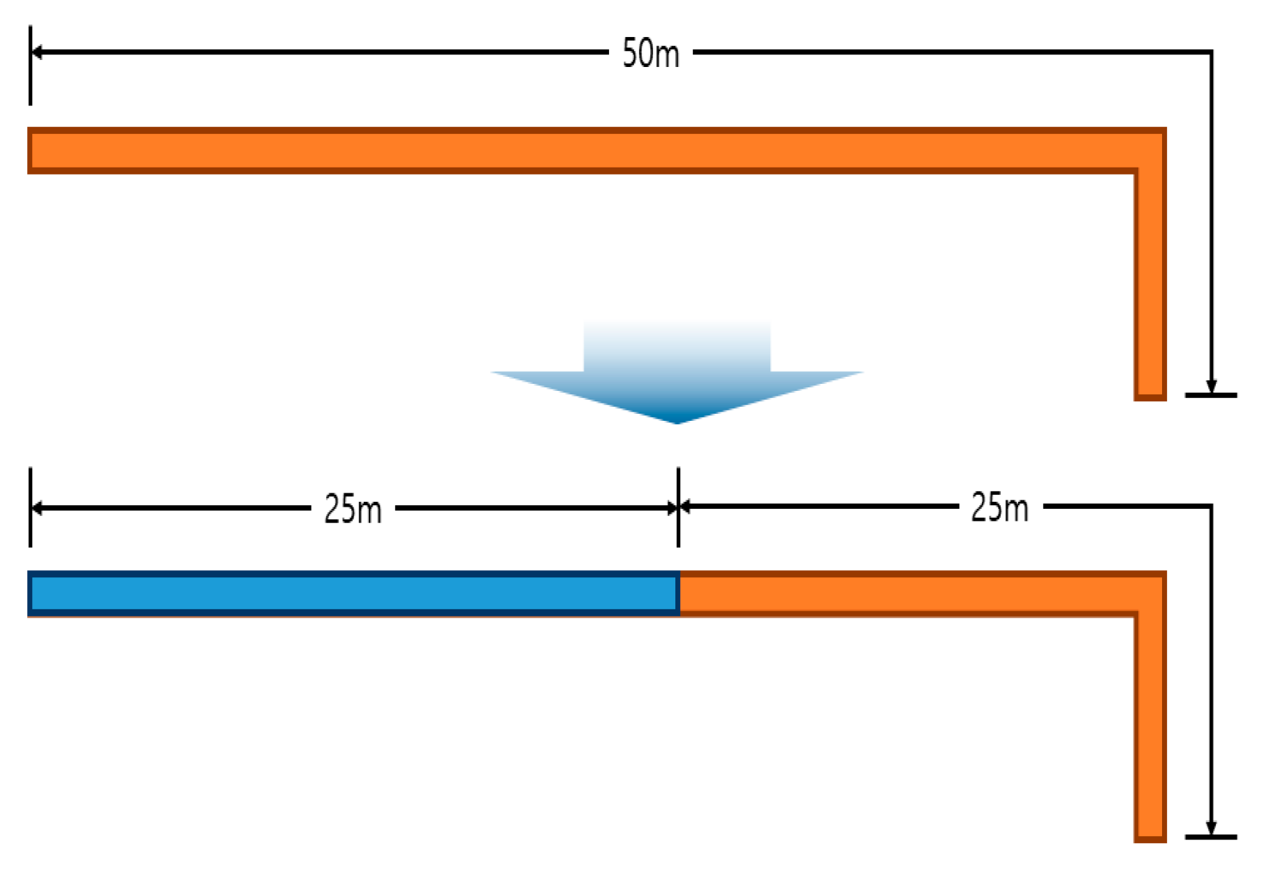
2.2.2. Basic Unit Setting
Combination of Heat Transport Pipelines Based on Attribute Information
Maximum and Minimum Length Setting
2.2.3. Damage History Data
3. Heat Transport Pipeline Damage Probability Analysis
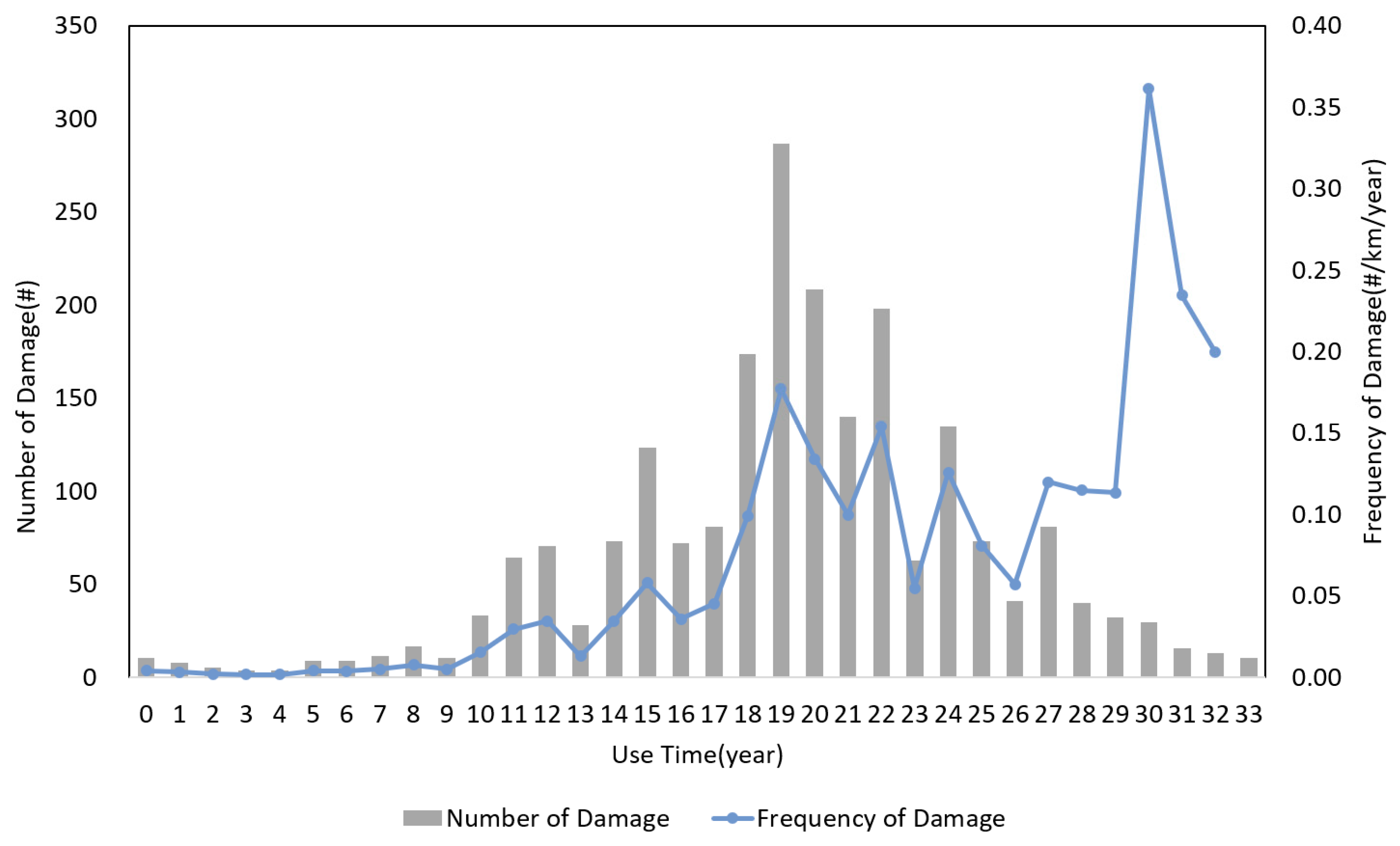
3.1. Period of Use
- ›
- : Number of damage cases for heat transport pipelines used for Yu years (#) (corrected value).
- ›
- : Number of damage cases for heat transport pipelines used for Yu years (#) (actual value).
- ›
- : Number of damage cases with period-of-use information (1761).
- ›
- : Number of damage cases without period-of-use information (504).
- ›
- : Damage probability according to the period of use (#/km/year).
- ›
- : Number of heat transport pipeline damage cases by period of use (#).
- ›
- : Length of heat transport pipelines by period of use (km).
- ›
- : Relevant year (year).
- ›
- : Damage history collection period (year).
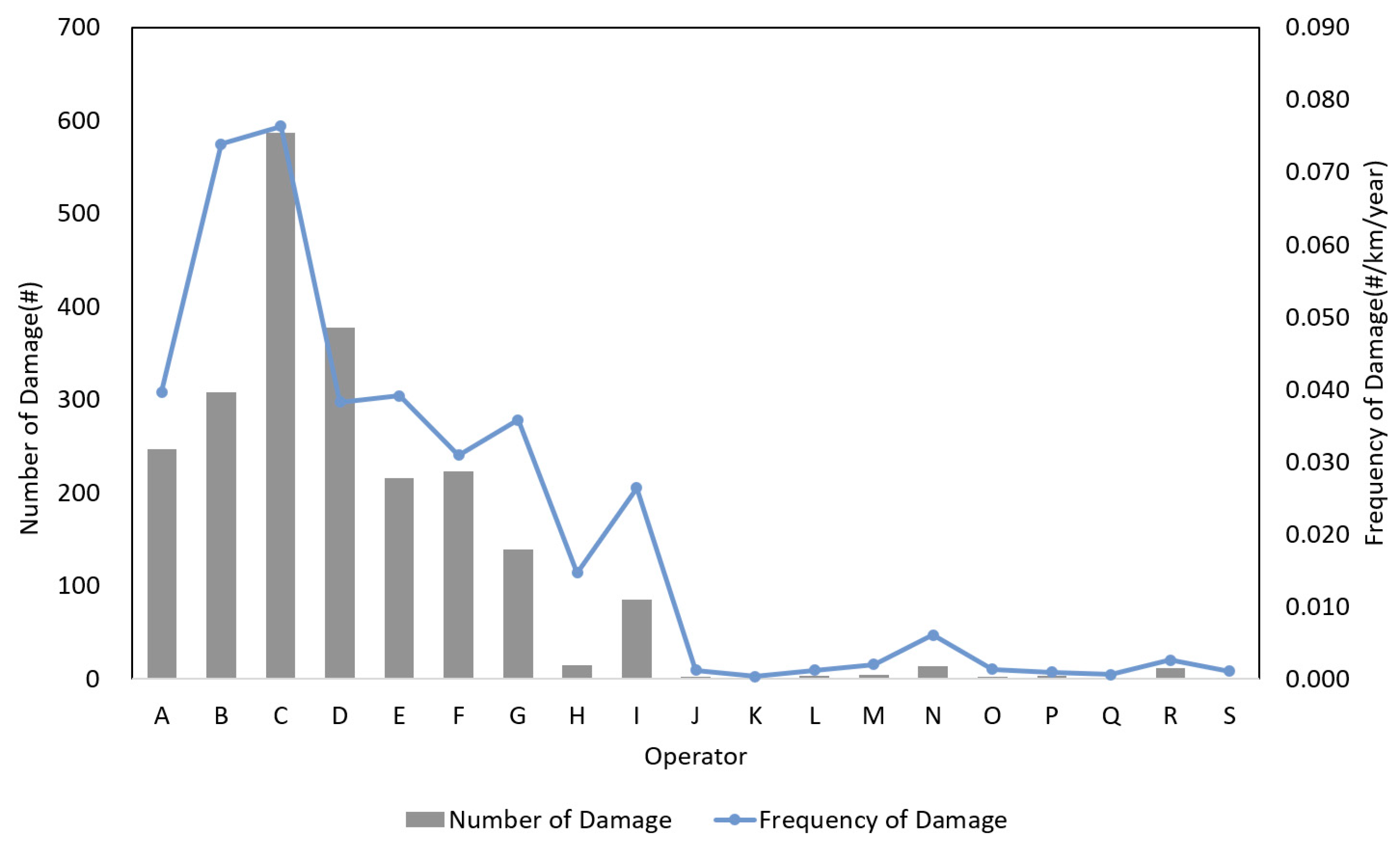
3.2. Operator
3.3. Pipe Function
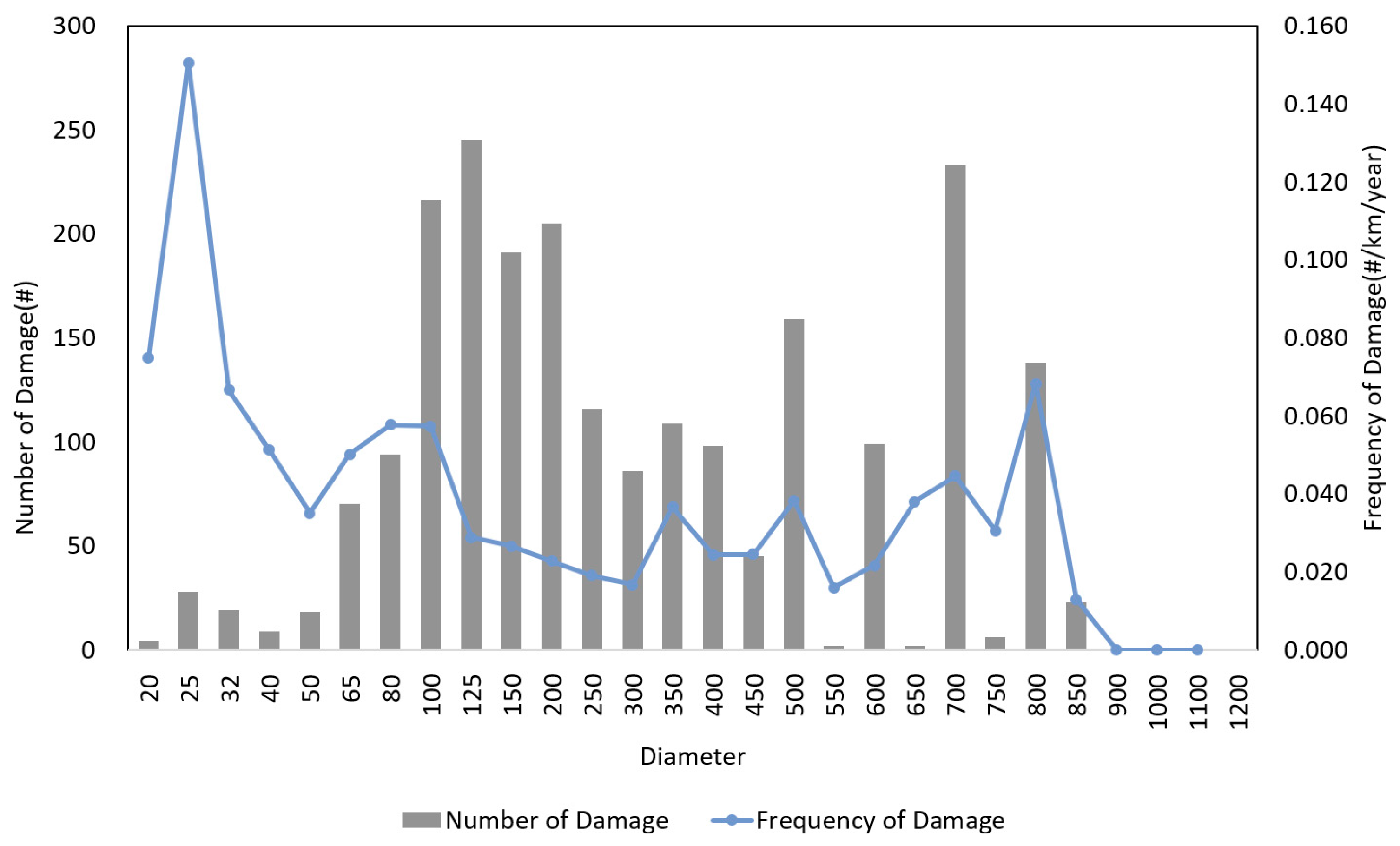
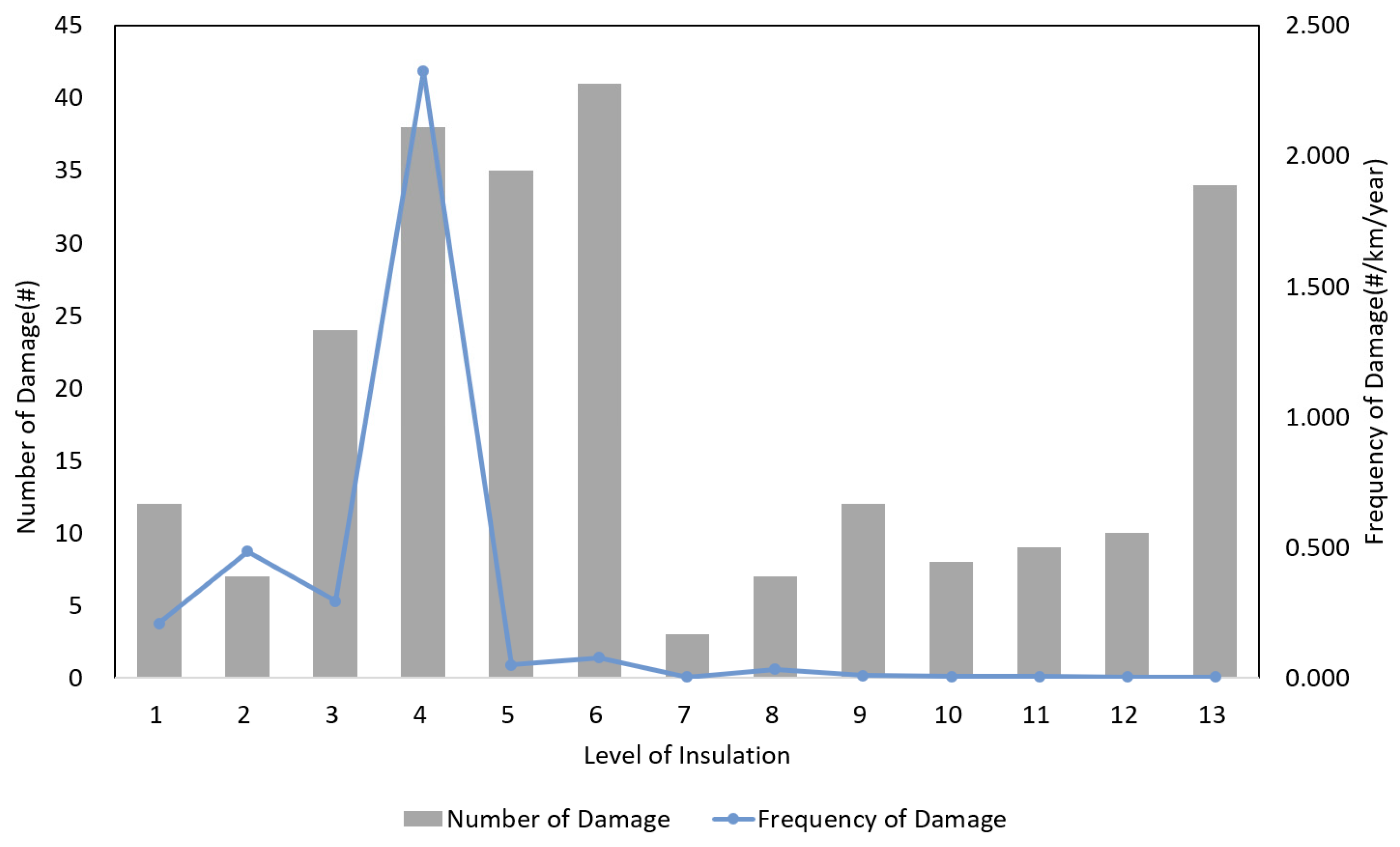
3.4. Pipe Diameter
3.5. Sensor Wire Condition
4. Heat Transport Pipeline Damage Probability Model
4.1. Dataset
4.1.1. Input Data
4.1.2. Output Data
4.2. Data Correlation Analysis
4.3. ML Model
4.3.1. RF
4.3.2. XGBoost (eXtreme Gradient Boosting)
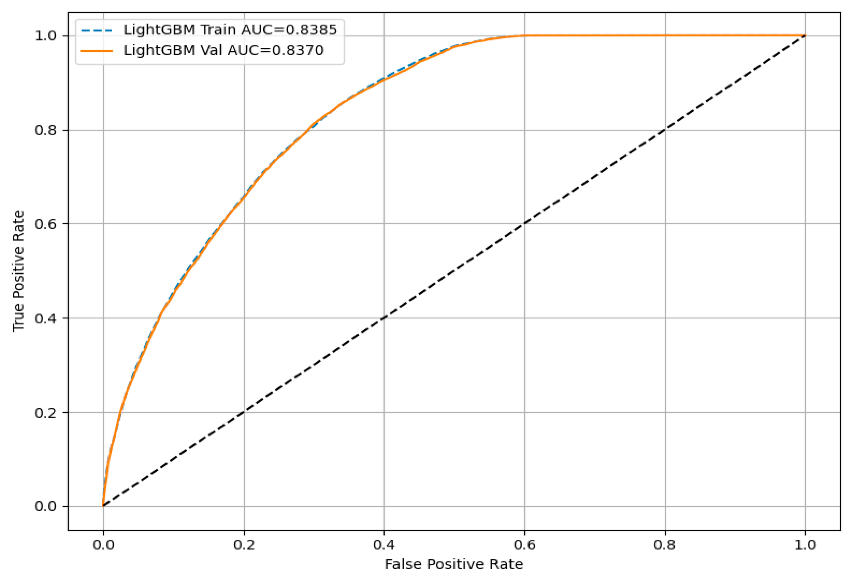
4.3.3. LightGBM (Light Gradient Boosting Machine)
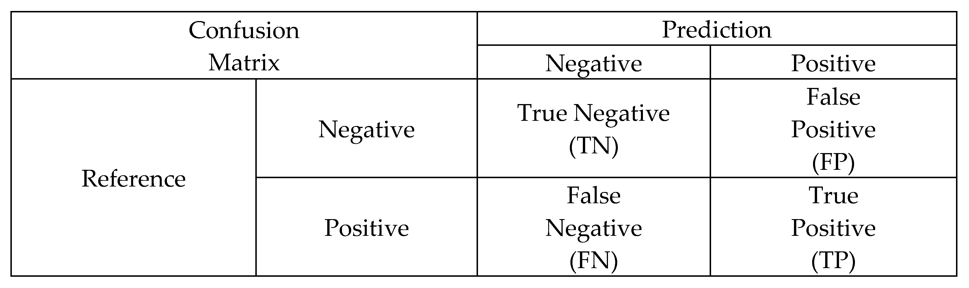
4.4. Model Evaluation Indicators
4.5. Results of Models for Predicting Heat Transport Pipeline Damage Probability
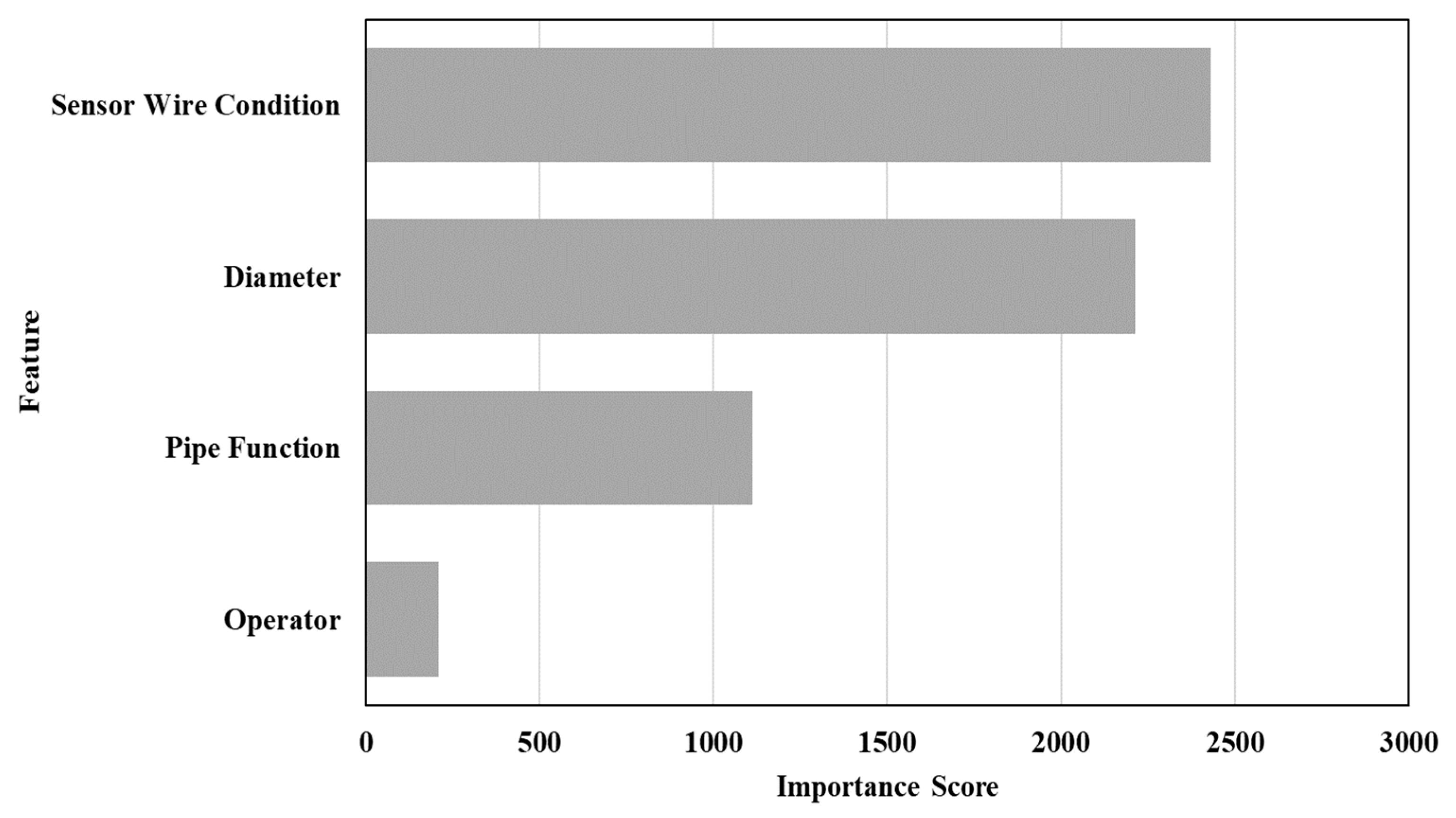
4.6. Importance Analysis
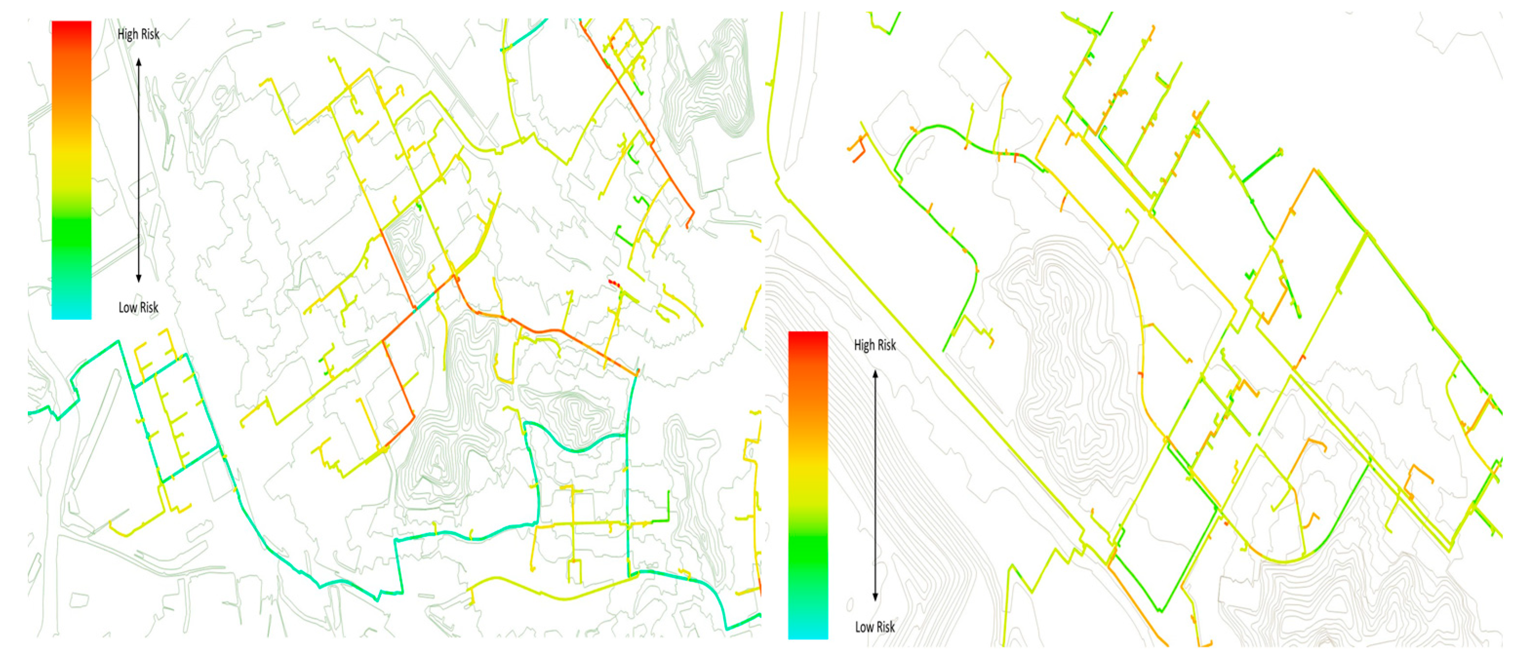
4.7. Visualization of Heat Transport Pipeline Damage Probability
5. Discussion
6. Conclusions
Author Contributions
Funding
Institutional Review Board Statement
Informed Consent Statement
Data Availability Statement
Conflicts of Interest
Abbreviations
| AUC | Area under the curve |
| LGBM | Light Gradient Boosting Machine |
| LightGBM | Light gradient boosting machine |
| ML | Machine learning |
| RF | Random Forest |
| ROC | Receiver Operating Characteristic |
References
- Zhou, S.; O’Neill, Z.; O’Neill, C. A Review of Leakage Detection Methods for District Heating Networks. Appl. Therm. Eng. 2018, 137, 567–574. [Google Scholar] [CrossRef]
- Rafati, A.; Shaker, H.R. Predictive Maintenance of District Heating Networks: A Comprehensive Review of Methods and Challenges. Therm. Sci. Eng. Prog. 2024, 53, 102722. [Google Scholar] [CrossRef]
- van Dreven, J.; Boeva, V.; Abghari, S.; Grahn, H.; Al Koussa, J.; Motoasca, E. Intelligent Approaches to Fault Detection and Diagnosis in District Heating: Current Trends, Challenges, and Opportunities. Electronics 2023, 12, 1448. [Google Scholar] [CrossRef]
- Igwenagu, U.T.I.; Debnath, R.; Ahmed, A.A.; Alam, M.J.B. An Integrated Approach for Earth Infrastructure Monitoring Using UAV and ERI: A Systematic Review. Drones 2025, 9, 225. [Google Scholar] [CrossRef]
- Ravindran, G. Evaluation of New Technologies to Support Asset Management of Metro Systems; UCL Press: London, UK, 2020. [Google Scholar]
- Guan, H.; Xiao, T.; Luo, W.; Gu, J.; He, R.; Xu, P. Automatic Fault Diagnosis Algorithm for Hot Water Pipes Based on Infrared Thermal Images. Build. Environ. 2022, 218, 109111. [Google Scholar] [CrossRef]
- Adegboye, M.A.; Fung, W.-K.; Karnik, A. Recent Advances in Pipeline Monitoring and Oil Leakage Detection Technologies: Principles and Approaches. Sensors 2019, 19, 2548. [Google Scholar] [CrossRef] [PubMed]
- Shen, Y.; Chen, J.; Fu, Q.; Wu, H.; Wang, Y.; Lu, Y. Detection of District Heating Pipe Network Leakage Fault Using UCB Arm Selection Method. Buildings 2021, 11, 275. [Google Scholar] [CrossRef]
- Valinčius, M.; Žutautaitė, I.; Dundulis, G.; Rimkevičius, S.; Janulionis, R.; Bakas, R. Integrated Assessment of Failure Probability of the District Heating Network. Reliab. Eng. Syst. Saf. 2015, 133, 314–322. [Google Scholar] [CrossRef]
- Kong, M.; Kang, J. Methodology for Estimating the Probability of Damage to a Heat Transmission Pipe. J. Korean Geo-Environ. Soc. 2021, 22, 15–21. (In Korean) [Google Scholar]
- Langroudi, P.P.; Weidlich, I. Applicable Predictive Maintenance Diagnosis Methods in Service-Life Prediction of District Heating Pipes. Environ. Clim. Technol. 2020, 24, 294–304. [Google Scholar] [CrossRef]
- Pishvaie, M.R.; Hadipoor, M.; Jafari, S.; Baghery, S. Intelligent Approaches to Fault Detection and Diagnosis in District Heating Systems: A Review. Processes 2023, 11, 2512. [Google Scholar]
- Tol, H.İ.; Madessa, H.B. Enhancing District Heating System Efficiency: A Review of Return Temperature Reduction Strategies. Appl. Sci. 2025, 15, 2982. [Google Scholar] [CrossRef]
- Lee, Y.H.; Kim, S.H.; Kang, U.S.; Kim, W.C.; Kim, J.G. Evaluation of Electrochemical Properties and Life Prediction of Sensor Wire in Leak Detection Systems of Underground Heating Pipelines. J. Electrochem. Soc. 2024, 171, 103508. [Google Scholar] [CrossRef]
- Lidén, P.; Adl-Zarrabi, B.; Hagentoft, C.E. Diagnostic Protocol for Thermal Performance of District Heating Pipes in Operation, 2: Estimation of Present Thermal Conductivity in Aged Pipe Insulation. Energies 2021, 14, 5302. [Google Scholar] [CrossRef]
- Song, S.; Kim, J. Advanced Monitoring Technology for District Heating Pipelines Using Fiberoptic Cable. In Proceedings of the 15th International Symposium on District Heating and Cooling, Seoul, Republic of Korea, 4–7 September 2016; pp. 1–8. [Google Scholar]
- Rahman, A. Statistics-Based Data Preprocessing Methods and Machine Learning Algorithms for Big Data Analysis. Int. J. Artif. Intell. 2019, 17, 44–65. [Google Scholar]
- Bilal, M.; Ali, G.; Iqbal, M.W.; Anwar, M.; Malik, M.S.A.; Kadir, R.A. Auto-prep: Efficient and Automated Data Preprocessing Pipeline. IEEE Access 2022, 10, 107764–107784. [Google Scholar] [CrossRef]
- Khan, L.R.; Tee, K.F. Risk-Cost Optimization of Buried Pipelines Using Subset Simulation. J. Infrastruct. Syst. 2016, 22, 04016001. [Google Scholar] [CrossRef]
- Ebenuwa, A.U.; Tee, K.F. Fuzzy Reliability and Risk-Based Maintenance of Buried Pipelines Using Multiobjective Optimization. J. Infrastruct. Syst. 2020, 26, 04020008. [Google Scholar] [CrossRef]
- Asuero, A.G.; Sayago, A.; González, A.G. The Correlation Coefficient: An Overview. Crit. Rev. Anal. Chem. 2006, 36, 41–59. [Google Scholar] [CrossRef]
- Xu, H.; Deng, Y. Dependent Evidence Combination Based on Shearman Coefficient and Pearson Coefficient. IEEE Access 2018, 6, 11634–11640. [Google Scholar] [CrossRef]
- Tai, J.; Che, C. Automated Machine Learning: A Survey of Tools and Techniques. J. Ind. Eng. Appl. Sci. 2024, 2, 71–76. [Google Scholar] [CrossRef]
- Wählby, U.; Jonsson, E.N.; Karlsson, M.O. Comparison of Stepwise Covariate Model Building Strategies in Population Pharmacokinetic-Pharmacodynamic Analysis. AAPS PharmSciTech. 2002, 2002, 68–79. [Google Scholar] [CrossRef] [PubMed]
- Breiman, L.; Friedman, J.; Stone, C.; Olshen, R. Classification and Regression Trees; Taylor & Francis: Oxfordshire, UK, 1984. [Google Scholar]
- Pal, M. Random Forest Classifier for Remote Sensing Classification. Int. J. Remote Sens. 2005, 26, 217–222. [Google Scholar] [CrossRef]
- Park, E.J.; Park, J.H.; Kim, H.H. Mapping Species-Specific Optimal Plantation Sites Using Random Forest in Gyeongsangnam-do Province, South Korea. J. Agric. Life Sci. 2019, 53, 65–74. (In Korean) [Google Scholar] [CrossRef]
- Hastie, T.; Tibshirani, R.; Friedman, J. The Elements of Statistical Learning: Data Mining, Inference, and Prediction, 2nd ed.; Springer: Berlin/Heidelberg, Germany, 2009; p. 745. [Google Scholar]
- Tian, S.; Zhang, X.; Tian, J.; Sun, Q. Random Forest Classification of Wetland Landcovers from Multy-Sensor Data in the Arid Region of Xinjiang, China. Remote Sens. 2016, 8, 954. [Google Scholar] [CrossRef]
- Lee, S.H.; Yoon, Y.A.; Jung, J.H.; Sim, H.S.; Chang, T.W.; Kim, Y.S. A Machine Learning Model for Predicting Silica Concentrations through Time Series Analysis of Mining Data. J. Korean Soc. Qual. Manag. 2020, 48, 511–520. [Google Scholar]
- Louppe, G. Understanding Random Forests; University of Liege: Leige, Belgium, 2014; p. 211. [Google Scholar]
- Chen, T.; Guestrin, C. XGBoost: A Scalable Tree Boosting System, KDD’16. In Proceedings of the 22nd ACM SIGKDD International Conference on Knowledge Discovery and Data Mining, San Francisco, CA, USA, 13–17 August 2016; pp. 785–794. [Google Scholar]
- Zhang, Y.; Haghani, A. A Gradient Boosting Method to Improve Travel Time Prediction. Emerg. Technol. 2015, 58, 308–324. [Google Scholar] [CrossRef]
- Zhang, D.; Chen, H.D.; Zulfiqar, H.; Yuan, S.S.; Huang, Q.L.; Zhang, Z.Y.; Deng, K.J. iBLP: An XGBoost-Based Predictor for Identifying Bioluminescent Proteins. Comp. Math. Methods Med. 2021, 2021, 6664362. [Google Scholar] [CrossRef] [PubMed]
- Ke, G.; Meng, Q.; Finley, T.; Wang, T.; Chen, W.; Ma, W.; Ye, Q.; Liu, T. LightGBM: A Highly Efficient Gradient Boosting Decision Tree. In Proceedings of the Advances in Neural Information Processing Systems 30 (NIPS 2017), Long Beach, CA, USA, 4–9 December 2017; NeurIPS: La Jolla, CA, USA, 2017; Volume 30. [Google Scholar]
- Ke, G.; Meng, Q.; Finley, T.; Wang, T.; Chen, W.; Ma, W.; Ye, Q.; Liu, T.-Y. LightGBM: A Highly Efficient Gradient BoostingDecision Tree. Adv. Neural Inf. Process. Syst. 2017, 30, 3149–3157. [Google Scholar]
- Lv, J.; Wang, C.; Gao, W.; Zhao, Q. An Economic Forecasting Method Based on the LightGBM-Optimized LSTM and Time-Series Model. Hindawi Comput. Intell. Neurosci. 2021, 2021, 10. [Google Scholar] [CrossRef] [PubMed]
- Gu, Q.; Zhu, L.; Cai, Z. Evaluation Measures of the Classification Performance of Imbalanced Data Sets. In Proceedings of the ISICA 2009—The 4th International Symposium on Computational Intelligence and Intelligent Systems, Communications in Computer and Information Science, Huangshi, China, 23–25 October 2009; Cai, Z., Li, Z., Kang, Z., Liu, Y., Eds.; Springer: Berlin/Heidelberg, Germany, 2009; Volume 51, pp. 461–471. [Google Scholar] [CrossRef]
- Bekkar, M.; Djemaa, H.K.; Alitouche, T.A. Evaluation Measures for Models Assessment over Imbalanced Data Sets. J. Inf. Eng. Appl. 2013, 3, 27–38. [Google Scholar]
- Gietz, H.; Sharma, J.; Tyagi, M. Machine Learning for Automated Sand Transport Monitoring in a Pipeline Using Distributed Acoustic Sensor Data. IEEE Sens. J. 2024, 24, 22444–22457. [Google Scholar] [CrossRef]
- Chen, X.; Karin, T.; Jain, A. Automated Defect Identification in Electroluminescence Images of Solar Modules. Sol. Energy 2022, 242, 20–29. [Google Scholar] [CrossRef]
- Fawcett, T. An Introduction to ROC Analysis. Pattern Recognit. Lett. 2006, 27, 861–874. [Google Scholar] [CrossRef]
- Cawley, G.C.; Talbot, N.L.C. On Over-Fitting in Model Selection and Subsequent Selection Bias in Performance Evaluation. J. Mach. Learn. Res. 2010, 11, 2079–2107. [Google Scholar]
- Vega, A.; Yarahmadi, N.; Jakubowicz, I. Determination of the Long-Term Performance of District Heating Pipes through Accelerated Ageing. Polym. Degrad. Stab. 2018, 153, 15–22. [Google Scholar] [CrossRef]
- Guo, X.; Fu, Q.; Hang, Y.; Lu, H.; Gao, F.; Si, J. Spatial Variability of Soil Moisture in Relation to Land Use Types and Topographic Features on Hillslopes in the Black Soil Area of Northeast China. Sustainability 2020, 12, 3552. [Google Scholar] [CrossRef]
- Kim, S.; Lee, H.; Woo, N.C.; Kim, J. Soil Moisture Monitoring on a Steep Hillside. Hydrol. Processes. 2007, 21, 2910–2922. [Google Scholar] [CrossRef]
- Kim, M.S.; Onda, Y.; Kim, J.K.; Kim, S.W. Effect of Topography and Soil Parameterisation Representing Soil Thicknesses on Shallow Landslide Modelling. Quat. Int. 2015, 384, 91–106. [Google Scholar] [CrossRef]

| Attribute Information | Data Characteristics |
|---|---|
| GIS location information | Shape file |
| Equipment ID | Numeric string |
| Operator | Character string |
| Pipe function | Character string |
| Pipe diameter | Numeric string |
| Installation date | Numeric string |
| Sensor wire condition | Character string |
| Pipe Function | Average Period of Use (Year) | Pipe Length (km) | Number of Damage Cases (#) | Damage Probability (#/km/Year) |
|---|---|---|---|---|
| Supply pipe | 16.00 | 2454.00 | 1557 | 0.043 |
| Return pipe | 16.02 | 2452.26 | 683 | 0.019 |
| Classification | Pipe Length (km) | Number of Damage Cases (#) | Damage Probability (#/km/Year) |
|---|---|---|---|
| Small diameter | 2228.41 | 1099 | 0.034 |
| Medium diameter | 968.40 | 311 | 0.022 |
| Large diameter | 1666.15 | 805 | 0.033 |
| Factor | Pearson Correlation | p-Value |
|---|---|---|
| Operator | −0.302 | 0.000 |
| Pipe function | 0.004 | 0.037 |
| Pipe diameter | −0.204 | 0.000 |
| Sensor wire condition | −0.080 | 0.000 |
| AUC | Evaluation |
|---|---|
| AUC ≧ 0.9 | Excellent |
| 0.8 ≦ AUC < 0.9 | Good |
| 0.7 ≦ AUC < 0.8 | Fair |
| AUC < 0.7 | Poor |
| Dataset | Model | Accuracy | F2-Score | AUC |
|---|---|---|---|---|
| A | XGB | 0.741 | 0.803 | 0.839 |
| LGBM | 0.737 | 0.804 | 0.837 | |
| RF | 0.707 | 0.744 | 0.804 | |
| B | XGB | 0.753 | 0.776 | 0.862 |
| LGBM | 0.741 | 0.781 | 0.861 | |
| RF | 0.714 | 0.726 | 0.832 | |
| C | XGB | 0.768 | 0.730 | 0.901 |
| LGBM | 0.770 | 0.740 | 0.900 | |
| RF | 0.730 | 0.721 | 0.891 |
Disclaimer/Publisher’s Note: The statements, opinions and data contained in all publications are solely those of the individual author(s) and contributor(s) and not of MDPI and/or the editor(s). MDPI and/or the editor(s) disclaim responsibility for any injury to people or property resulting from any ideas, methods, instructions or products referred to in the content. |
© 2025 by the authors. Licensee MDPI, Basel, Switzerland. This article is an open access article distributed under the terms and conditions of the Creative Commons Attribution (CC BY) license (https://creativecommons.org/licenses/by/4.0/).
Share and Cite
Lee, S.; Kang, J.; Kim, J.; Kong, M. AI-Based Damage Risk Prediction Model Development Using Urban Heat Transport Pipeline Attribute Information. Appl. Sci. 2025, 15, 8003. https://doi.org/10.3390/app15148003
Lee S, Kang J, Kim J, Kong M. AI-Based Damage Risk Prediction Model Development Using Urban Heat Transport Pipeline Attribute Information. Applied Sciences. 2025; 15(14):8003. https://doi.org/10.3390/app15148003
Chicago/Turabian StyleLee, Sungyeol, Jaemo Kang, Jinyoung Kim, and Myeongsik Kong. 2025. "AI-Based Damage Risk Prediction Model Development Using Urban Heat Transport Pipeline Attribute Information" Applied Sciences 15, no. 14: 8003. https://doi.org/10.3390/app15148003
APA StyleLee, S., Kang, J., Kim, J., & Kong, M. (2025). AI-Based Damage Risk Prediction Model Development Using Urban Heat Transport Pipeline Attribute Information. Applied Sciences, 15(14), 8003. https://doi.org/10.3390/app15148003