Abstract
The analysis of anomalous diffusion characteristics within single-particle tracking data is a key problem in several applied-science domains, including biosignal processing, bioinformatics, and biotechnology. This task becomes particularly challenging in the presence of short trajectories, localization errors, and non-ergodicity, features that are common in real experimental data. To address these limitations, this work proposes an approach that improves the robustness and accuracy of estimating the anomalous diffusion exponent α, even for very short trajectories of up to 10 points. The approach includes an ensemble-based variance estimation of the exponent α, along with a bias correction based on time–ensemble averaged mean squared displacement, which reduces the systematic bias. These components integrate well into neural network architectures and are suitable for analyzing experimental trajectories in biotechnology and bioprocess engineering applications.
1. Introduction
Optical microscopy has served as a cornerstone tool for studying living cells with minimal invasiveness for centuries, and the emergence of single-molecule techniques over the past two decades has fundamentally transformed cell biology by enabling quantitative characterization of complex cellular dynamics. Among these advances, single-particle tracking (SPT) has established itself as a powerful methodology for the investigation of dynamic processes in life sciences, providing unprecedented access to single-molecule behavior within the natural contexts of living cells and allowing complete statistical characterization of biological systems [1,2,3]. The integration of artificial intelligence approaches in microscopy has further enhanced our ability to analyze the vast datasets generated by SPT experiments, particularly in the characterization of the anomalous diffusion behaviors commonly observed in cellular membranes [4,5]. Anomalous diffusion, characterized by mean squared displacement (MSD) scaling relationships of the form MSD ∝ tα where α ≠ 1, represents a departure from classical Brownian motion and is quantified through ensemble-averaged MSD or time-averaged MSD (TA-MSD) measurements [6,7,8]. However, accurate determination of the anomalous diffusion exponent α presents significant challenges when analyzing the short trajectories typical of SPT experiments, as limited temporal sampling can lead to substantial uncertainties in parameter estimation and potential misclassification of the underlying diffusion mechanism governing molecular transport in living systems.
Research on the statistical properties of the TA-MSD method for estimating anomalous diffusion exponents has primarily focused on analyzing the accuracy, systematic bias, and variance of estimates as functions of observed trajectory length. Studies such as [9,10,11,12] have demonstrated that the variance of anomalous diffusion exponent estimates decreases inversely with increasing trajectory length, yet remains substantial for short time series. Additionally, the properties of time-averaged MSD and its logarithm have emerged as important subjects of analysis, with their characteristics proving critically important for accurate diffusion exponent determination [9,12]. Particular attention has been devoted to systematic bias, which increases for short trajectory lengths and can lead to both overestimation and underestimation of the diffusion exponent [10,11,13]. Beyond theoretical considerations, most studies also provide practical recommendations for applying the TA-MSD method in biophysics, including analysis of the intracellular motion of telomeres, proteins, and other macromolecules [13,14,15].
The Anomalous Diffusion (AnDi) Challenge was organized in 2020 to objectively compare methods for the characterization of anomalous diffusion from particle trajectories [16,17]. An open-source framework was developed to simulate trajectories for training and testing datasets modeled by five distinct diffusion processes [18]. The challenge revealed that for such diverse and complex datasets, machine learning-based methods for estimating anomalous diffusion exponents significantly outperform classical statistical approaches [19]. One of the best, easily applicable neural network approaches identified in the competition was RANDI, which is based on a two-layer long short-term memory structure [20].
The second AnDi Challenge (AnDi-2024) [21] aimed to evaluate methods for detecting and quantifying changes in single-particle motion. A key complication of this challenge was the strong heterogeneity of particle trajectories. In addition, the competition emphasized ensemble-based analyses. Here, “ensemble” refers to a collection of multiple particle trajectories. By analyzing multiple trajectories collectively, researchers were able to significantly improve estimation accuracy.
Unlike the first AnDi Challenge, which involved noisy trajectories generated by five different underlying diffusion models, the second challenge focused exclusively on noise-free trajectories simulated using fractional Brownian motion (fBm). In this more controlled yet demanding setting, we observed that classical statistical methods such as the time-averaged mean squared displacement [22] and Hurst exponent estimators such as the Whittle method [23] performed in a manner comparable to more complex machine learning approaches. Furthermore, classical methods offer a practical advantage since they can be applied directly without the need for training.
The objective of this study is to develop ensemble-based correction methods for improving anomalous diffusion exponent estimation from short single-particle trajectories. Rather than developing new estimation algorithms like [17,20,24], our approach leverages ensemble statistics to correct individual trajectory estimates, following the paradigm of ensemble-based reliability enhancement, similar to [25]. By using collective information across multiple particles, we compensate for the noise and bias inherent in single-trajectory analysis, extending the reliability of existing methods to challenging short-trajectory regimes.
Our contributions are as follows:
- Variance-Based Ensemble Estimation: For any α estimation method, we propose empirically characterizing the method-specific noise component σ2 (α, trajectory length) to enable shrinkage correction, optimally balancing individual trajectory information with ensemble statistics to improve estimation accuracy and robustness.
- Bias Correction in Short Trajectories: In normal and superdiffusive regimes, finite-length effects can introduce systematic biases into exponent estimates, especially when trajectories are extremely short. To address this, we propose using the time–ensemble averaged mean squared displacement (TEA-MSD) as a more reliable and length-invariant method for characterizing diffusion behavior in fractional Brownian motion. This approach enables accurate correction of the ensemble mean.
- All code and experimental results supporting the findings of this study are publicly available at: github.com/SophiaLavr/Correction-AnDi-Exponent (accessed on 17 July 2025).
2. Materials and Methods
2.1. The TA-MSD Method and Its Statistical Characteristics
The mean squared displacement over a time interval Δ is defined as the expected value of the squared particle displacement. In the two-dimensional case in the x- and y-coordinate planes, the MSD is defined as
where t is the time, and Δ is the time interval over which the displacement is measured.
For anomalous diffusion, the relationship between MSD and time Δ is expressed as
where α is the anomalous diffusion exponent. This relationship characterizes anomalous diffusion, where α = 1 corresponds to normal diffusion, α < 1 to subdiffusion, and α > 1 to superdiffusion.
The estimation of anomalous diffusion exponents from single-particle trajectories is commonly performed using time-averaged mean square displacement (TA-MSD) analysis. For a two-dimensional trajectory (X, Y) with time interval between observations δt, the TA-MSD is given by
where T is the length of the particle trajectory, defined as the total number of discrete data points (i.e., time steps) over which the particle was tracked, and τ is an integer multiple of the basic time step δt and represents the discrete time lag. For the method to be applicable, the condition T ≫ τ must hold. Estimation of the anomalous diffusion exponent α is achieved according to Formula (2), by logarithmic transformation of TAMSD(τ) versus τ. This yields a linear relation in logarithmic coordinates, and the slope of the regression corresponds to the estimate of the anomalous diffusion exponent α.
Previous studies [9,11,12,13] have investigated the dependence of the estimation of on the trajectory length T and shown that when estimating exponent α by the TA-MSD method, the variance of the estimation is inversely proportional to the value of T:
To estimate the variance of for the TA-MSD method in Formula (3), the estimate is obtained through linear regression in a logarithmic scale:
where log refers to a logarithm with an arbitrary base. In the two-dimensional case, since the displacements along the x- and y-coordinates are assumed to be independent, the variance of the increments is given by the sum of the variances along each direction. To estimate the variance of the exponent α, we use an approximate formula for the variance of the logarithm of a random variable based on the error propagation formula [26]:
where Z = TAMSD(τ). Based on Formula (6) and considering that for fractional Brownian motion, ] = and , it can be shown that the approximate relation is satisfied when T ≫ τ:
Var[log(TAMSD(τ))] ≈ 1/T
In this case, the determination takes into account that the estimation of α is performed using a linear regression of the TAMSD as a function of τ in log–log scale:
where K is the number of lags τ, and the overbar notation represents the arithmetic average.
2.2. Ensemble-Based Correction of TA-MSD Estimates
Consider an ensemble of trajectories of fixed length T, generated using fractional Brownian motion with a given diffusion exponent α. When estimating the diffusion exponent α using the TA-MSD method, we obtain an estimate of the diffusion exponent, the variance of which is inversely proportional to the trajectory length according to Formula (7). Let us denote the variance of the estimate obtained by the TA-MSD method as . This quantity corresponds to the variance in Formula (8).
In the context of the AnDi-2024 Challenge, it is assumed that when generating an ensemble of trajectories, the diffusion exponent α is a random variable with normal distribution α ~ N(μα, σ2α). In this case, the total variance of the diffusion exponent estimate will depend on both the estimation method error and the spread of the parameter α itself. Thus, the observed variance in the estimates of the exponent α for ensemble trajectories can be expressed as
When , we can assume that = 0, and all trajectories in the ensemble have the same value of exponent α = μα. We can also estimate the variance of the normal distribution for exponent α if we estimate the total variance and the estimation variance :
In such cases, normalizing the individual trajectory estimates relative to the ensemble-averaged estimate can improve accuracy.
Note that according to Formula (8), the value of depends on the number of selected lags for τ. For example, for the set τ = {1, 2, 3, 4}, considering that , the variance can be represented as
The experimental results shown in Figure A1 (Appendix A) reveal good agreement between the experimentally determined dependency coefficient and the value calculated using Equation (11).
The correction method proceeds as follows. For each i-th trajectory (i = 1, M) from the ensemble of realizations, we obtain an estimate of the exponent and calculate the mean value and variance estimate :
Consider an initial estimate of a parameter, denoted as , which is modeled as a random variable following a normal distribution: ∼ N(,). Our objective is to transform into a new random variable, , which represents a refined or “corrected” estimate. This corrected estimate is also assumed to follow a normal distribution, ∼ N(,), where its variance is derived from Equation (10) as [13].
To implement this transformation while preserving the normal distribution, we employ a linear transformation, a well-established technique for normally distributed random variables [27,28]. For a general random variable P1∼N(μ1, σ12) and a desired transformed variable P2∼N(μ2, σ22), the linear transformation is defined as
This formula ensures that the transformed variable P2 has the desired mean μ2 and variance σ22. The term σ2/σ1 acts as a scaling factor, adjusting the spread of the distribution, while the addition of μ2 and subtraction of μ1 shift the mean. Applying this transformation to our case,
where is the original estimate of the anomalous diffusion exponent for the i-th trajectory, and is the corrected estimate of α for the i-th trajectory.
2.3. TEA-MSD for Correction of TA-MSD Estimates
Studies [10,13,14,15] have shown that for short trajectories, estimates of the anomalous exponent α obtained by the TA-MSD method for fBm trajectories exhibit systematic bias. These works demonstrate that for small trajectory lengths, the estimate can be systematically overestimated or underestimated depending on the true α and method parameters. The bias arises from the limited number of points available for averaging, correlations in fBm, and the sensitivity of logarithmic regression to statistical fluctuations.
For an ensemble of trajectories with short lengths, averaging the per-trajectory estimates over the ensemble and comparing this result with the true value α used in generation reveals systematic underestimation, especially for large values of α.
To address this problem, we calculate the diffusion exponent estimate for the entire ensemble by using the TEA-MSD method [29], which includes averaging over both ensemble and time, providing a single estimate for the entire ensemble. The time–ensemble averaged mean square displacement TEAMSD(τ) is defined as
where M is the number of trajectories in the ensemble. Estimation of the anomalous diffusion exponent is achieved by creating a log–log plot of TEAMSD(τ) versus time lag τ. The slope of this line estimates the anomalous diffusion exponent, .
Studies [13,15] have shown that TEA-MSD, with a sufficient number of trajectories, provides significantly less bias than TA-MSD, because ensemble averaging reduces the influence of fluctuations. Thus, the estimate obtained using (16) corresponds quite closely to the true value of α, even for short trajectories.
In this case, we can use the obtained ensemble estimate to refine the per-trajectory estimates , obtaining the following modified formula:
This approach maintains simplicity, eliminates the need for additional model training, and significantly improves the reliability of the TA-MSD method used for analyzing ensembles of short particle trajectories in complex systems.
2.4. Generalization of Ensemble-Based Correction
The correction of exponent α estimates can also be performed for cases in which the estimates are obtained not through TA-MSD, but by any other method, including both classical statistical methods and modern machine learning methods, such as neural networks. It is important to have empirical information about the dependence of the variance of α estimates on the trajectory length T, as well as the ensemble mean value; this dependence can be obtained by various methods. Such information allows the correction of predictions made using any α estimation methods, based on knowledge of the error structure arising from limited trajectory length.
We propose the following numerical approach. For a set of fixed values of α and various values of trajectory length T from the range of interest, an ensemble of trajectories is generated (e.g., several thousand for each pair {α, T}). After estimating α for each trajectory from the ensemble and obtaining estimates , the sample variance of estimates corresponding to the given pair of values {α, T} is calculated. Since all generated trajectories in the ensemble have the same specified α value, , and therefore . This allows the obtaining of the dependence of the empirical values on T.
Then, for each fixed value of α, we perform linear regression to study how the estimate variance depends on 1/T. This helps reveal how the variance changes as the trajectory length increases. Once we have a set of linear relationships for different values of α, we can build an approximating function that takes T and a given estimate as inputs. Using parametric interpolation over α, this function allows us to calculate the expected value for the variance estimate .
Correction of estimates obtained by a specific method, for which we now have a function that provides from T and , is performed using the following modification of Formula (17):
Thus, we correct the estimates of anomalous exponents for each trajectory obtained by a specific method.
Appendix B provides examples of the determinations of anomalous diffusion parameters for the TA-MSD, Whittle, and CINNAMON methods (based on machine learning and independent of trajectory length) [30], illustrating that the dependence of alpha variance on 1/T can be approximated by linear regression.
3. Results
3.1. TEA-MSD Estimation Test
In this subsection, we evaluate the effectiveness of the TEA-MSD method (Section 2.3) compared to the averaging estimates obtained from other methods. For this comparison, besides the TA-MSD method (Section 2.1), we selected the Whittle method [23] (implemented to compute a Hurst exponent estimator using maximum likelihood on the periodogram, which is effective for fBM). From among the neural network-based approaches, we selected the RANDI deep learning model [20], recognized as one of the top-performing methods in the challenge. To ensure compatibility with the published trained models of RANDI, we generated a synthetic two-dimensional AnDi-2024 dataset with trajectory lengths of 25 points.
Ensemble trajectories were simulated from fractional Brownian motion processes, with α following a normal distribution N(μ, σ2) bounded between 0 and 2. The truncation was performed using the scipy.stats.truncnorm.rvs function in SciPy, which generates random variates only from the portion of the normal distribution within the specified bounds, using an efficient sampling algorithm that avoids simple rejection sampling. Conventional methods, including the machine learning-based approaches used in AnDi, estimate each trajectory individually. The parameter μ can be estimated by taking the mean value of the individual estimates. By applying the TEA-MSD approach, we can directly obtain a single estimate for the entire ensemble. We experimentally verify how the effectiveness of μ estimation methods differs for various values of μ and σ. The mean absolute error (MAE) metric, as adopted in the AnDi competition, is used to evaluate performance.
For all our experiments, we adopted K = 4 (the number of lags τ). This choice was primarily dictated by the conditions of the AnDi-2024 Challenge, on the benchmark dataset of which we evaluated our method; in this dataset, trajectories frequently consist of only several dozen points, and can be as short as four points.
The results (Figure 1) show that for small and moderate values of σ, TEA-MSD (red line) outperforms the other methods. In cases where σ is high, transforming the truncated normal distribution over the interval [0,2] into an almost uniform distribution, the effectiveness of all methods significantly decreases, making it difficult to select the best among them. Thus, the application of TEA-MSD instead of averaging individual trajectory α estimates demonstrates its effectiveness in this experiment. The experiments were carried out using two distinct configurations. In the first, the diffusion coefficient D was kept constant across all trajectories in the ensemble, while in the second, D was independently assigned to each trajectory as a random value drawn from a normal distribution with high variance. Despite these differences, the results showed no significant variation between the two setups. The TEA-MSD method demonstrated a similar level of accuracy in estimating μ in both cases, suggesting that it is not sensitive to variations in D, even when those variations are substantial.
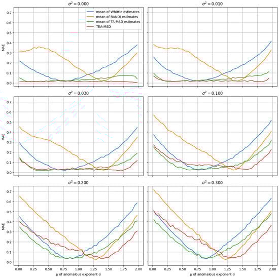
Figure 1.
Dependence of MAE(μ) on μ for different values of σ, comparing methods for estimating the anomalous diffusion exponent (through averaging α values for ensemble trajectories and the TEA-MSD method).
These two configurations were also applied in the experiments detailed in Section 3.2 and Section 3.3, the consistency of the results of which further supported the conclusion that the performance of our correction framework remains stable regardless of the specific distribution or variability of the diffusion coefficient D.
All code and experimental results are publicly available in the following repository: github.com/SophiaLavr/Ensemble-Based-Correction-for-Anomalous-Diffusion-Exponent-Estimation.
3.2. TA-MSD Correction Method Test
In this subsection, we perform an experimental comparison of the proposed corrected time-averaged MSD method described in Formula (17) and the classical TA-MSD method, the Whittle method, and the α exponent estimation obtained using the RANDI neural network approach.
Ensemble trajectories were generated with α following a truncated normal distribution N(μ, σ2), bounded between 0 and 2. Applying the TEA-MSD approach for μ estimation and trajectory correction based on the dependence of the TA-MSD method estimation variance on T, we experimentally evaluate the effectiveness of the correction compared to conventional trajectory α estimation methods for various μ and σ values. The trajectory length of T = 25 was specifically chosen to ensure compatibility with the RANDI neural network model, which is trained on trajectories of this particular length.
The results (Figure 2) show that for small and moderate values of σ, corrected estimates outperform other methods in terms of the MAE metric. However, as σ increases, the truncated normal distribution over [0,2] becomes progressively flattened, leading to a less distinct peak and a shape that deviates increasingly from a typical Gaussian profile. In such cases, the effectiveness of the correction method diminishes significantly, and the conventional TA-MSD method becomes more reliable. This is because attempting to correct trajectories that are not normally distributed only worsens the results, demonstrating the limitations in the correction method’s application
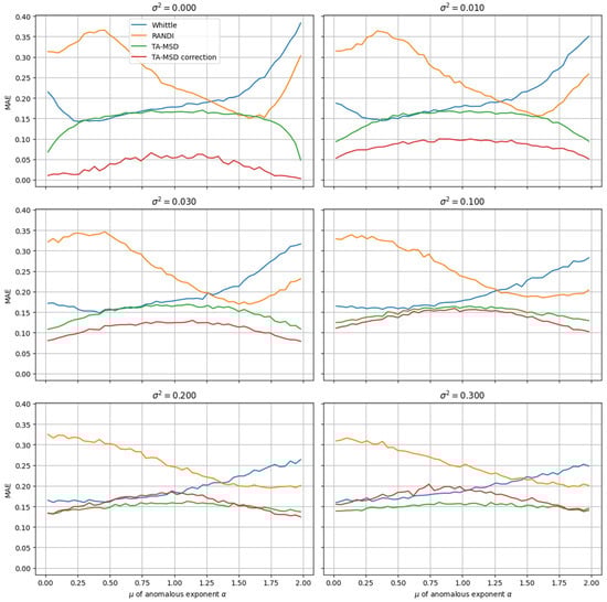
Figure 2.
Dependence of MAE of ensemble trajectory α estimates on μ and σ for estimation methods and the correction method.
3.3. Generalization of the Correction Approach to Other α Estimation Methods
Here we present the experimental results demonstrating the generalization of the correction approach outlined in Section 2.4. The correction is performed using Formulas (17) and (18).
Appendix B shows how linear dependencies of Var(α) on 1/T were established for several μ values for three methods: TA-MSD (baseline), the Whittle method (based on periodograms, effective for fBm), and Cinnamon (based on machine learning but, unlike RANDI, independent of trajectory length). The investigated methods differ in their underlying approaches. The trajectory length range is selected according to the working range of the task. For subsequent use on the AnDi-2024 dataset (Section 3.4), in which the typical trajectory lengths are composed of several dozen points (with a minimum of 4 points and a maximum of 200), we selected a trajectory length range of T = 16 to T = 50 points for our detailed analysis. Given our choice of K = 4 (number of lags τ), we specifically limited our experimental analysis to trajectory lengths starting from T = 16. This ensures that K ≤ T/4, a condition under which the estimation remains stable and consistent. We observed that computational instability and increased estimation variance occur when K exceeds approximately T/4. This behavior is attributed to the decreasing number of independent segments available for reliable MSD averaging at larger lag times τ, which leads to TA-MSD estimates that are less reliable. It is important to note that the established dependency between T and Var(α) within this range is expected to hold true for adjacent ranges as well, extending its applicability to both very short trajectories (e.g., from four points) and longer ones (up to several hundreds of points).
For each method (Figure 3), we created a function for estimating Var(α) from μ and T using parametric interpolation. As a result, it is possible to correct the α values of trajectories based on the method-specific variance estimates provided by the function and μ estimates obtained using TEA-MSD.
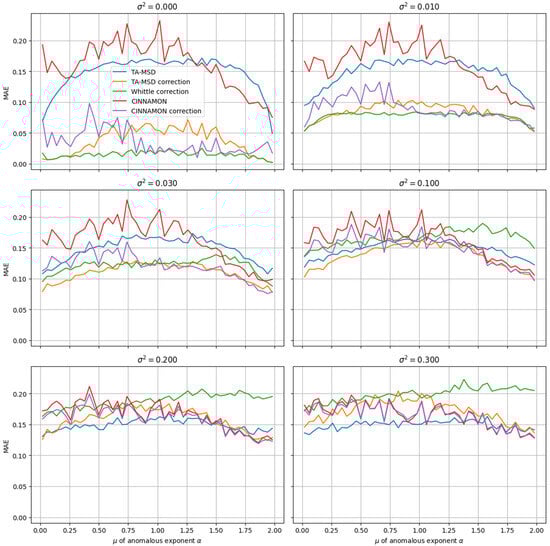
Figure 3.
Dependence of MAE of ensemble trajectory α estimates on μ and σ obtained by correction of estimates from different methods. Results for uncorrected TA-MSD and CINNAMON are also shown. Results for the uncorrected Whittle curve have been omitted for clarity and readability.
The consistent linear relationships across all three methods validate the generalizability of the proposed ensemble-based correction framework, demonstrating its applicability to both classical statistical methods and modern machine learning approaches for anomalous diffusion exponent estimation
Figure 3 demonstrates the correction results across different μ and σ2 values for trajectories with a length of 25, simulated from fractional Brownian motion processes with α following a truncated normal distribution N(μ, σ2) bounded between 0 and 2. The performance comparison includes five methods: TA-MSD (blue line), TA-MSD with correction (orange line), the Whittle method with correction (green line), uncorrected CINNAMON (red line), and CINNAMON with correction (purple line). The inclusion of the uncorrected methods allows for direct assessment of the correction effectiveness.
3.4. Performance Evaluation on the AnDi-2 Benchmark Dataset
To evaluate the practical utility of our method, we conducted two experiments using the second AnDi benchmark dataset [31]. First, we assessed the benefit of ensemble-based correction in our team’s solution submitted to the second AnDi Challenge. Performance was evaluated using the MAE metric, following the standard protocol of the AnDi competition. The results presented in Figure 4 demonstrate that the correction method produces positive outcomes across all three experimental configurations.
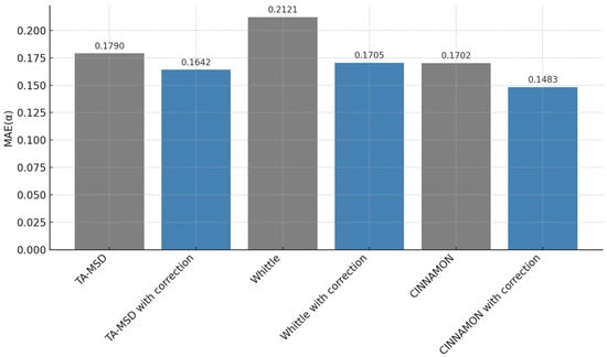
Figure 4.
Performance comparison on the AnDi-2 benchmark dataset showing results for TA-MSD with/without correction, Whittle with/without correction, and Cinnamon with/without correction. The experiments conducted demonstrate the effectiveness of the proposed correction approach, across different estimation methods, on benchmark data.
4. Discussion
Ensemble-based correction methods have clear limitations. If the variance of the diffusion exponent across an ensemble rises above 0.2–0.3, the underlying distribution over [0,2] becomes progressively flattened, leading to a less distinct peak and a shape that deviates increasingly from a typical Gaussian profile. When this happens, the estimation of the true mean becomes unreliable, and using ensemble-based correction can actually make results worse instead of better. Despite this, the method is still practical, especially in ensemble analysis, in which researchers look at multiple trajectories together and can apply these correction techniques.
To avoid performance issues, researchers should only apply the correction when the diffusion exponent’s variance is below the 0.2–0.3 threshold. This targeted approach improves the method’s overall effectiveness by making sure that it is not used in situations where it would be harmful.
We observed that the correction method detailed in Section 2.1, Section 2.2 and Section 2.3 does not perform optimally when K (the number of lags) exceeds approximately T/4, which may limit the applicability of this method in certain scenarios. However, it is important to note that in such cases, the generalized method described in Section 2.4 remains a suitable approach.
The effectiveness of the proposed method, particularly in accurately estimating the ensemble variance (σ2total) and applying the subsequent rescaling correction, depends inherently on the number of trajectories in the ensemble (M). While the TEA-MSD component demonstrates robust performance in estimating the mean diffusion exponent even for relatively small values of M, the reliability of the variance-based correction deteriorates when M falls below a certain threshold. Although we have not explicitly determined this critical minimum value of M within the scope of this study, our results were obtained using ensemble sizes consistent with those found in benchmark datasets such as AnDi-2024, in which M is typically sufficient to ensure stable variance estimation. In experimental settings where only a limited number of trajectories is available, the advantages of our correction approach may be reduced, and its applicability could become constrained.
It is also worth noting that our method demonstrates robustness with respect to variations in the diffusion coefficient D across trajectories within the ensemble. As assumed in the AnDi-2024 challenge framework, the diffusion coefficient D may follow a normal distribution across the ensemble, yet this does not hinder the accurate estimation of the anomalous diffusion exponent α. Our experimental results confirm that the performance of the correction framework remains consistent regardless of whether D is fixed or varies significantly across trajectories.
However, we emphasize that this property is not a novel finding of our study. It has been previously discussed in the literature, specifically in [13], where it was shown that the distribution of the diffusion coefficient does not affect the accurate extraction of the anomalous exponent. We refer interested readers to that work for a more detailed theoretical analysis of this invariance.
Currently, our method has been rigorously validated only on synthetic fBM data. We acknowledge that the direct application of our current method to real SPT data is hindered by the absence of ground truth anomalous diffusion parameters in real-world datasets. This is a common challenge for solutions developed within the AnDi-2024 Challenge, as they are developed and tested on simulated data.
Another significant challenge with respect to real data arises from highly heterogeneous systems (e.g., motion within living cells, tissues, or organisms, where motion types can vary both between and within tracks). Heterogeneity and its detection are, in fact, the central problems that the AnDi-2024 Challenge was organized to address. Specifically, for heterogeneous systems, a prerequisite step would involve segmenting the complex trajectories into homogeneous segments. Only then could a set of α estimates derived from these homogeneous segments be refined by our proposed correction method. Our method is designed to enhance the accuracy of α estimations for ensembles of trajectories that are assumed to be drawn from a single underlying diffusion process, making it an appropriate refinement step after initial segmentation or for inherently homogeneous systems.
Beyond single-particle tracking, this correction method could be useful for estimating the Hurst exponent in time series with gaps or missing data. Since these series cannot be treated as one continuous record, their fragmented parts can be viewed as an ensemble. Our method could then correct the Hurst exponent estimates for each of these segments, extending the use of the method beyond SPT to other areas.
5. Conclusions
This study introduces an ensemble-based correction method to improve the accuracy of anomalous diffusion exponent (α) estimation from short and noisy single-particle tracking data. Our approach combines the robust mean estimation from time–ensemble averaged mean squared displacement with a novel correction that accounts for method-specific variance depending on trajectory length.
Evaluated on synthetic data and the AnDi-2 benchmark, the method significantly reduces bias and mean absolute error for α estimates, particularly for short trajectories, improving the performance of traditional and machine learning based methods.
Author Contributions
Conceptualization, R.L., L.K. and S.L.; methodology, R.L., L.K. and S.Y.; software, R.L., S.L. and N.R.; validation, L.K., S.Y. and N.R.; formal analysis, L.K. and S.Y.; investigation, R.L.; resources, S.L. and N.R.; data curation, R.L., S.L. and N.R.; writing—original draft preparation, R.L., S.L. and N.R.; writing—review and editing, L.K. and S.Y.; visualization, R.L. and S.L.; supervision, L.K. and S.Y.; project administration, S.Y.; funding acquisition, L.K. and S.Y. All authors have read and agreed to the published version of the manuscript.
Funding
The study is funded by the IMPRESS-U programme within the framework of the project “Modeling and forecasting the spread of infection in war and post-war period using epidemiological, behavioral and genomic surveillance data” (2023/05/Y/ST6/00263).
Institutional Review Board Statement
Not applicable.
Informed Consent Statement
Not applicable.
Data Availability Statement
The data used in this study are openly available in AnDi 2 benchmark dataset. Zenodo 2024 at https://doi.org/10.5281/zenodo.14281479 (accessed on 17 July 2025).
Conflicts of Interest
The authors declare no conflicts of interest.
Abbreviations
The following abbreviations are used in this manuscript:
| AnDi | Anomalous Diffusion |
| fBm | Fractional Brownian Motion |
| MAE | Mean Absolute Error |
| MSD | Mean Square Displacement |
| SPT | Single-Particle Tracking |
| TA-MSD | Time-Averaged Mean Squared Displacement |
| TEA-MSD | Time–Ensemble Averaged Mean Square Displacement |
Appendix A
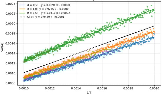
Figure A1.
Dependence of α estimation variance by TA-MSD method on 1/T. For α = 1, the slope of the linear regression line is approximately 0.9275, indicating an approximate dependence Var(α) = 0.9275/T.
We generated 5000 trajectories for each trajectory length value from 1000 to 5000 points for three α values, estimated using the TA-MSD method, and for each length and α, estimated the variance of α estimates. We calculated the parameters of linear regression for the dependence of Var(α) on 1/T. The experimental results (Figure A1) show that the calculated dependence value of 0.9216/T (obtained in Section 2.2) is achieved with sufficiently high accuracy only for Hurst exponent values H close to 0.5. For other values, there are deviations from the calculated values.
The experiment demonstrates that for the specific TA-MSD method, the variance of α estimation depends not only on the series length but also on α itself.
Appendix B
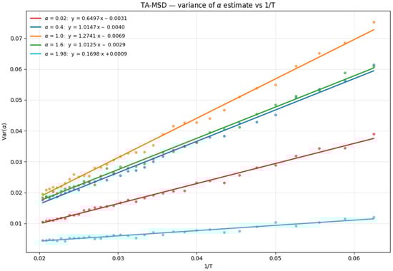
Figure A2.
Var(α) vs. 1/T for TA-MSD method for 5 α values. T range from 16 to 50.
Figure A2 shows the linear relationship between estimation variance and inverse trajectory length for the TA-MSD method across different true α values. The consistent linear patterns validate the theoretical foundation of the correction approach.
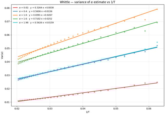
Figure A3.
Var(α) vs. 1/T for Whittle method for 5 α values. T range from 16 to 50.
Similar linear relationships are observed for the Whittle estimator, though with different slopes and intercepts compared to TA-MSD, reflecting the method’s different statistical properties.
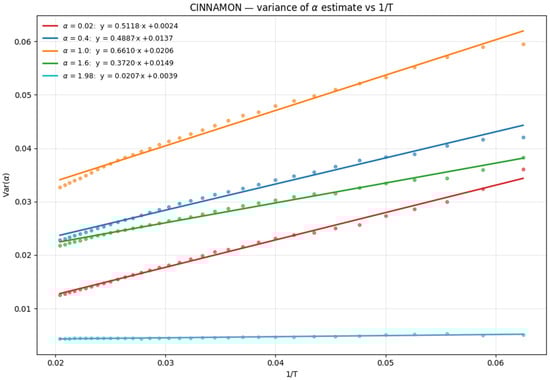
Figure A4.
Var(α) vs. 1/T for CINNAMON method for 5 α values. T range from 16 to 50.
The machine learning-based CINNAMON method also exhibits an almost linear dependence, confirming that the correction framework is applicable across diverse estimation approaches.
References
- Scott, S.; Weiss, M.; Selhuber-Unkel, C.; Barooji, Y.F.; Sabri, A.; Erler, J.T.; Metzler, R.; Oddershede, L.B. Extracting, Quantifying, and Comparing Dynamical and Biomechanical Properties of Living Matter through Single Particle Tracking. Phys. Chem. Chem. Phys. 2022, 25, 1513–1537. [Google Scholar] [CrossRef] [PubMed]
- Manzo, C.; Garcia-Parajo, M.F. A Review of Progress in Single Particle Tracking: From Methods to Biophysical Insights. Rep. Prog. Phys. 2015, 78, 124601. [Google Scholar] [CrossRef] [PubMed]
- Shen, H.; Tauzin, L.J.; Baiyasi, R.; Wang, W.; Moringo, N.; Shuang, B.; Landes, C.F. Single Particle Tracking: From Theory to Biophysical Applications. Chem. Rev. 2017, 117, 7331–7376. [Google Scholar] [CrossRef] [PubMed]
- Krapf, D. Mechanisms Underlying Anomalous Diffusion in the Plasma Membrane; Academic Press: Cambridge, MA, USA, 2015; Volume 75, pp. 167–207. [Google Scholar] [CrossRef]
- Nguyen, T.L.; Chen, Y.; Chen, L.H.; Yeh, H. Recent Advances in Single-Molecule Tracking and Imaging Techniques. Annu. Rev. Anal. Chem. 2023, 16, 253–284. [Google Scholar] [CrossRef]
- Spagnolo, C.S.; Luin, S. Trajectory Analysis in Single-Particle Tracking: From Mean Squared Displacement to Machine Learning Approaches. Int. J. Mol. Sci. 2024, 25, 8660. [Google Scholar] [CrossRef]
- Metzler, R.; Jeon, J.-H.; Cherstvy, A.G.; Barkai, E. Anomalous Diffusion Models and Their Properties: Non-Stationarity, Non-Ergodicity, and Ageing at the Centenary of Single Particle Tracking. Phys. Chem. Chem. Phys. 2014, 16, 24128–24164. [Google Scholar] [CrossRef]
- Weiss, M. Resampling single-particle tracking data eliminates localization errors and reveals proper diffusion anomalies. Phys. Rev. E 2019, 100, 042125. [Google Scholar] [CrossRef]
- Sikora, G.; Teuerle, M.; Wyłomańska, A.; Grebenkov, D. Statistical properties of the anomalous scaling exponent estimator based on time-averaged mean-square displacement. Phys. Rev. E 2017, 96, 022132. [Google Scholar] [CrossRef]
- Burnecki, K.; Kepten, E.; Garini, Y.; Weron, A.; Sikora, G.; Barkai, E. Estimating the anomalous diffusion exponent for single particle tracking data with measurement errors—An alternative approach. Sci. Rep. 2015, 5, 11306. [Google Scholar] [CrossRef]
- Kepten, E.; Weron, A.; Sikora, G.; Burnecki, K.; Garini, Y. Guidelines for the fitting of anomalous diffusion mean square displacement graphs from single particle tracking experiments. PLoS ONE 2015, 10, e0117722. [Google Scholar] [CrossRef]
- Grebenkov, D.S. Probability distribution of the time-averaged mean-square displacement of a Gaussian process. Phys. Rev. E 2011, 84, 011124. [Google Scholar] [CrossRef]
- Kepten, E.; Bronshtein, I.; Garini, Y. Improved estimation of anomalous diffusion exponents in single-particle tracking experiments. Phys. Rev. E 2013, 87, 052713. [Google Scholar] [CrossRef]
- Ernst, D.; Köhler, J.; Weiss, M. Probing the type of anomalous diffusion with single-particle tracking. Phys. Chem. Chem. Phys. 2014, 16, 7686–7691. [Google Scholar] [CrossRef] [PubMed]
- Burnecki, K.; Kepten, E.; Janczura, J.; Bronshtein, I.; Garini, Y.; Weron, A. Universal algorithm for identification of fractional Brownian motion. A case of telomere subdiffusion. Biophys. J. 2012, 103, 1839–1847. [Google Scholar] [CrossRef] [PubMed]
- Muñoz-Gil, G.; Volpe, G.; García-March, M.A.; Metzler, R.; Lewenstein, M.; Manzo, C. The Anomalous Diffusion Challenge: Single trajectory characterisation as a competition. In Proceedings of the Emerging Topics in Artificial Intelligence 2020, Online, 24 August–4 September 2020. [Google Scholar] [CrossRef]
- Manzo, C.; Volpe, G. An anomalous competition: Assessment of methods for anomalous diffusion through a community effort. In Proceedings of the Emerging Topics in Artificial Intelligence (ETAI) 2022, San Diego, CA, USA, 21–26 August 2022. [Google Scholar] [CrossRef]
- AnDi Challenge 2024. Available online: http://andi-challenge.org/challenge-2024/ (accessed on 16 June 2025).
- Muñoz-Gil, G.; Volpe, G.; Garcia-March, M.A.; Aghion, E.; Argun, A.; Hong, C.B.; Bland, T.; Bo, S.; Conejero, J.A.; Firbas, N.; et al. Objective comparison of methods to decode anomalous diffusion. Nat. Commun. 2021, 12, 6253. [Google Scholar] [CrossRef] [PubMed]
- Argun, A.; Volpe, G.; Bo, S. Classification, inference and segmentation of anomalous diffusion with recurrent neural networks. J. Phys. A Math. Theor. 2021, 54, 294003. [Google Scholar] [CrossRef]
- Muñoz-Gil, G.; Bachimanchi, H.; Pineda, J.; Midtvedt, B.; Lewenstein, M.; Metzler, R.; Krapf, D.; Volpe, G.; Manzo, C. Quantitative evaluation of methods to analyze motion changes in single-particle experiments. arXiv 2024. arXiv:2311.18100. [Google Scholar] [CrossRef]
- Maraj, K.; Wyłomańska, A. Time-averaged statistics-based methods for anomalous diffusive exponent estimation of fractional Brownian motion. In Nonstationary Systems: Theory and Applications; Chaari, F., Leskow, J., Wylomanska, A., Zimroz, R., Napolitano, A., Eds.; Applied Condition Monitoring; Springer: Cham, Switzerland, 2022; Volume 18. [Google Scholar] [CrossRef]
- Millan, G.; San Juan, E.; Jamett, M. A simple estimator of the Hurst exponent for self-similar traffic flows. IEEE Lat. Am. Trans. 2014, 12, 1349–1354. [Google Scholar] [CrossRef]
- Meyer, P.G.; Aghion, E.; Kantz, H. Decomposing the Effect of Anomalous Diffusion Enables Direct Calculation of the Hurst Exponent and Model Classification for Single Random Paths. J. Phys. A Math. Theor. 2022, 55, 274001. [Google Scholar] [CrossRef]
- Sposini, V.; Krapf, D.; Marinari, E.; Sunyer, R.; Ritort, F.; Taheri, F.; Selhuber-Unkel, C.; Benelli, R.; Weiss, M.; Metzler, R.; et al. Towards a Robust Criterion of Anomalous Diffusion. Commun. Phys. 2022, 5, 305. [Google Scholar] [CrossRef]
- Harris, D.C. Quantitative Chemical Analysis; W.H. Freeman and Co.: New York, NY, USA, 2003. [Google Scholar]
- Ross, S.M. Introduction to Probability Models, 11th ed.; Academic Press: Cambridge, MA, USA, 2014; pp. 33–34. [Google Scholar]
- Wasserman, L. All of Statistics: A Concise Course in Statistical Inference; Springer: Berlin/Heidelberg, Germany, 2013. [Google Scholar]
- Bewerunge, J.; Ladadwa, I.; Platten, F.; Zunke, C.; Heuer, A.; Egelhaaf, S.U. Time- and ensemble-averages in evolving systems: The case of Brownian particles in random potentials. Phys. Chem. Chem. Phys. 2016, 18, 18887–18895. [Google Scholar] [CrossRef]
- Malinowski, J.; Kostrzewa, M.; Balcerek, M.; Tomczuk, W.; Szwabiński, J. Cinnamon: A hybrid approach to change point detection and parameter estimation in single-particle tracking data. J. Phys. Photonics 2025, 7, 035008. [Google Scholar] [CrossRef]
- Muñoz-Gil, G.; Volpe, G.; Garcia-March, M.A.; Aghion, E.; Argun, A.; Hong, C.B.; Manzo, C. AnDi 2 benchmark dataset [Data set]. Zenodo 2024. [Google Scholar] [CrossRef]
Disclaimer/Publisher’s Note: The statements, opinions and data contained in all publications are solely those of the individual author(s) and contributor(s) and not of MDPI and/or the editor(s). MDPI and/or the editor(s) disclaim responsibility for any injury to people or property resulting from any ideas, methods, instructions or products referred to in the content. |
© 2025 by the authors. Licensee MDPI, Basel, Switzerland. This article is an open access article distributed under the terms and conditions of the Creative Commons Attribution (CC BY) license (https://creativecommons.org/licenses/by/4.0/).