KACFormer: A Novel Domain Generalization Model for Cross-Individual Bearing Fault Diagnosis

Featured Application

The proposed cross-individual diagnosis framework enables bearing fault detection across different bearing types without requiring target domain data, offering a plug-and-play solution for predictive maintenance in renewable energy systems that is particularly suitable for wind turbine maintenance and other industrial applications where labeled fault samples are scarce.

Abstract

Fault diagnosis methods based on deep learning have been widely applied to bearing fault diagnosis. However, current methods usually diagnose on the same individual device, which cannot guarantee reliability in real industrial scenarios, especially for new individual devices. This article explores a practical cross-individual scenario and proposes a Kolmogorov–Arnold enhanced convolutional transformer (KACFormer) model to improve both general feature representation and cross-individual capabilities. Specifically, the Kolmogorov–Arnold representation theorem is embedded into convolution and multi-head attention mechanisms to develop novel Kolmogorov–Arnold enhanced convolution (KAConv) and Kolmogorov–Arnold enhanced attention (KAA). The adaptive activation function enhances its nonlinear modeling ability. Comprehensive experiments are performed on two public datasets, demonstrating the superior generalization of the proposed KACFormer model with a higher accuracy of 95.73% and 91.58% compared to existing advanced models.

1. Introduction

Bearing fault diagnosis is critical for the smooth operation of rotating machinery, which plays an essential role in various industries, from power generation to manufacturing. Bearings are fundamental components that facilitate rotation and support mechanical systems. In recent years, many scholars have researched how to extract information from vibration signals for fault diagnosis [1,2], proposing numerous advanced methods [3], among which intelligent fault diagnosis based on deep learning has garnered particular attention in recent years [4,5].

Zhang et al. [6] first designed a deep Convolutional Neural Network (CNN) with wide first-layer kernels (WDCNN) for fault diagnosis under the source domain setting, where both training and testing data were collected from the same set of bearing individuals. This architecture was tailored to enhance the network’s ability to capture long-range dependencies and extract detailed features from the vibration signals. Further, they proposed a convolutional neural network with training interference (TICNN) [7] to enhance performance under noisy environmental conditions and different working loads, which better meets the need of practical industrial scenarios. Lin et al. [8] proposed a novel meta-learning framework called generalized MAML to analyze the acceleration and acoustic signals obtained from bearings under different working conditions. Xu et al. [9] introduced a zero-shot fault semantics learning model for diagnosing compound faults. Additionally, Chen et al. [10] developed a dual adversarial learning-based multi-domain adaptation network for collaborative fault diagnosis across both bearings and gearboxes, with comparative results confirming its superior performance and effectiveness over other methods. Most current intelligent fault diagnosis models are trained and tested within the same individual. However, in practical industrial scenarios, the test objects are usually new components with potential individual differences [11], including manufacturing differences, production inconsistencies, assembly issues, and variations in fault manifestation. Consequently, differences in data distribution between the test and training individuals may hinder the model’s ability to accurately perform fault classification. Recently, scholars have begun to focus on more practical cross-domain issues beyond cross-condition scenarios, such as cross-machine problems [12,13], which are more closely aligned with real-world industrial applications. Cross-individual scenarios are practical, yet they remain insufficiently explored. This presents a challenging task that requires further attention [14,15].

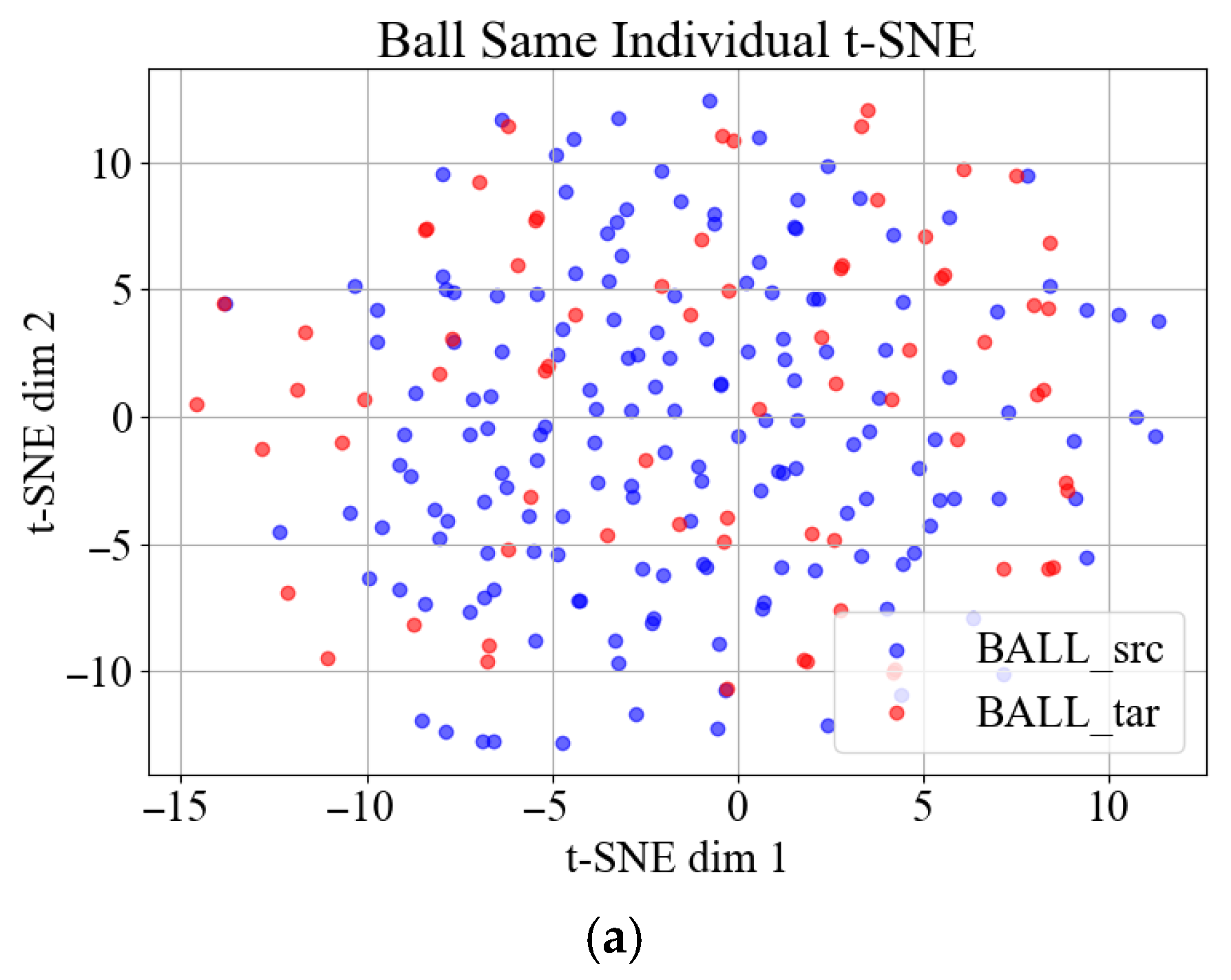
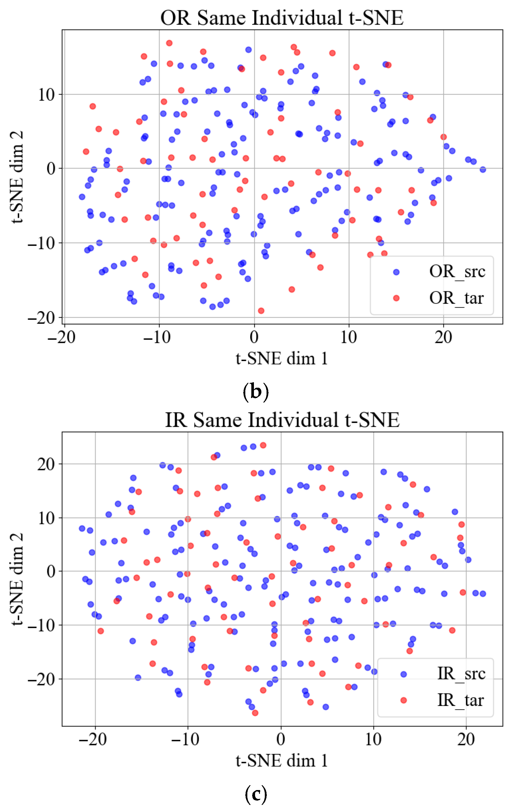
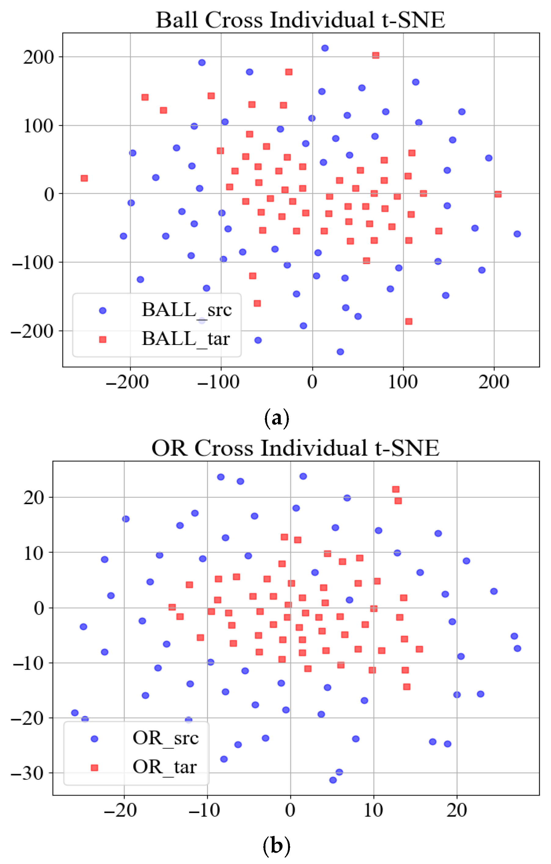
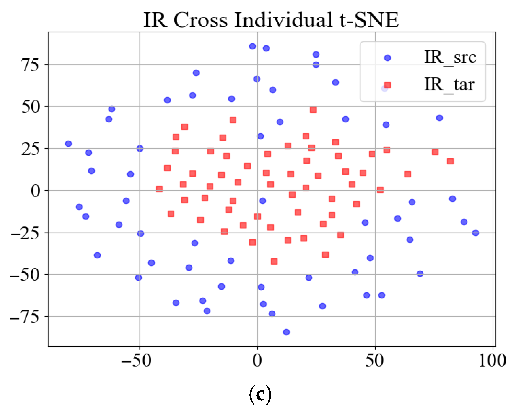
To demonstrate the challenge, the widely cited Case Western Reserve University (CWRU) bearing dataset serves as an illustrative example. Vibration signals corresponding to three distinct bearing fault types, Ball, Inner Race (IR), and Outer Race (OR) from the drive end (DE), were segmented using a sliding window approach to construct the source domain dataset. Respectively, Figure 1a–c and Figure 2a–c present the t-SNE [16] (t-Distributed Stochastic Neighbor Embedding) visualization of the training and testing data distribution for the in-domain task and cross-individual task, where the blue markers represent the dimensionally reduced training set samples and the red markers denote the test set samples in the embedded space.

The t-SNE (t-Distributed Stochastic Neighbor Embedding) visualization reveals the following: (1) compact clustering of same-individual samples (intra-domain consistency), and (2) pronounced distribution shifts between the source (training) and target (testing) individuals, empirically demonstrating the cross-individual generalization challenge in bearing fault diagnosis.

Inspired by the Kolmogorov–Arnold representation theorem (KART) [17], Liu et al. proposed Kolmogorov–Arnold networks (KANs) as promising alternatives to multi-layer perceptrons (MLPs). With a fixed activation function and linear weights replaced by a univariate function parametrized as a spline, KANs tend to show a better nonlinearity expressive capability. This groundbreaking architecture offers promising potential for enhancing model generalization and accuracy. S. Ni et al. [18] applied KANs to sEMG signal classification and achieved exceptionally high accuracy on three datasets, while Cheon et al. [19] employed KANs in remote sensing to improve both efficiency and performance in RS applications. Building on these advancements, KANs hold promise for bearing fault diagnosis based on vibration signals. Considering that not all segments of the spectrum contribute equally to the fault characteristics [20] and the inherent periodicity of vibration signal data, convolution operations and attention mechanisms each offer distinct advantages. The translational invariance of convolution enables the detection of similar local features at different positions, which is crucial for capturing periodic patterns in vibration signals. On the other hand, the attention mechanism, by weighing based on contextual information, captures long-range dependencies and important global information. 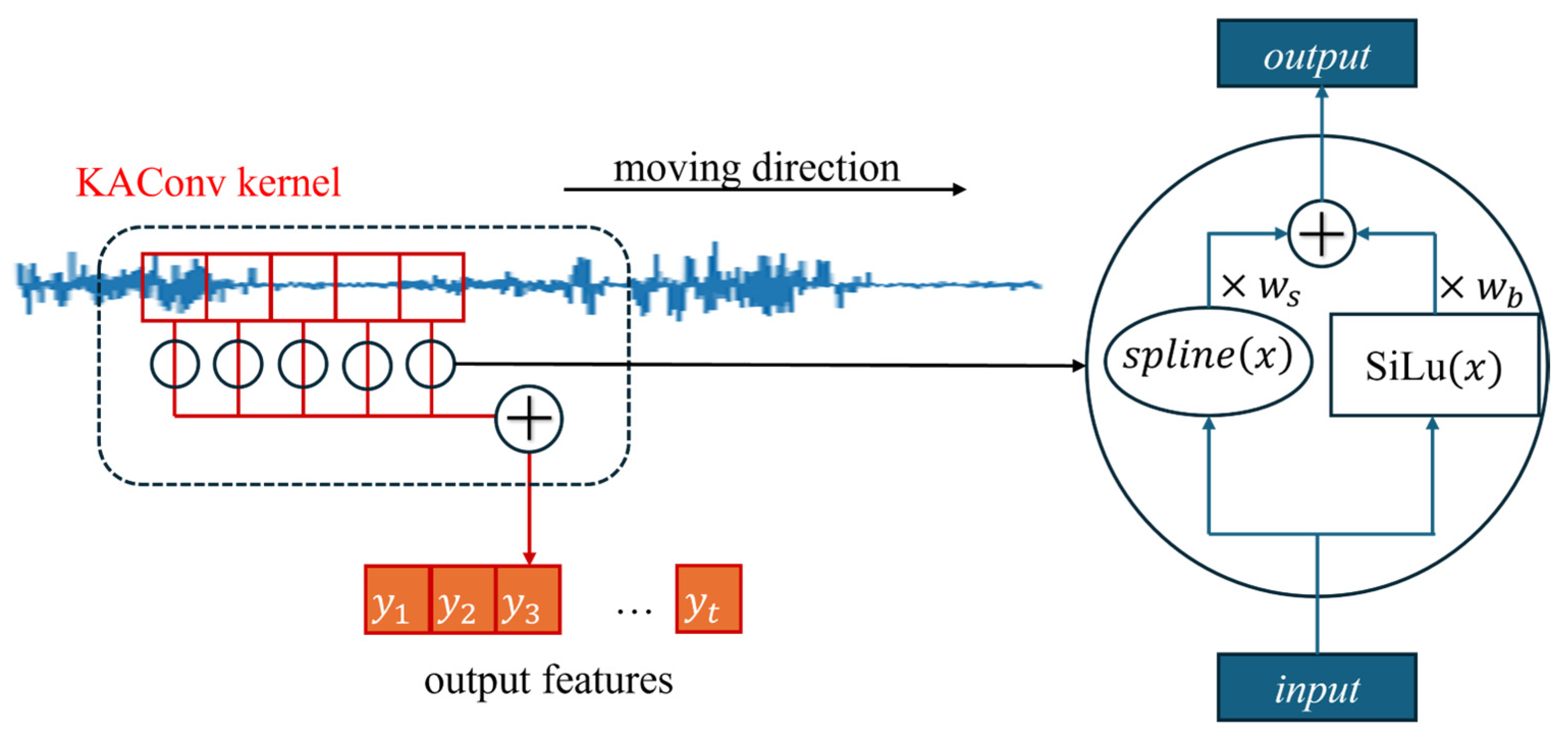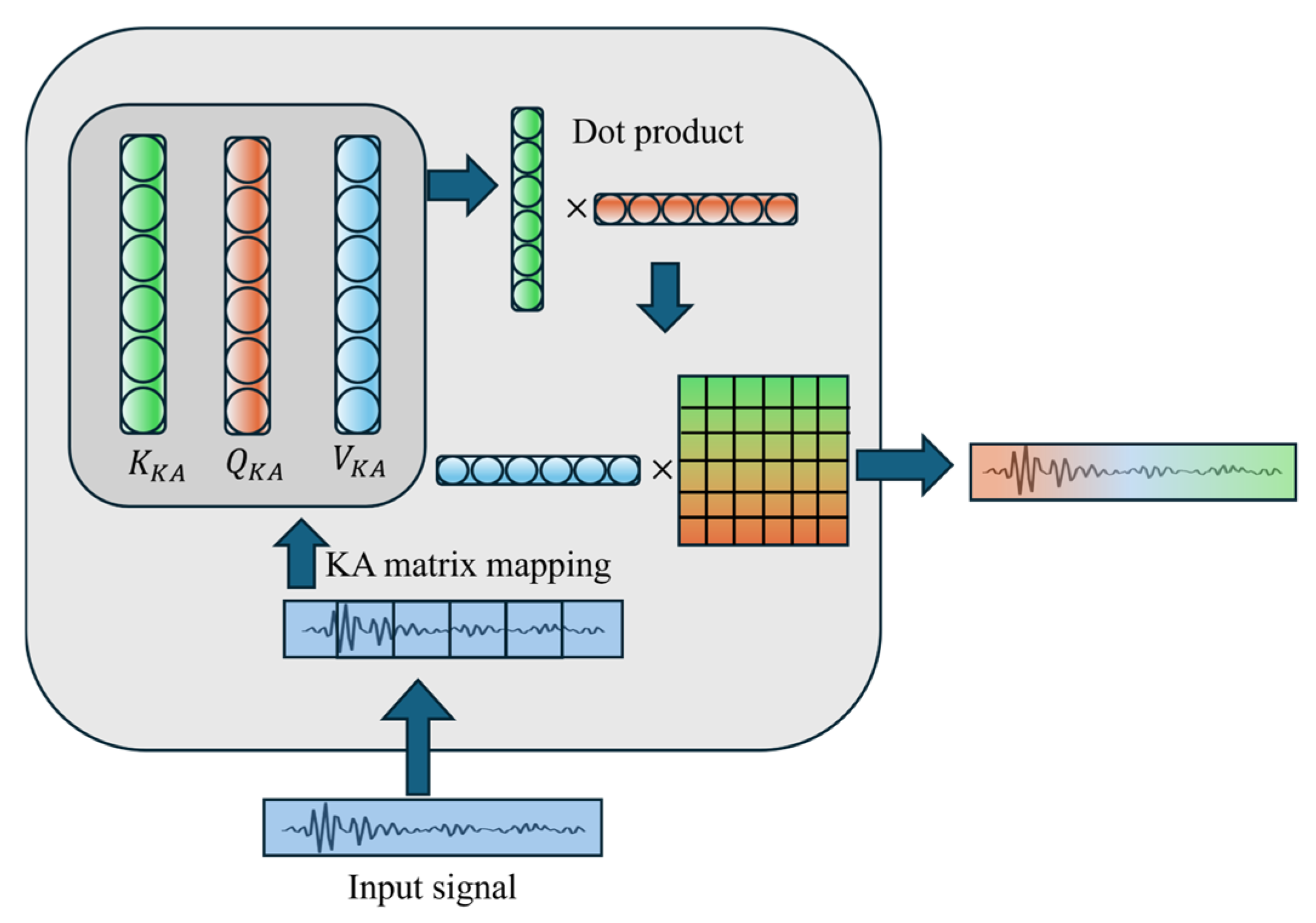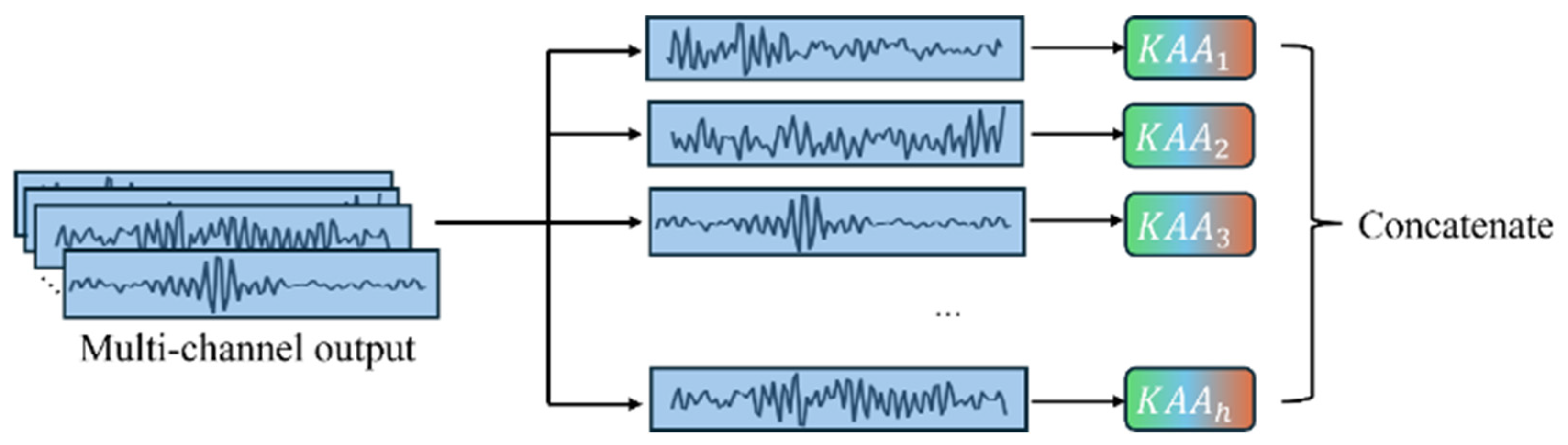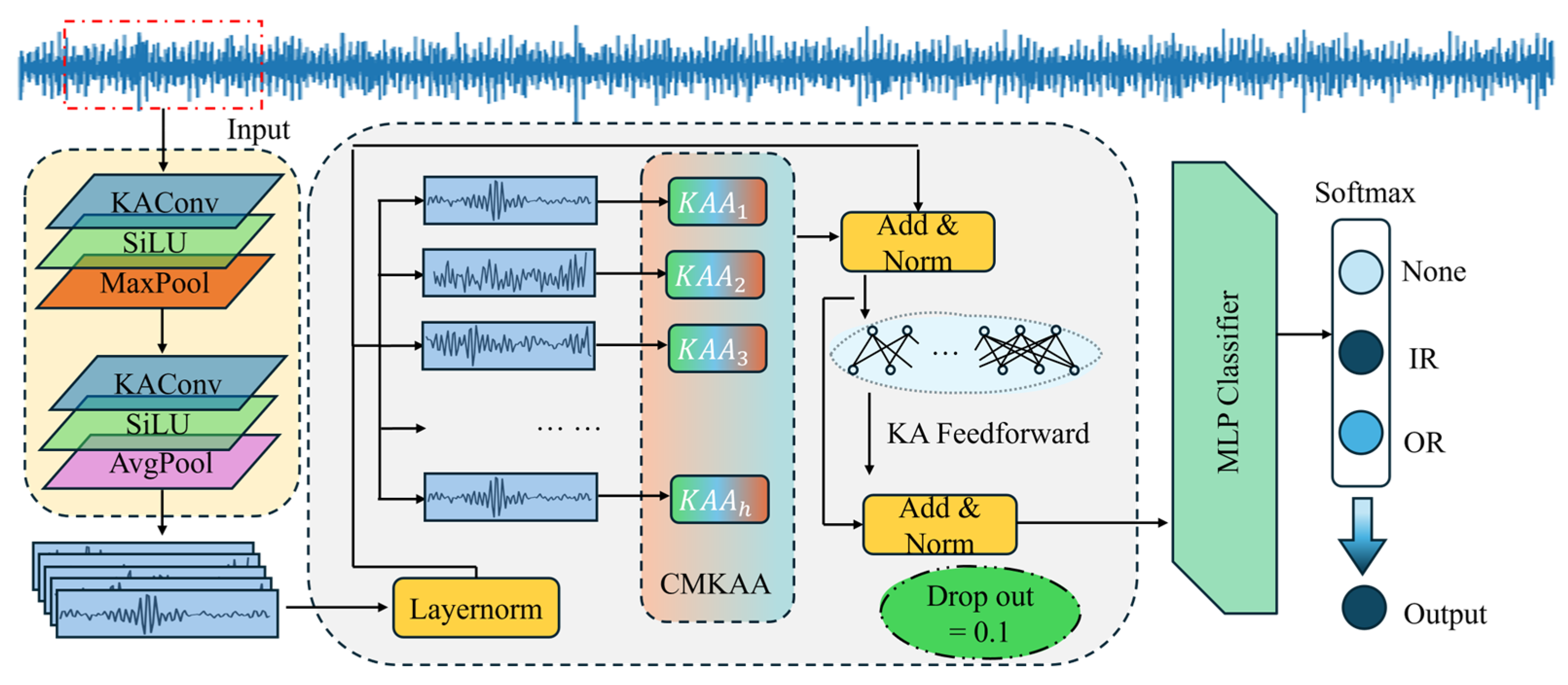So far, the architecture of combining CNN and Transformer has achieved remarkable progress in the field of fault diagnosis to enhance diagnostic accuracy and robustness [21,22]. Therefore, we consider integrating KART into classic CNN and Self-attention modules, proposing two novel modules, KAConv and KAA. This aims to improve the model’s capacity to learn fault types by boosting its ability to capture nonlinear features. The main contributions of this paper are as follows:

(1)

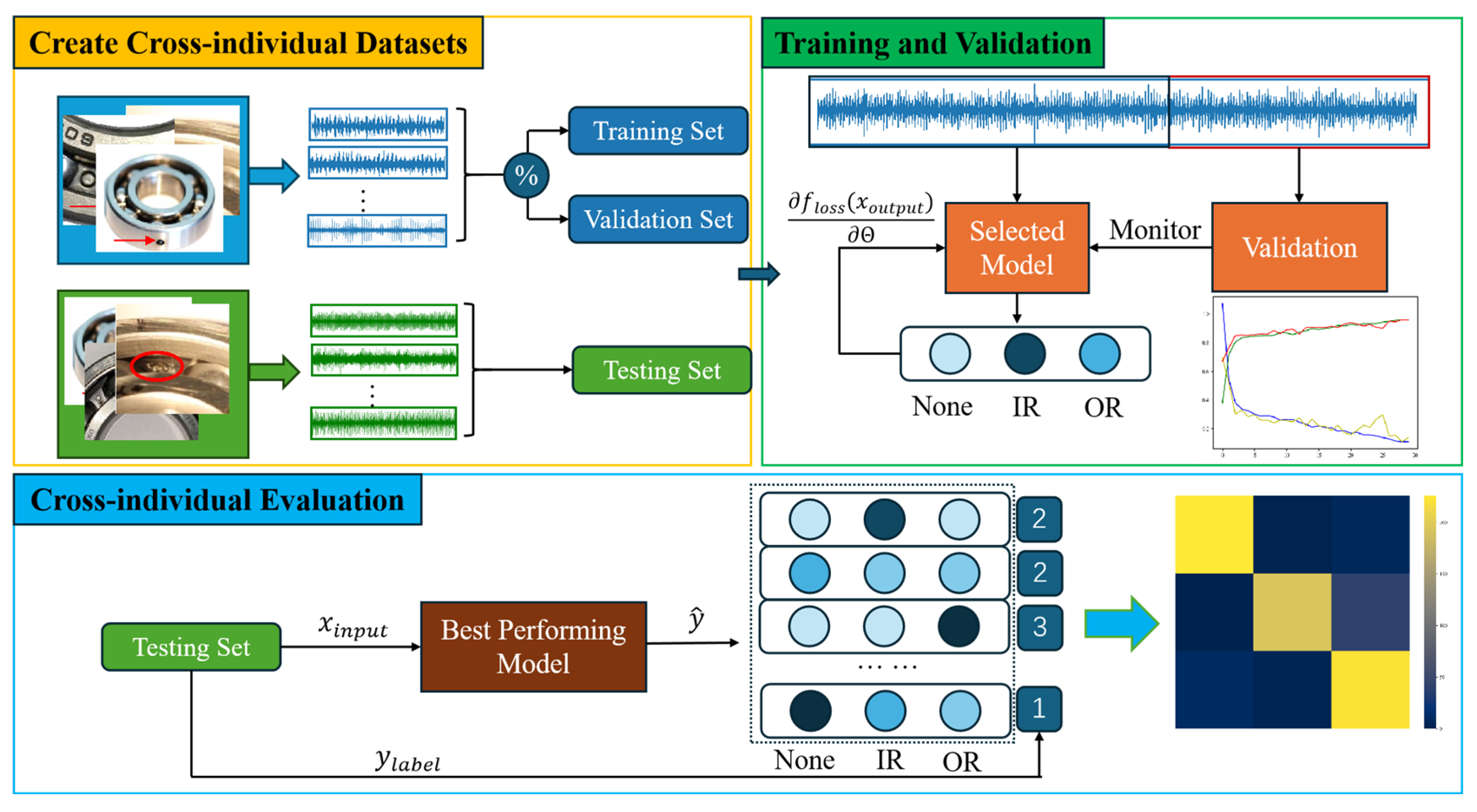
Cross-individual scenarios are explored to provide a reasonable evaluation framework. Under this benchmark, models’ cross-individual generalization capability in real-world scenarios is effectively evaluated.

(2)

A novel Kolmogorov–Arnold enhanced convolutional transformer (KACFormer) model is proposed, which is inspired by KART. KAConv and KAA are designed to improve both general feature representation and cross-individual capabilities.

(3)

Comprehensive comparative experiments are conducted on two public datasets, and experiment results demonstrate the effectiveness and superiority of the proposed method.

The structure of this paper is as follows: Section 2 introduces the method proposed in this paper. Section 3 carries on the experiment and analysis from different aspects. Section 4 gives the main conclusion.

2. Proposed Methods

2.1. Problem Definition

This study focuses on addressing the challenge of cross-individual bearing fault diagnosis by developing a deep learning model capable of recognizing variable fault classes. The primary objective is to train the model using labelled vibration signal data from a diverse set of bearing instances. To be specific, the bearing set used for training $S_{training}$ comprises bearing instances $n_1,n_2,\cdots n_{t1}$, whereas the test bearing set $S_{test}$ consists of bearing instances $m_1,m_2,\cdots m_{t2}$. It is ensured that the intersection of these two sets is an empty set, i.e.,$S_{training} \cap S_{test}=\varnothing$. Simultaneously, the sets of fault classes in both the training and test bearing datasets fully overlap and are drawn from the same fault set $C_f=\left\{1,2,\cdots ,n_{fault}\right\}$, where $n_{fault}$ represents the total number of fault categories. From the two sets of bearing instances described above, the training set and the test set are constructed as follows:

$${\mathit{D}}_{\mathit{t}\mathit{r}\mathit{a}\mathit{i}\mathit{n}}=\left\{\left({\mathit{x}}_{\mathit{i}}^{\left(\mathit{t}\mathit{r}\mathit{a}\mathit{i}\mathit{n}\right)},{\mathit{y}}_{\mathit{i}}^{\left(\mathit{t}\mathit{r}\mathit{a}\mathit{i}\mathit{n}\right)}\right)\right|\mathit{i}=\mathbf{1},\mathbf{2},\cdots ,{\mathit{N}}_{\mathit{t}\mathit{r}\mathit{a}\mathit{i}\mathit{n}}\},$$

(1)

$${\mathit{D}}_{\mathit{t}\mathit{e}\mathit{s}\mathit{t}}=\left\{\left({\mathit{x}}_{\mathit{i}}^{\left(\mathit{t}\mathit{e}\mathit{s}\mathit{t}\right)},{\mathit{y}}_{\mathit{i}}^{\left(\mathit{t}\mathit{e}\mathit{s}\mathit{t}\right)}\right)\right|\mathit{i}=\mathbf{1},\mathbf{2},\cdots ,{\mathit{N}}_{\mathit{t}\mathit{e}\mathit{s}\mathit{t}}\},$$

(2)

where $\forall {\mathit{y}}_{\mathit{i}}^{\left(\mathit{t}\mathit{r}\mathit{a}\mathit{i}\mathit{n}\right)},{\mathit{y}}_{\mathit{i}}^{\left(\mathit{t}\mathit{e}\mathit{s}\mathit{t}\right)}\in {\mathit{C}}_{\mathit{f}}$. Each ${\mathit{x}}_{\mathit{i}}^{\left(\mathit{t}\mathit{r}\mathit{a}\mathit{i}\mathit{n}\right)}$ and ${\mathit{x}}_{\mathit{i}}^{\left(\mathit{t}\mathit{e}\mathit{s}\mathit{t}\right)}$ is an ${\mathit{l}}_{\mathit{s}\mathit{e}\mathit{q}}$-dimensional vibration signal vector, i.e.,${\mathit{x}}_{\mathit{i}}^{\left(\mathit{t}\mathit{r}\mathit{a}\mathit{i}\mathit{n}\right)},{\mathit{x}}_{\mathit{i}}^{\left(\mathit{t}\mathit{e}\mathit{s}\mathit{t}\right)}\in {\mathbb{R}}^{{\mathit{l}}_{\mathit{s}\mathit{e}\mathit{q}}}$. Let the model be a function $\mathit{F}\left(\mathit{x};\mathsf{\Theta }\right):{\mathbb{R}}^{{\mathit{l}}_{\mathit{s}\mathit{e}\mathit{q}}}\to {\mathit{C}}_{\mathit{f}}$, where $\mathsf{\Theta }$ denotes the set of trainable parameters. The key objective is to determine the parameter set $\mathsf{\Theta }$ that maximizes the classification accuracy on ${\mathit{D}}_{\mathit{t}\mathit{e}\mathit{s}\mathit{t}}$. The accuracy on the test set can be defined as

$$\mathit{A}\left({\mathit{D}}_{\mathit{t}\mathit{e}\mathit{s}\mathit{t}};\mathit{\Theta }\right)={\displaystyle \frac{1}{{\mathit{N}}_{\mathit{t}\mathit{e}\mathit{s}\mathit{t}}}}\sum _{\mathit{j}=1}^{{\mathit{N}}_{\mathit{t}\mathit{e}\mathit{s}\mathit{t}}}\mathbb{I}(\mathit{F}\left(\mathit{x};\mathit{\Theta }\right)={\mathit{y}}_{\mathit{i}}^{\left(\mathit{t}\mathit{e}\mathit{s}\mathit{t}\right)}),$$

(3)

where $\mathbb{I}\left(·\right)$ is the indicator function, which is defined as follows:

$$\mathbb{I}\left(\mathit{F}\left(\mathit{x};\mathsf{\Theta }\right)={\mathit{y}}_{\mathit{i}}^{\left(\mathit{t}\mathit{e}\mathit{s}\mathit{t}\right)}\right)=\left\{\begin{array}{c}1, if F\left(\mathit{x};\mathsf{\Theta }\right)={\mathit{y}}_{\mathit{i}}^{\left(\mathit{t}\mathit{e}\mathit{s}\mathit{t}\right)}\\ 0, if F\left(\mathit{x};\mathsf{\Theta }\right)\ne {\mathit{y}}_{\mathit{i}}^{\left(\mathit{t}\mathit{e}\mathit{s}\mathit{t}\right)}\end{array}\right.$$

(4)

The optimization problem could be formulated as follows:

$${\mathsf{\Theta }}^{\mathbf{*}}=\mathbf{arg}\underset{\mathsf{\Theta }}{\mathbf{max}}\mathit{A}\left({\mathit{D}}_{\mathit{t}\mathit{e}\mathit{s}\mathit{t}};\mathsf{\Theta }\right).$$

(5)

This formulation ensures the model achieves reliable fault detection and diagnosis for the bearing individuals in the target set.

2.2. Overall Framework

As shown in Figure 3, the overall framework of our work is divided into three parts: data processing and dataset creation, model training and training process monitoring, and model testing and performance evaluation.

(1)

The task sets are constructed following the methodology in Section 2.1. The validation set is obtained by sampling a specific proportion from the source domain data, ensuring no overlap with the training set.

(2)

The KACFormer model is trained for ${\mathit{n}}_{\mathit{n}\mathit{u}\mathit{m}\_\mathit{e}\mathit{p}\mathit{o}\mathit{c}\mathit{h}}$ on the training set. At the end of each epoch, the model is evaluated with the validation set. Notably, target individuals remain unseen by the model throughout the training process. Additionally, only the model that achieves the highest accuracy on the validation set will be saved.

(3)

After training for ${\mathit{n}}_{\mathit{n}\mathit{u}\mathit{m}\_\mathit{e}\mathit{p}\mathit{o}\mathit{c}\mathit{h}}$ epochs, the best-performing model is tested on the test set made from distinct individuals. Cross-individual accuracy and confusion metrics are utilized to assess the model’s performance.

2.3. Proposed Modules

2.3.1. 1D-KAConv

Convolutional computation provides translational invariance, enabling the detection of similar patterns regardless of their position in the sequence [23]. Additionally, its local receptive fields facilitate the effective extraction of short-term patterns, peaks, and transient events. However, despite these strengths, conventional convolutional filters are fundamentally linear operators, limiting their ability to capture the intricate nonlinear relationships that are inherent in complex time-series data. This shortfall can hamper the model’s overall representational power when dealing with signals exhibiting nonstationary characteristics. The success of prior works motivates our integration of nonlinear mappings within the Kanlinear module [24]. The incorporation of the Kanlinear computational module effectively addresses the limitations of linear convolutional layers in modeling nonlinear relationships, thereby enhancing the model’s suitability for complex cross-individual tasks. The KAConv kernel is the essence of the KAConv module. Figure 4 shows the computation process.

Considering the optimizability of KANs, an integrated neuron connected by residual activation, the Kanlinear unit, is designed. Given an input x, the output of the Kanlinear unit is the weighted sum of a trainable spline function and a fixed activation function,

$$\mathit{\varphi }\left(\mathit{x}\right)={\mathit{w}}_{\mathit{b}}\mathit{b}\left(\mathit{x}\right)+{\mathit{w}}_{\mathit{s}}\mathit{s}\mathit{p}\mathit{l}\mathit{i}\mathit{n}\mathit{e}\left(\mathit{x}\right),$$

(6)

where $w_b$ and $w_s$ are weighs of corresponding residual branch. To be specific, the $b\left(x\right)$ here is a $SiLU\left(x\right)$ function:

$$\mathit{b}\left(\mathit{x}\right)=\mathit{S}\mathit{i}\mathit{L}\mathit{U}\left(\mathit{x}\right)={\displaystyle \frac{\mathit{x}}{1+{\mathit{e}}^{-\mathit{x}}}}.$$

(7)

This unique kernel processes relationships within the receptive field and progressively maps the initial signals to a lower dimensional KA feature space. The outputs of step $t$ of a KAConv kernel with a size of $K$ can be formulated as

$${\mathit{y}}_{\mathit{t}}=\sum _{\mathit{i}=0}^{\mathit{K}}({\mathit{w}}_{\mathit{t}+\mathit{i}}^{\mathit{b}}\mathit{S}\mathit{i}\mathit{L}\mathit{U}\left({\mathit{x}}_{\mathit{t}+\mathit{i}}\right)+{\mathit{w}}_{\mathit{t}+\mathit{i}}^{\mathit{s}}\mathit{s}\mathit{p}\mathit{l}\mathit{i}\mathit{n}\mathit{e}\left({\mathit{x}}_{\mathit{t}+\mathit{i}}\right))$$

(8)

where $x_{t+i}$ is the input signal at time $(t+i)$, $w_{t+i}^b$ is the weight for the $SiLU\left(x\right)$ part at position $i$ of the kernel, and $w_{t+i}^s$ is the weight for the $spline\left(x_{t+i}\right)$ part at position $i$ of the kernel. Based on this, we define the 1D multi-channel KAConv operation as

$${\mathbf{K}\mathbf{A}\mathbf{C}\mathbf{o}\mathbf{n}\mathbf{v}\left(\mathbf{X}\right):\mathbb{R}}^{{{\mathit{n}}_1\times \mathit{l}}_1}\to {\mathbb{R}}^{{{\mathit{n}}_2\times \mathit{l}}_2}$$

(9)

where $n1$ and $l1$ are the number of channels and the sequence length of the input data, respectively, while $n2$ and $l2$ correspond to the number of channels and the sequence length of the output feature.

2.3.2. Channel-Wise Multihead KAA

Multi-Head Self-attention mechanism is a key defining characteristic of transformer models [25]. The Self-attention mechanism captures global dependencies within data, enabling each element in a sequence to interact with all others, which ensures the comprehensive understanding and integration of context across the entire sequence. By mapping input signals into a space with the same dimension, the KA-Attention (KAA) mechanism enhances the model’s nonlinear expressive power, empowering models to uncover and leverage complex patterns, which is shown in Figure 5.

Given an input sequence represented by a matrix $X\in {\mathbb{R}}^{n\times d}$, where $n$ is the sequence length and $d$ is the dimensionality of each input vector, the KAA mechanism computes three distinct matrixes: KAQueries ($Q_{KA}$), KAKeys ($K_{KA}$), and KAValues ($V_{KA}$). These matrixes are derived through learned linear transformations of the input:

$${\mathit{Q}}_{\mathit{K}\mathit{A}}=\mathit{X}{\mathit{W}}_{{\mathit{Q}}_{\mathit{K}\mathit{A}}},$$

(10)

$${\mathit{K}}_{\mathit{K}\mathit{A}}=\mathit{X}{\mathit{W}}_{{\mathit{K}}_{\mathit{K}\mathit{A}}},$$

(11)

$${\mathit{V}}_{\mathit{K}\mathit{A}}=\mathit{X}{\mathit{W}}_{{\mathit{V}}_{\mathit{K}\mathit{A}}},$$

(12)

where $W_{Q_{KA}}\in {\mathbb{R}}^{d\times d_k}$, $W_{K_{KA}}\in {\mathbb{R}}^{d\times d_k}$, and $W_{V_{KA}}\in {\mathbb{R}}^{d\times d_V}$ are learnable Kanlinear matrixes for $Q_{KA}$, $K_{KA}$, and $V_{KA}$, respectively. To be specific, they can be formulated as matrixes:

$${\mathit{W}}_{{\mathit{Q}}_{\mathit{K}\mathit{A}}}=\left[\begin{array}{ccc}{\mathit{\varphi }}_{11}^{\mathit{q}}& \cdots & {\mathit{\varphi }}_{1{\mathit{d}}_{\mathit{k}}}^{\mathit{q}}\\ ⋮& \ddots & ⋮\\ {\mathit{\varphi }}_{\mathit{d}1}^{\mathit{q}}& \cdots & {\mathit{\varphi }}_{\mathit{d}{\mathit{d}}_{\mathit{k}}}^{\mathit{q}}\end{array}\right],$$

(13)

$${\mathit{W}}_{{\mathit{K}}_{\mathit{K}\mathit{A}}}=\left[\begin{array}{ccc}{\mathit{\varphi }}_{11}^{\mathit{k}}& \cdots & {\mathit{\varphi }}_{1{\mathit{d}}_{\mathit{k}}}^{\mathit{k}}\\ ⋮& \ddots & ⋮\\ {\mathit{\varphi }}_{\mathit{d}1}^{\mathit{k}}& \cdots & {\mathit{\varphi }}_{\mathit{d}{\mathit{d}}_{\mathit{k}}}^{\mathit{k}}\end{array}\right],$$

(14)

$${\mathit{W}}_{{\mathit{V}}_{\mathit{K}\mathit{A}}}=\left[\begin{array}{ccc}{\mathit{\varphi }}_{11}^{\mathit{v}}& \cdots & {\mathit{\varphi }}_{1{\mathit{d}}_{\mathit{k}}}^{\mathit{v}}\\ ⋮& \ddots & ⋮\\ {\mathit{\varphi }}_{\mathit{d}1}^{\mathit{v}}& \cdots & {\mathit{\varphi }}_{\mathit{d}{\mathit{d}}_{\mathit{k}}}^{\mathit{v}}\end{array}\right],$$

(15)

where each $\varphi$ is a learnable Kanlinear unit. Once $Q_{KA}$, $K_{KA}$, and $V_{KA}$ are computed, the KAA mechanism calculates the attention scores:

$$\mathit{K}\mathit{A}\mathit{A}\left({\mathit{Q}}_{\mathit{K}\mathit{A}},{\mathit{K}}_{\mathit{K}\mathit{A}},{\mathit{V}}_{\mathit{K}\mathit{A}}\right)=\mathit{s}\mathit{o}\mathit{f}\mathit{t}\mathit{m}\mathit{a}\mathit{x}\left({\displaystyle \frac{{\mathit{Q}}_{\mathit{K}\mathit{A}}{{\mathit{K}}_{\mathit{K}\mathit{A}}}^{\mathit{T}}}{\sqrt{{\mathit{d}}_{\mathit{k}}}}}\right){\mathit{V}}_{\mathit{K}\mathit{A}},$$

(16)

where the softmax function ensures that the attention weights are normalized, facilitating a weighted aggregation of the values $V_{KA}$ based on their relevance to each query $Q_{KA}$.

Through the feature extraction operations of the preceding KAConv layers, the input signal is transformed into multi-channel data. To capture and optimize the distinct characters of each channel, the channel-wise multi-head KAA (CMKAA) is designed. Signals from each channel are assigned to different KAA heads. The outputs of each head are concatenated, which is shown in Figure 6. Formally, this process can be formulated as

$$\mathit{C}\mathit{M}\mathit{K}\mathit{A}\mathit{A}\left(\mathit{X}\right)=\mathit{C}\mathit{o}\mathit{n}\mathit{c}\mathit{a}\mathit{t}\left({\mathit{K}\mathit{A}\mathit{A}}_1\left({\mathit{x}}_1\right),\cdots {\mathit{K}\mathit{A}\mathit{A}}_{\mathit{h}}\left({\mathit{x}}_{\mathit{h}}\right)\right),$$

(17)

where $x_i$ is the output sequence of the $i$th channel and $h$ is the number of heads.

2.4. KACFormer Model

The overall structure of the KACFormer model is illustrated in Figure 7. Initially, the input signal is encoded into multi-channel features with the KAConv Encoder. The encoder consists of two KAConv Blocks. Each block is equipped with a KAConv layer, a SiLU activation layer, and a pooling layer. Note that the normalizing operation is dropped intentionally. According to the relevant literature, large vibration amplitudes are indicative of bearing faults [19]. Therefore, a maxpooling layer is employed in the first KAConv Block to accentuate peak characteristics. To reduce the overfitting risk and the impact of irrelevant high activations caused by noise, an avgpooling layer is employed in the second KAConv Block. The ith KAConv Block computation can be formally written as below:

$$\mathit{B}\mathit{l}\mathit{o}\mathit{c}{\mathit{k}}_{\mathit{K}\mathit{A}\mathit{C}\mathit{o}\mathit{n}\mathit{v}}^{\mathit{i}}\left(\mathit{X}\right)=\mathit{P}\mathit{o}\mathit{o}\mathit{l}\mathit{i}\mathit{n}\mathit{g}\left\{\mathit{S}\mathit{i}\mathit{L}\mathit{U}\left[\mathit{K}\mathit{A}\mathit{C}\mathit{o}\mathit{n}\mathit{v}\left(\mathit{X}\right)\right]\right\}.$$

(18)

Once the row signal is encoded, it is sent into the transformer block. To better align with the KATR, adjustments are made based on the classic transformer architecture by Vaswani, Ashish, et al. [25]. Considering the volume of data, the transformer architecture is designed to be shallow with only one layer to avoid the risks of overfitting, improving its model generalization capacity. Meanwhile, a KA feed-forward (KAFF) layer with SiLU activation is designed, mapping its input to a vector with the same dimension:

$$\mathit{K}\mathit{A}\mathit{F}\mathit{F}\left(\mathit{x}\right)=\mathit{S}\mathit{i}\mathit{L}\mathit{U}\left({\mathit{w}}_{\mathit{b}}\mathit{S}\mathit{i}\mathit{L}\mathit{U}\left(\mathit{x}\right)+{\mathit{w}}_{\mathit{s}}\mathit{s}\mathit{p}\mathit{l}\mathit{i}\mathit{n}\mathit{e}\left(\mathit{x}\right)\right).$$

(19)

The residual structures of the classic transformer are retained to keep the optimizability of the model. Given an input matrix $X^{n_{channel}\times l_{seq}}$, let

$$\mathit{R}\mathit{e}\mathit{s}=\mathit{L}\mathit{a}\mathit{y}\mathit{e}\mathit{r}\mathit{n}\mathit{o}\mathit{r}\mathit{m}(\mathit{C}\mathit{M}\mathit{K}\mathit{A}\mathit{A}\left(\mathit{X}\right)+\mathit{X}),$$

(20)

The output of the CMKAA transformer can be written as follows:

$$\mathit{O}\mathit{u}\mathit{t}\mathit{p}\mathit{u}\mathit{t}=\mathit{L}\mathit{a}\mathit{y}\mathit{e}\mathit{r}\mathit{n}\mathit{o}\mathit{r}\mathit{m}\left(\mathit{K}\mathit{A}\mathit{F}\mathit{F}\left(\mathit{R}\mathit{e}\mathit{s}\right)+\mathit{R}\mathit{e}\mathit{s}\right).$$

(21)

3. Experiments

To validate the effectiveness and the necessity of the proposed modules in the task, comprehensive experiments on two open datasets are conducted, including ablation study and contrast experiments. The code is written in Python 3.10.14 with Pytorch 2.4.1+cu124 on the computer, manufactured by Lenovo in Beijing, China, with an NVIDIA GeForce RTX 4060 Laptop GPU.

3.1. Task Setups

3.1.1. Task 1 on PU Dataset

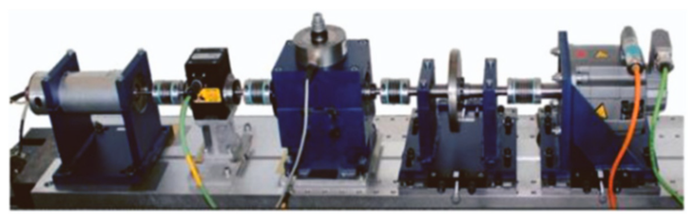
The dataset for the first cross-individual task is sourced from the PU dataset from the Paderborn University Konstruktions und Antriebstechnik (KAt) data center [26]. Vibration signals from the bearing housing are collected using piezoelectric accelerometers at a sampling frequency of 64 kHz. The experimental test platform, including a drive motor, load motor, flywheel, torque sensor, and module for testing bearing vibration data, is shown in Figure 8.

A total of 32 different bearings are included in the PU dataset. These bearings vary in terms of their manufacturer, type, and severity of damage, aligning with the objectives of our cross-individual study. The bearing faults in the dataset are generated using two primary methods: electrical discharge machining (EDM) and life acceleration treatment. To ensure the experiments closely resemble real-world industrial scenarios, only the data obtained through life acceleration treatment is utilized. The fault positions considered in this study include Healthy (N), Outer Race (OR), and Inner Race (IR). Additionally, to avoid an imbalanced dataset, only a subset of the provided bearings is used. The chosen bearings for the training and validation sets are K001 (N), K002 (N), K003 (N), KA04 (OR), KA15 (OR), KA16 (OR), KI04 (IR), KI14 (IR), and KI16 (IR). For the testing sets, we selected K006 (N), KA22 (OR), and KI21 (IR).

All data is collected under the same working conditions, with a rotational speed of 900 rpm, load torque of 0.7 Nm, and radial force of 1000 N. The official working condition code is “N09_M07_F10”. Detailed information about the chosen bearings is provided on

Table 1. Detailed information on the chosen bearings from the PU dataset.

Data Sets	Bearing Code	Manufacturer	Damage	Combination	Arrangement	Extent of Damage	Fault Type	Fault Code
Training sets	K001	IBU	-	-	-	-	N	1
	K002	IBU	-	-	-	-	N	1
	K003	IBU	-	-	-	-	N	1
	KA04	FAG	fatigue: pitting	S	no repetition	1	OR	2
	KA15	FAG	Plastic deforms: Indentations	S	no repetition	1	OR	2
	KA16	MTK	fatigue: pitting	R	random	2	OR	2
	KI04	MTK	fatigue: pitting	M	no repetition	1	IR	3
	KI14	MTK	fatigue: pitting	M	no repetition	1	IR	3
	KI16	FAG	fatigue: pitting	S	no repetition	3	IR	3
Testing sets	K006	IBU	-	-	-	-	N	1
	KA22	IBU/IBB	fatigue: pitting	S	no repetition	1	OR	2
	KI21	FAG	fatigue: pitting	S	no repetition	1	IR	3

.

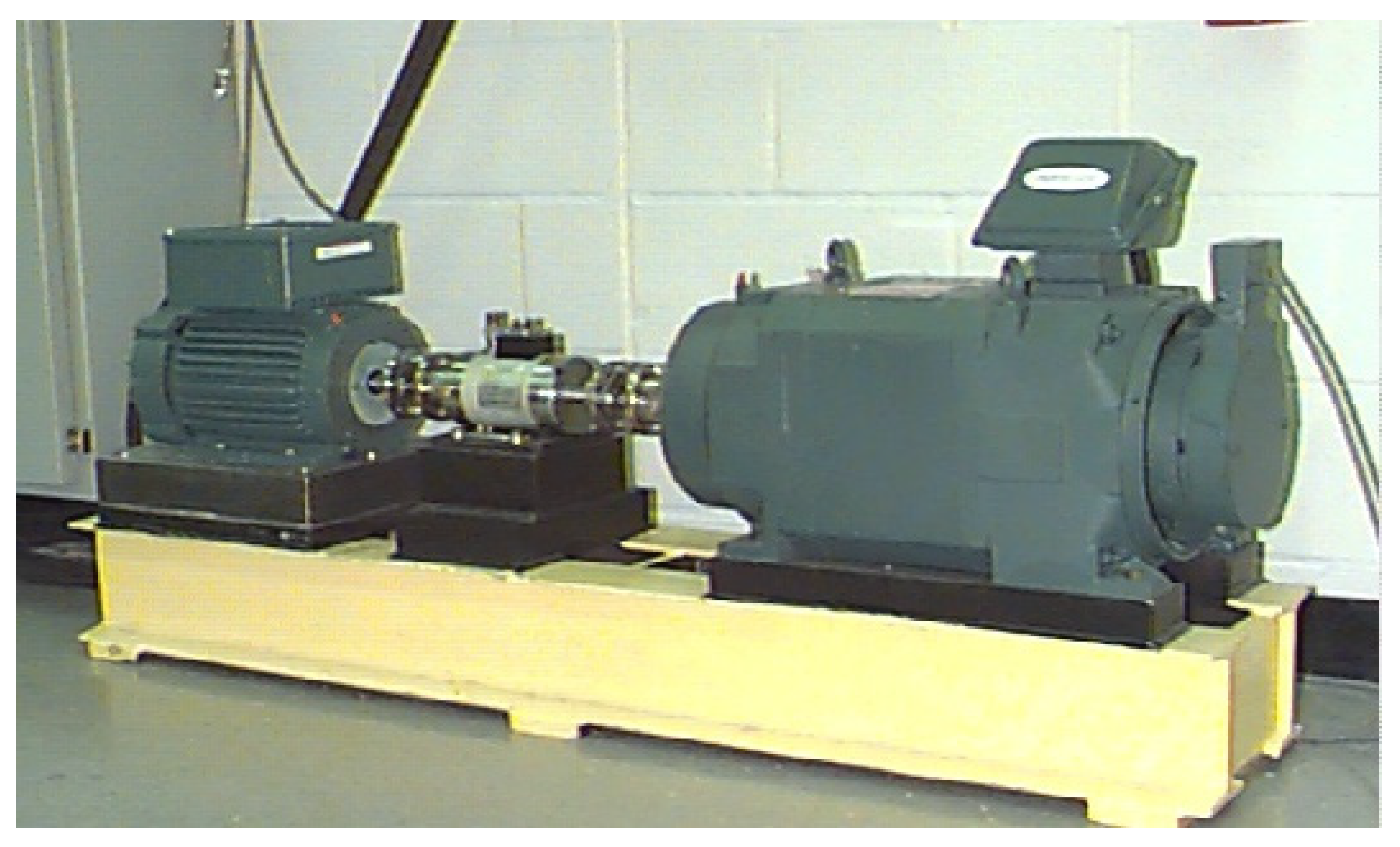
3.1.2. Task 2 on CWRU Dataset

The dataset for Task 2 is derived from the highly cited CWRU dataset [27]. The test bench consists of a 2 HP motor, a torque transducer, and a power dynamometer. The accelerometers are mounted on the drive side and the fan side of the housing to collect vibration signals, as shown in Figure 9.

The CWRU dataset provides two distinct types of bearings for cross-individual task research, namely the drive end (DE) bearing (6205-2RS JEM SKF; deep groove ball bearing) and the fan end (FE) bearing (6203-2RS JEM SKF; deep groove ball bearing). According to official records, the parameters for the two different bearings are listed in

Table 2. Detailed information on the chosen bearings from the CWRU dataset.

Bearing	Inside Diameter	Outside Diameter	Thickness	Ball Diameter	Pitch Diameter
DE	0.9843	2.0472	0.5906	0.3126	1.537
FE	0.6693	1.5748	0.4724	0.2656	1.122

.

The CWRU dataset provides a relatively smaller scale of data for cross-individual fault diagnosis research. According to the relevant literature [28], models tend to face greater challenges in distinguishing fault classes when subjected to higher loads. Regarding the difficulty caused by a relatively insufficient data volume, Task 2 was set on the working condition with 0 HP load. In Task 2, we utilize data collected from the DE bearings to train the model, while data from the FE bearings is used to test the model. Task 2 is also a three-class classification task, including Healthy, OR fault and IR fault.

3.1.3. Other Settings

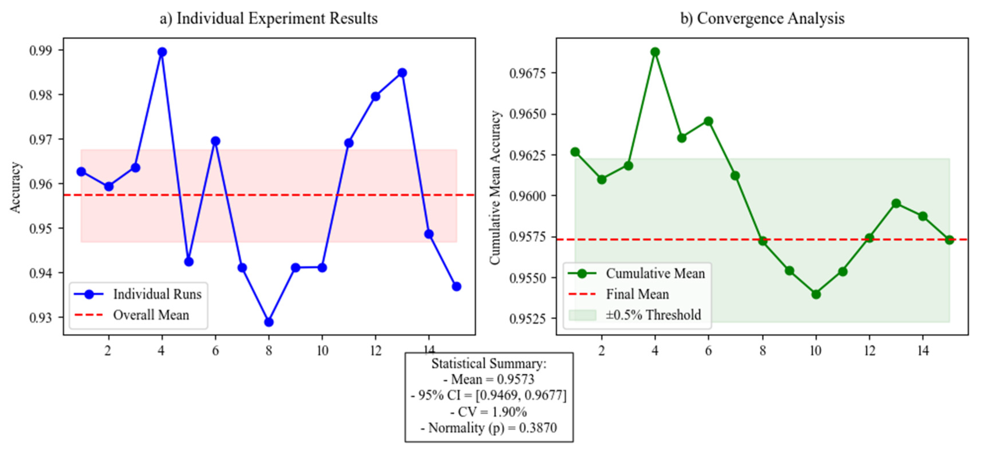
The sliding window has a length of 1024 and an overlapping rate of 0.5. All models are optimized using the Adam optimizer [29] with the learning rate set to 0.001. Cross-entropy is used as the loss function to complete backpropagation and parameter updates for the models. To prevent model overfitting and achieve optimal performance on cross-individual tasks, multiple training runs are performed with different numbers of epochs, and the epoch number that yields the best accuracy on the target bearings is selected. Through experiments, the optimal number of epochs for different models ranges from 5 to 20. Additionally, to avoid the randomness of a single experiment, each model is run 15 times on the same task, and the average performance is taken as the result. The distribution of the training, validation, and testing data for both tasks is presented in

Table 3. Data distribution for both tasks.

	Training		Validation		Testing
Task1	N	1996	N	998	N	998
	IR	2003	IR	1001	IR	998
	OR	2004	OR	1002	OR	998
Task2	N	159	N	79	N	235
	IR	158	IR	79	IR	235
	OR	157	OR	78	OR	236

. As shown in Figure 10, the statistical analysis using Shapiro–Wilk normality testing and confidence interval estimation demonstrates that 15 experimental repetitions yield sufficiently reliable results, with a narrow 95% CI [94.69%, 96.77%] and low variability (CV = 1.90%).

3.2. Model Selection

The hyperparameters of the model are listed in

Table 4. Hyperparameters of the selected model.

Blocks	Layers	Parameters	OUTPUT SHAPE
Input signal	-	-	1 × 2048
KAConv Block1	KAConv	channel = 16, k = 64, s = 16, p = 1	16 × 61
	Activation	SiLU	16 × 61
	MaxPool1D	channel = 16, k = 2, s = 2, p = 0	16 × 30
KAConv Block2	KAConv	channel = 32, k = 2, s = 2, p = 1	32 × 16
	Activation	SiLU	32 × 16
	MaxPool1D	channel = 32, k = 2, s = 2, p = 0	32 × 8
CMKAA Transformer	CMKAA	h = 32, embed dim = 8, dropout = 0.1	32 × 8
	Flatten	-	1 × 256
	KFF	n = 32, activation = SiLU	1 × 256
	Layer norm	-	1 × 256
	Drop out	p = 0.1	1 × 256
MLP classifier	Fc layer1	n = 100, activation = ReLU	1 × 100
	Fc layer2	n = 3, activation = ReLU	1 × 3
	Softmax	-	1 × 3

.

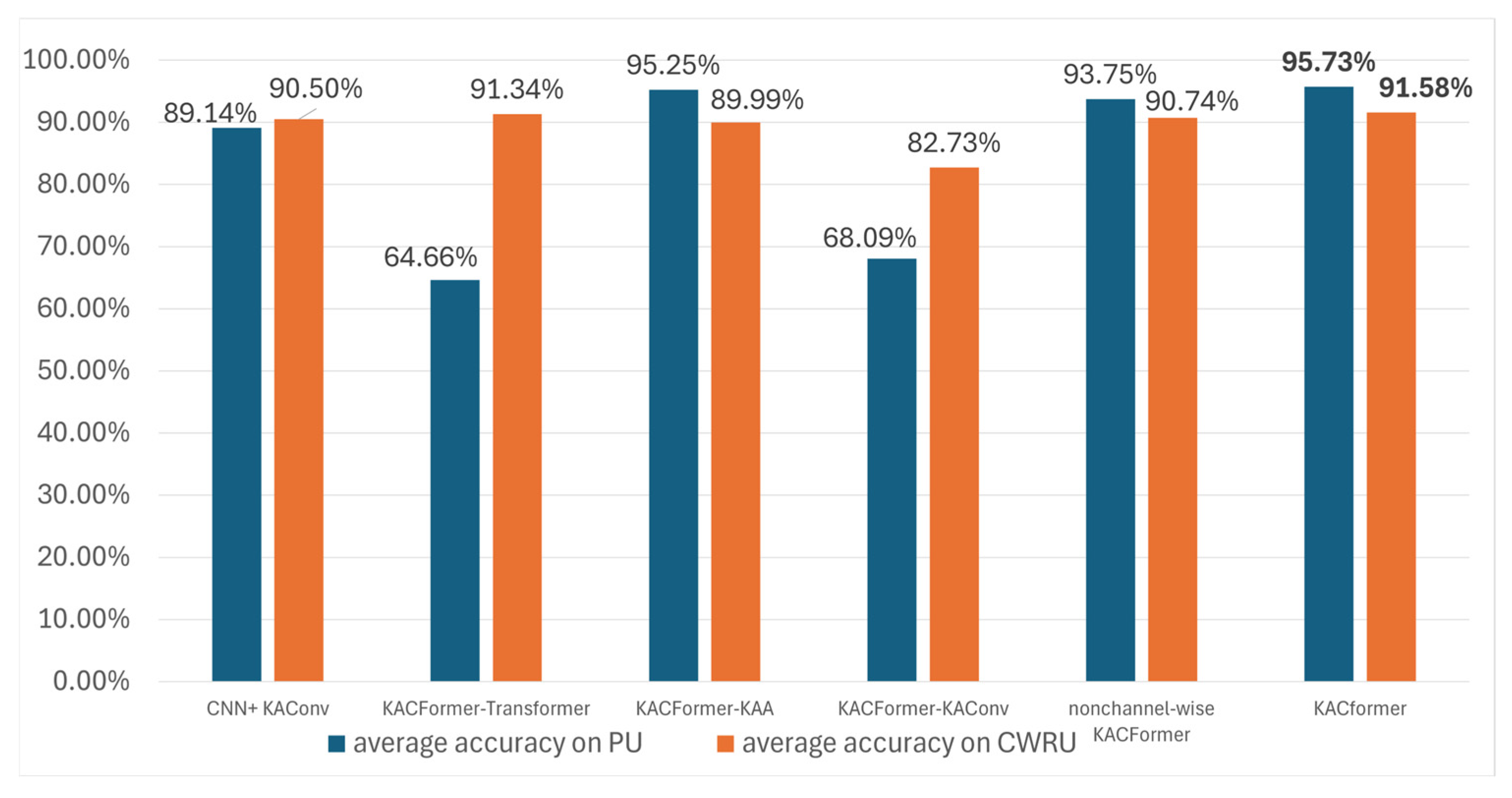
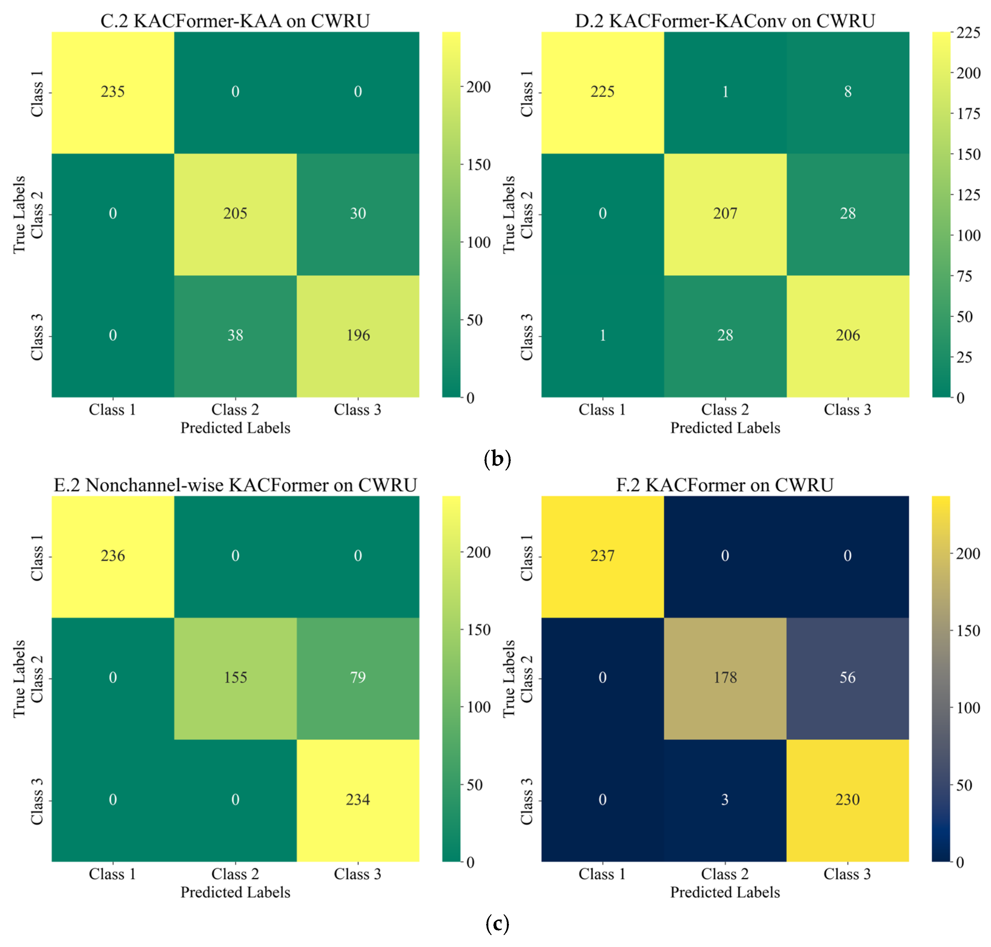
3.3. Ablation Experiment

To evaluate the efficacy of the proposed modules, the ablation experiment is carried out. The models participating in the ablation experiment are as follows:

(A)

CNN+ KAConv. This model has the same structure as the classic WDCNN model. However, all conventional convolution modules are replaced by KAConv modules.

(B)

KACFormer–Transformer. The output of KAConv Encoder is sent directly into the MLP classifier.

(C)

KACFormer–KAA. This model is equipped with the WD-KAConv Encoder, followed by a traditional transformer layer.

(D)

KACFormer–KAConv. Replace the WD-KAConv Encoder with the same structured convolution encoder.

(E)

Non-channel-wise KACFormer (N-KACFormer). Assign more channels to each KAA head.

(F)

KACFormer. The proposed model.

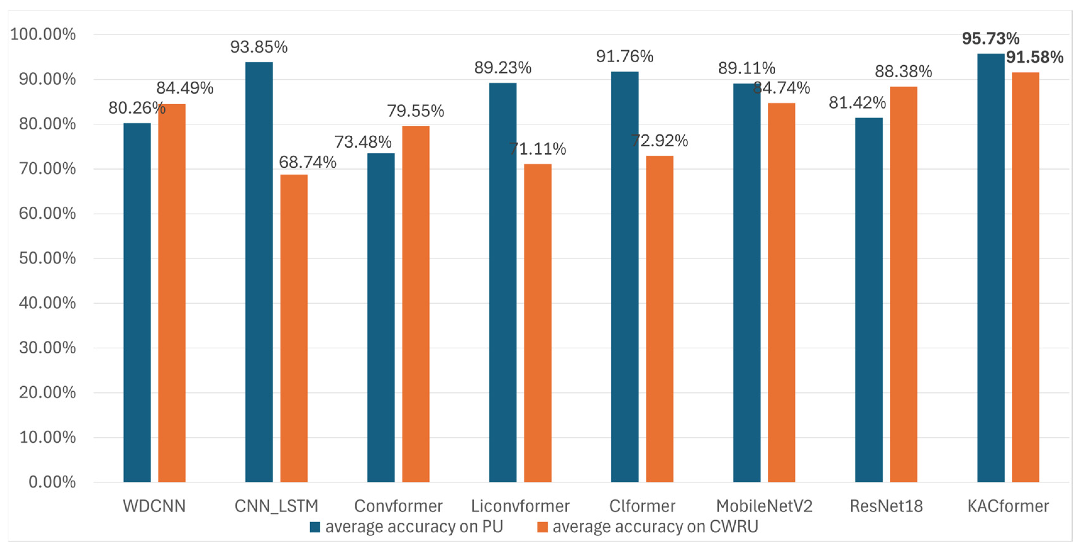
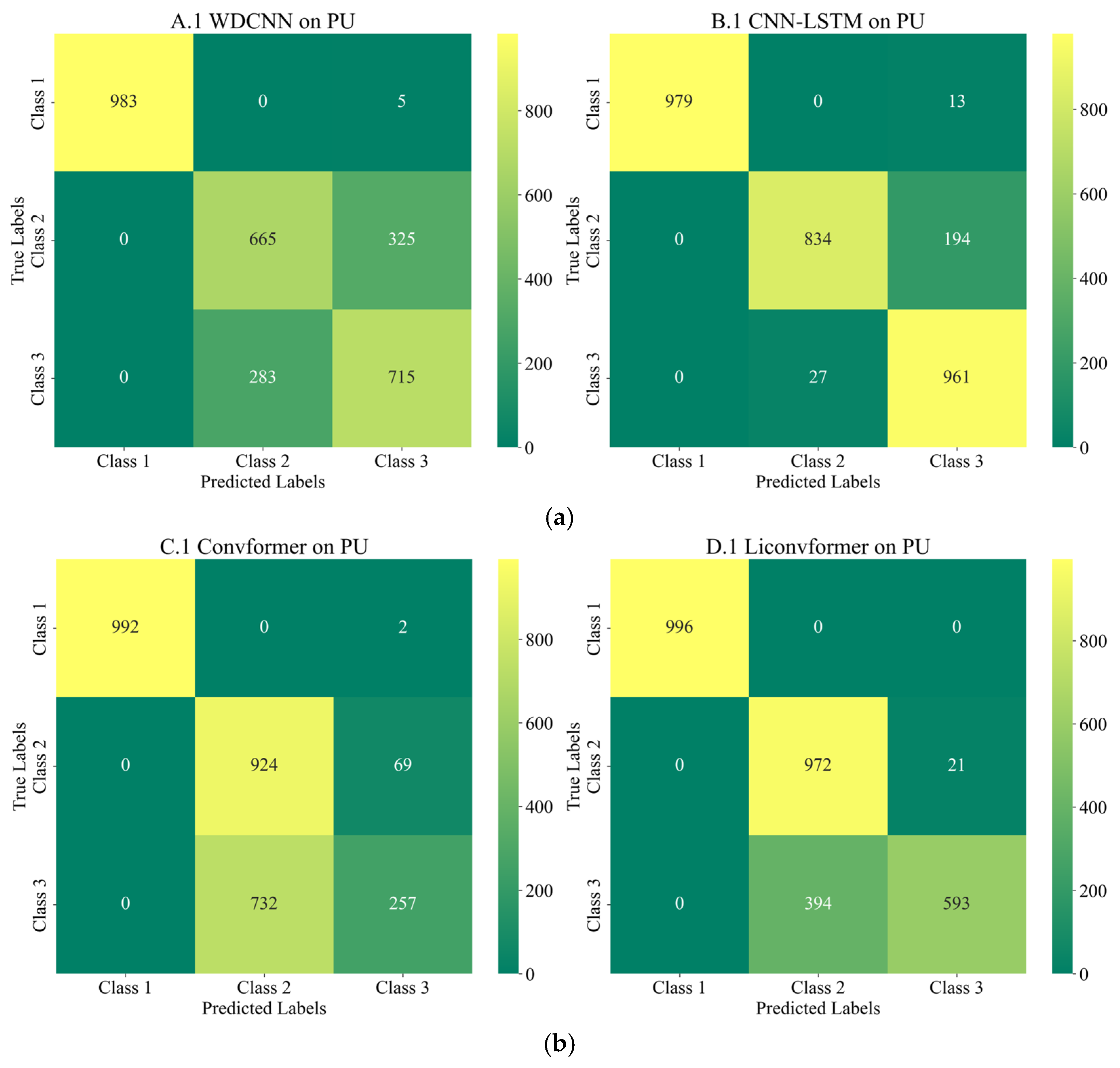
3.4. Contrast Experiment

To validate the advancement of our proposed KACFormer model, we conducted a comprehensive comparative experiment involving both traditional classic models and modern advanced models, ranging from CNN-based methods to contemporary Transformers. The compared models include classic CNN architecture as well as frameworks that share a similar CNN-Transformer structure to our approach. Below are detailed descriptions of the contrasted models:

(A)

WDCNN. Pioneering work in the field of fault diagnosis, serving as the baseline model [6].

(B)

CNN-LSTM. A fault diagnosis model utilizing the CNN module and the LSTM module with 100 neurons set for calculation [30].

(C)

Convformer. A network designed to extract robust features by integrating both global and local information, with the goal of enhancing the end-to-end fault diagnostic performance of gearboxes under high levels of noise [21]. To better adapt to the mission, the small version of the Conformer is utilized.

(D)

Liconvformer. A novel advanced lightweight fault diagnosis model with separable multiscale convolution and broadcast Self-attention [22].

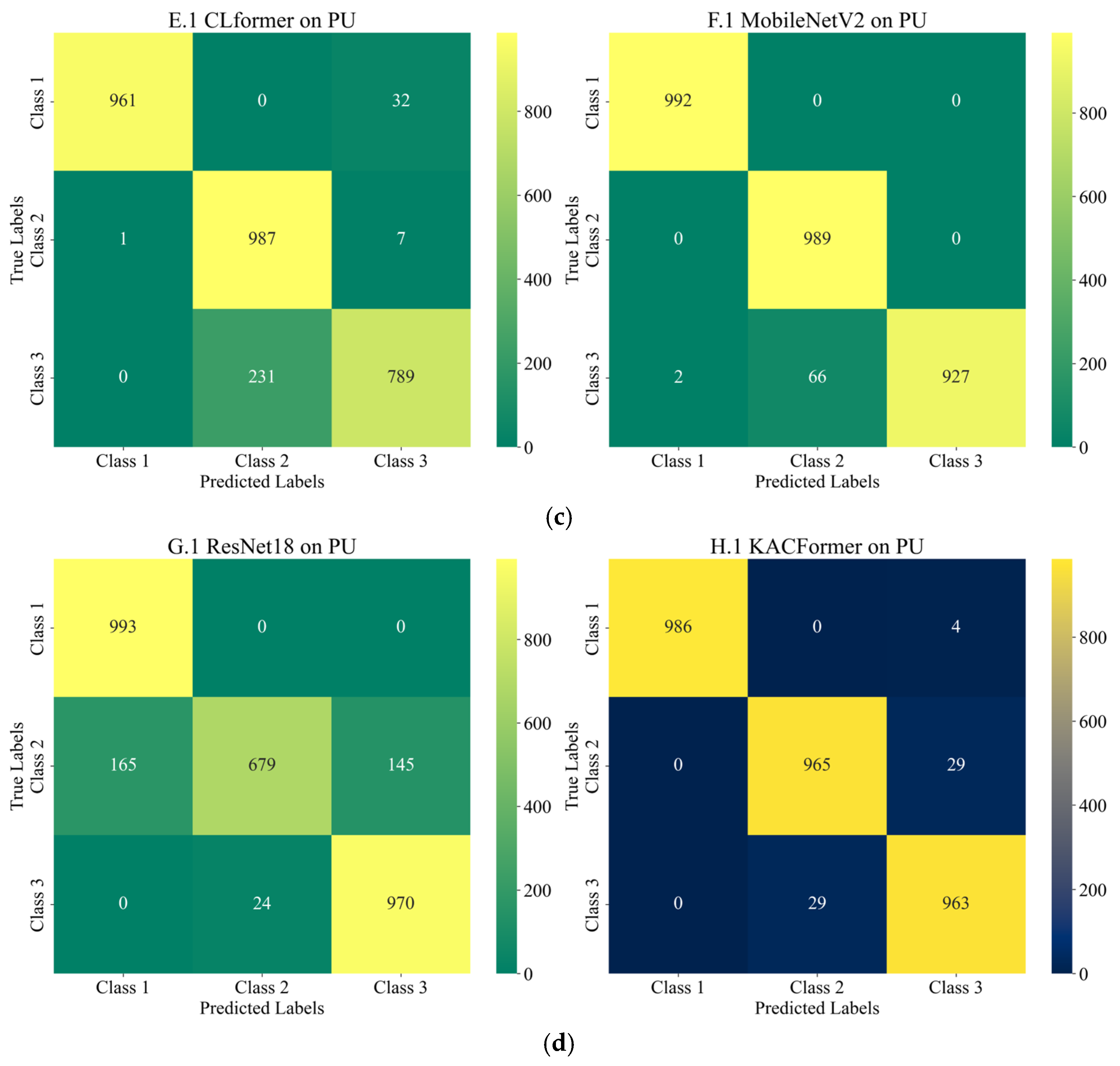
(E)

Clformer. A transformer based on convolutional embedding and Self-Attention mechanisms [31].

(F)

MobileNetV2. This neural network enhances the state-of-the-art performance of mobile models across various tasks, benchmarks, and a wide range of model sizes [32].

(G)

ResNet18. ResNet18 is a convolutional neural network architecture known for its use of residual connections, enabling efficient training of deeper models while maintaining strong performance in image classification and other computer vision tasks [33].

(H)

KACFormer. The proposed model.

3.5. Results and Analysis

3.5.1. Ablation Results

The ablation results are listed in

Table 5. Ablation results.

Task	CNN+ KAConv	KACFormer-Transformer	KACFormer-KAA	KACFormer-KAConv.	N-KACFormer	KAC-Former
PU	89.14%	64.66%	95.25%	68.09%	93.75%	95.73%
CWRU	90.50%	91.34%	89.99%	82.73%	90.74%	91.58%

and Figure 11. The corresponding confusion matrixes are listed in Figure 12a–c and Figure 13a–c.

3.5.2. Contrast Results

The results of the experiment are listed in

Table 6. Contrast results.

Task	WDCNN	CNN-LSTM	Convformer	Liconvformer	Clformer	MobileNetV2	ResNet18	KAC- Former
PU	80.26%	93.85%	73.48%	89.23%	91.76%	89.11%	81.24%	95.73%
CWRU	84.49%	68.74%	79.55%	71.11%	72.92%	84.74%	88.38%	91.58%

and Figure 14. The confusion matrixes are listed in Figure 15a–d and Figure 16a–d.

3.5.3. Analysis

Other Evaluations

While fault diagnosis accuracy remains the primary industrial concern, a comprehensive model evaluation requires multi-dimensional metrics. In addition to accuracy and confusion matrix metrics, we have incorporated other domain-generalization-specific evaluations: Precision, Recall, and F1-score (all macro-averaged). The relevant data is shown in

Table 7. Precision, Recall, and F1-score (macro-averaged) on both tasks.

	Precision	Recall	F1-Score
Task 1	0.9686	0.9671	0.9670
Task 2	0.9317	0.9167	0.9159

.

Learning Dynamics

To obtain a deeper understanding of the learning dynamics of KACFormer in cross-individual learning tasks, the following experiments are conducted: the model is tested on the testing set to observe phenomena such as convergence and potential overfitting after each epoch. The number of epochs is set to be 100.

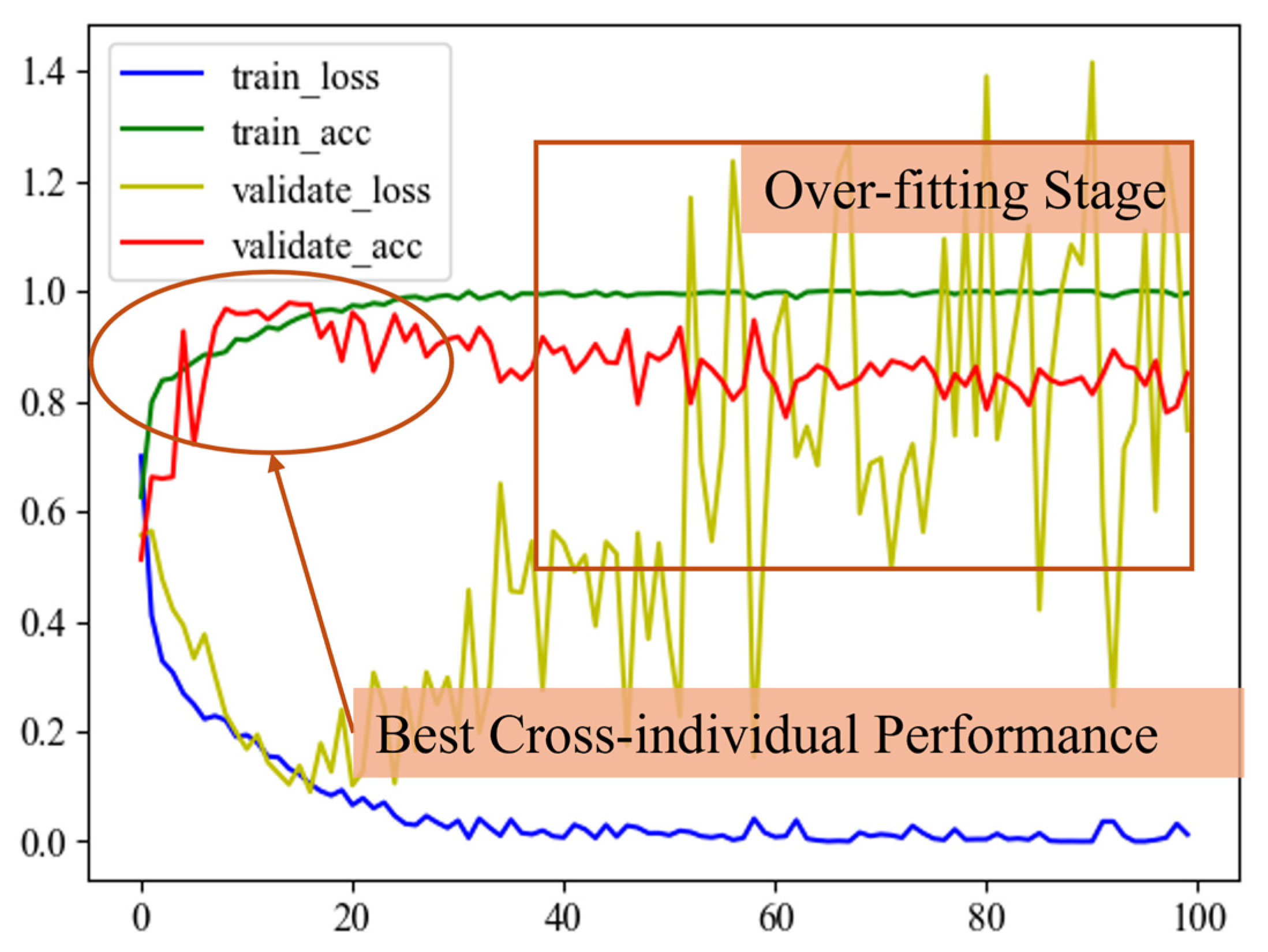
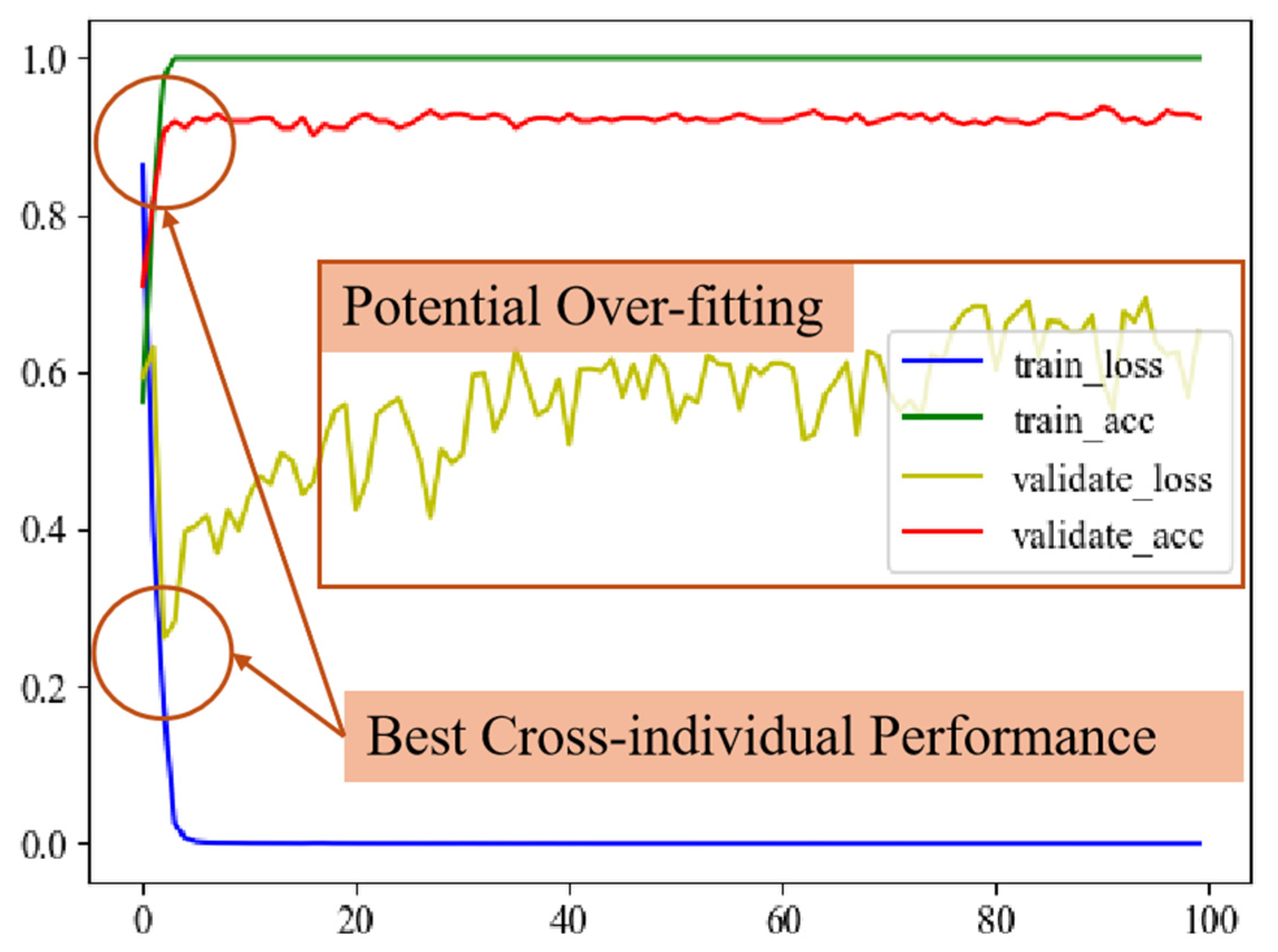
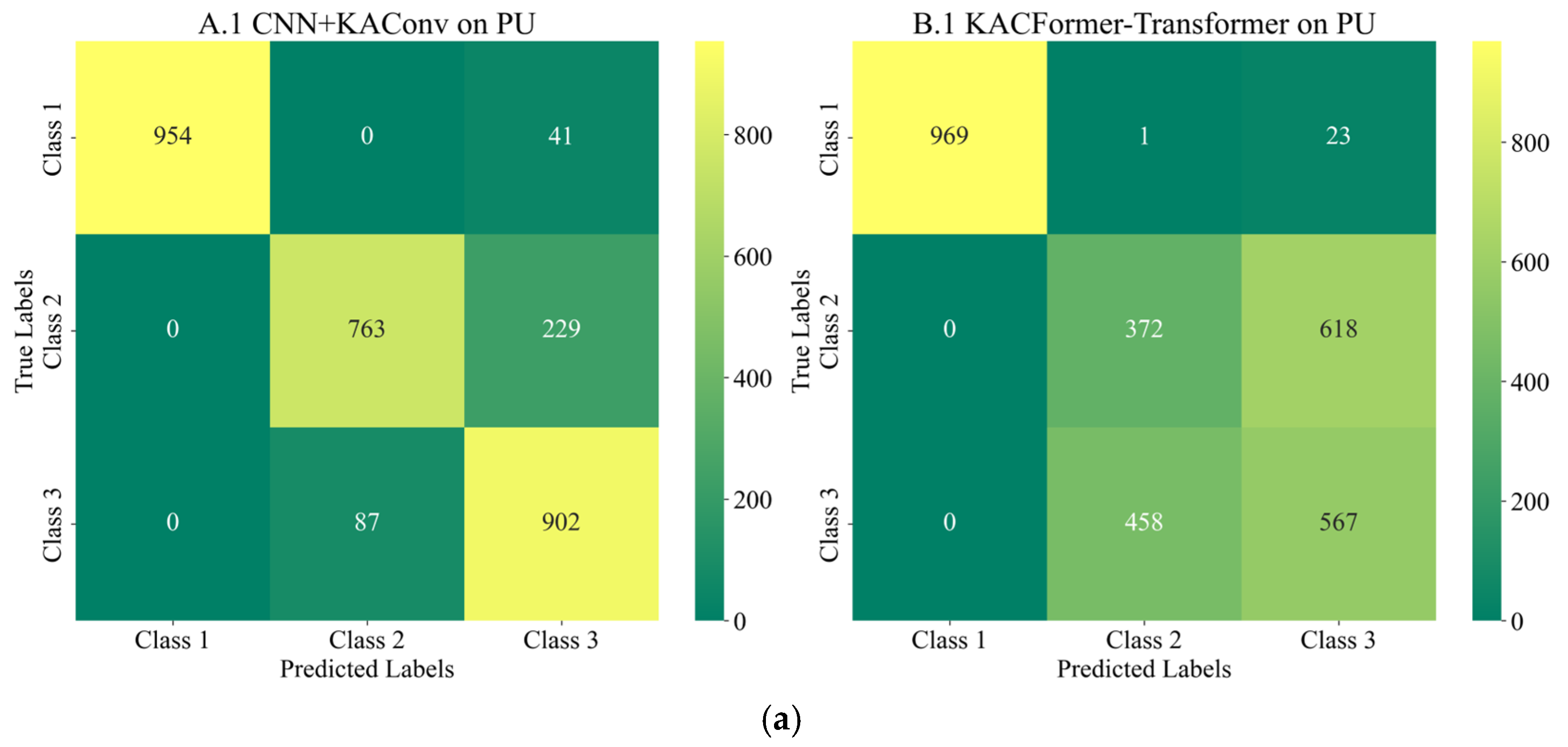
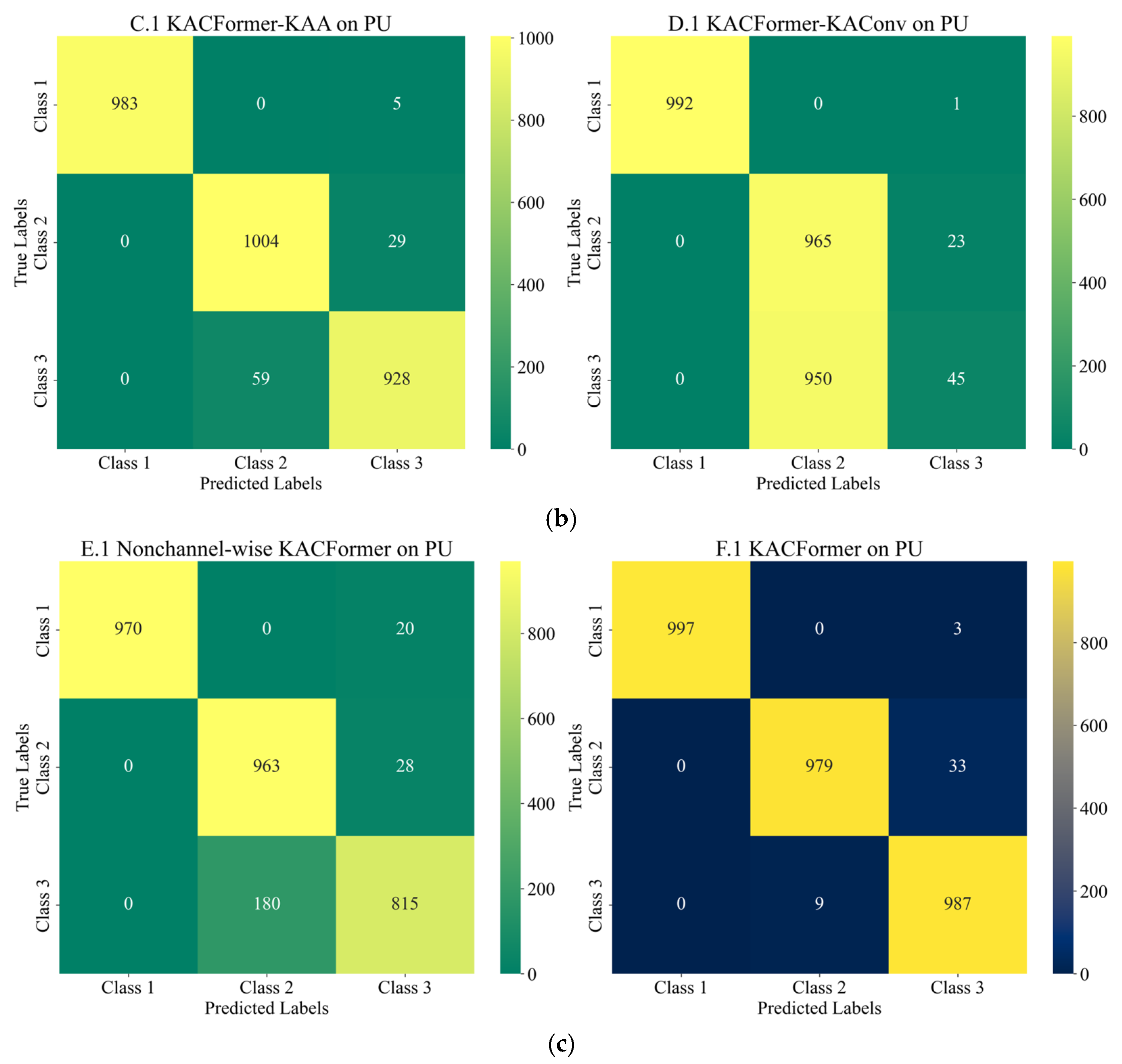
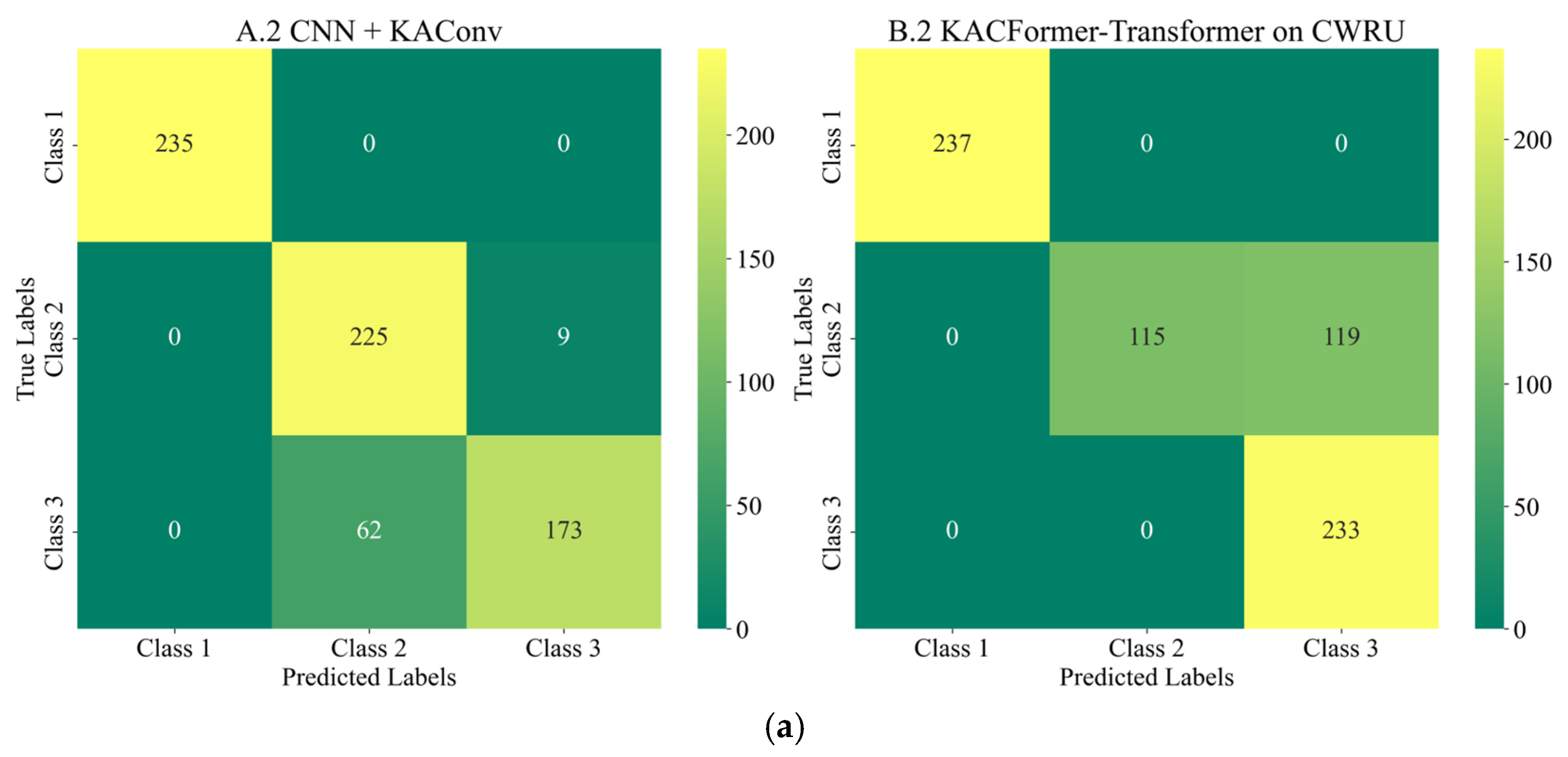
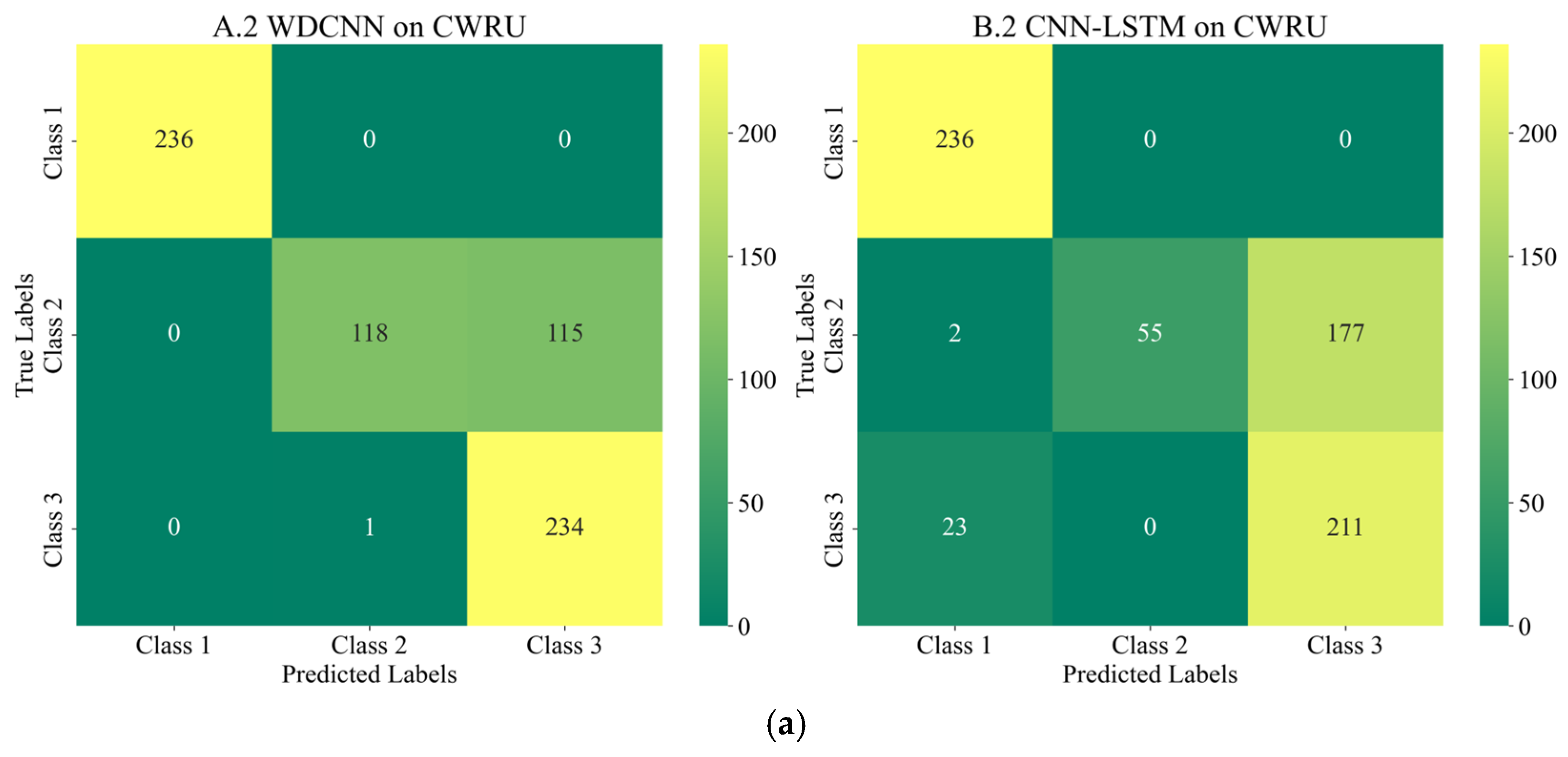
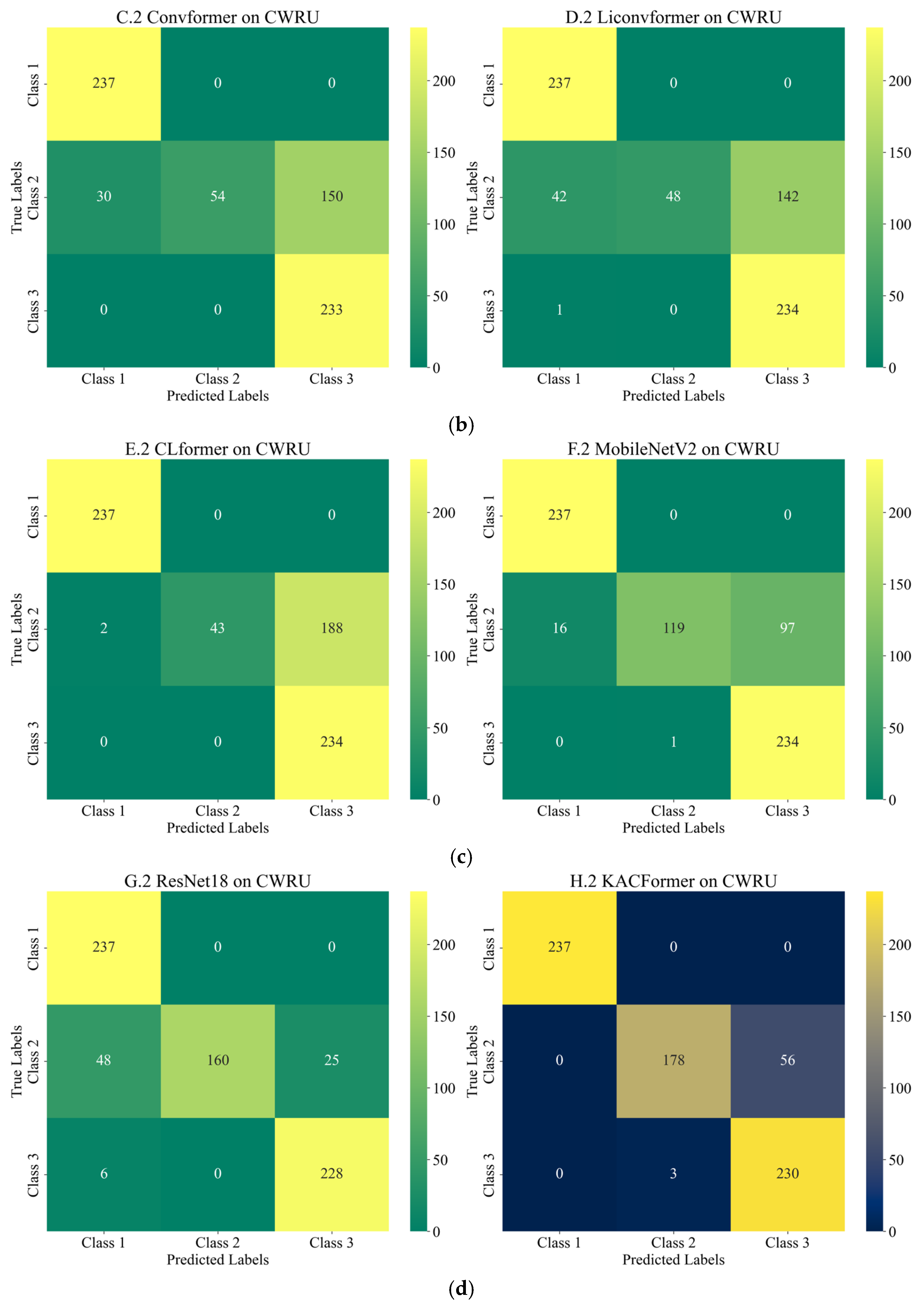
As illustrated in Figure 17, on Task 1, the KACFormer network achieves its best accuracy on the target domain when it begins to converge on the source domain, typically around 5 to 20 epochs. After the 20th epoch, as training continues, the model’s performance on the target domain begins to degrade. Such a phenomenon is not as pronounced on Task 2. As illustrated in Figure 18, the model converges quickly and demonstrates relatively strong stability on the target dataset. However, the rising validation loss may indicate a potential over-fitting risk. Such a difference may be due to the volume of data and the inherent differences between the individuals in target and training datasets. Moreover, as shown in the confusion matrixes listed in Figure 12, Figure 13, Figure 14, Figure 15 and Figure 16, the features of healthy bearings in the PU and CWRU dataset are more distinct compared to the other two categories, and models participating in the experiment demonstrate strong cross-domain performance. However, there is a significant degree of confusion between Inner Race (IR) and Outer Race (OR) faults.

Why SiLU

In the model, the SiLU activation function is employed in the encoder based on experimental validation. This implementation is consistent with the original KAN authors’ use of SiLU activation in their work [16], further validating our design choice. As demonstrated in

Table 8. Model accuracy with different activation functions on different tasks.

	SiLU	ReLU
Task 1 on PU	95.73%	88.74%
Task 2 on CWRU	91.58%	89.98%

, using ReLU activation resulted in accuracy degradation in both tasks compared to SiLU. This performance gap may be attributed to SiLU’s superior properties: smoothness, non-monotonicity, and boundedness below (unbounded above), which make it particularly suitable for approximating smooth functions, and this may be a latent characteristic exhibited in vibration signal processing.

Working Condition

Working condition variability is a widely discussed challenge in fault diagnosis, with numerous scholars dedicated to cross-condition diagnosis [34,35,36]. Since model performance may vary under different operating conditions, considering data availability, experiments are conducted on Task 1 based on the PU dataset—evaluating the same bearing samples under different conditions.

Table 9. Model accuracy under different working conditions.

	N09_M07_F10	N15_M01_F10	N15_M07_F10
Accuracy	95.73%	95.31%	95.36%

presents KACFormer’s accuracy for Task 1 across these three distinct working conditions.

From the experimental data, it can be concluded that when the source domain and target domain individuals work under the same working conditions, the robustness of the algorithm will not be affected.

4. Conclusions

In this work, a cross-individual bearing fault diagnosis scenario is explored. By integrating KART into traditional convolution and attention mechanisms, a novel model, KACFormer, is proposed to explore the potential of leveraging the nonlinear modeling capabilities and individual generalization of KANs. KACFormer enhances feature representation while preserving the translation invariance of convolution and the context-aware semantic modeling ability of attention mechanisms. Extensive experiments on two public datasets demonstrate the superior generalization performance of KACFormer, achieving state-of-the-art accuracy rates of 95.73% and 91.58% in cross-individual scenarios. These results highlight the potential effectiveness of KACFormer in improving fault diagnosis under varying operational conditions and individual differences. Beyond bearing fault diagnosis, the proposed KACFormer framework exhibits potential for generalization to other similar industrial scenarios involving vibration signal processing and domain adaptation, such as health monitoring for gearboxes and wind turbine condition monitoring [37].

Despite the advancement achieved, limitations remain. (1) Compared to MLP-based models, KANs-embedded models take a relatively longer time to train. Further study will be carried out to reduce the complexity of the model while maintaining the cross-individual accuracy. (2) Furthermore, the model should prioritize detecting smaller, incipient faults to better align with industrial requirements, as early-stage fault diagnosis is crucial for predictive maintenance and to minimize machine downtime. However, due to limitations in the current datasets, experiments regarding the model’s minimum detectable fault size were not conducted. This constitutes an important direction for future research.