1. Introduction
Pursuing optimal operational efficiency and safety in complex industrial systems, particularly turbofan engines, hinges on effective predictive maintenance (PdM). While sensor data offers immense potential for anticipating equipment failures, a critical barrier remains: the pervasive scarcity of labeled failure data. This fundamental limitation renders traditional supervised learning approaches largely unfeasible for robust health monitoring and Remaining Useful Life (RUL) prediction in real-world industrial environments [
1].
To address this challenge, this article introduces a novel, entirely unsupervised framework designed for turbofan engines. This comprehensive solution unifies health state classification and RUL prediction, moving beyond fragmented analytical methods. The framework synergistically integrates three advanced machine learning components: autoencoders (AEs) for deep feature extraction, Gaussian Mixture Models (GMMs) for robust unsupervised health state classification (categorizing engines into “Healthy”, “Middle”, and “Unhealthy” states), and state-specific Long Short-Term Memory (LSTM) networks enhanced with Self-Attention Layers (SAL) for accurate RUL prediction.
Rigorous empirical validation on both a large, real-life turbofan engine operational dataset (which crucially lacks explicit run-to-failure labels, mirroring industrial conditions) and the widely used simulated NASA Turbofan Engine Degradation Dataset (CMAPSS) demonstrates the framework’s practical viability and robustness. This unsupervised approach not only effectively captures subtle, high-dimensional degradation patterns but also achieves superior RUL prediction performance compared to numerous state-of-the-art deep neural network models on benchmark datasets, showcasing its competitive advantage.
Recent advances in machine learning for fatigue and life prediction have increasingly emphasized models that can handle data scarcity and uncertainty. For example, Zang et al. [
2] proposed a Gaussian Variational Bayes Network (GVBN) to predict the fatigue life of orthotropic steel bridge deck welds using small-sample experimental data. Their method excels at probabilistic inference under limited data availability and provides posterior distributions over the model parameters, making it highly suitable for structural components with sparse degradation histories. In contrast, our proposed AE-GMM-LSTM-SA framework is designed for multivariate time series data with rich temporal and sensor information, such as those recorded from turbofan engines, and focuses on unsupervised health state discovery and state-specific RUL forecasting. Unlike GVBNs, our method does not assume prior distributions or require Bayesian training; instead, it decomposes the learning process into three interpretable stages: dimensionality reduction via autoencoders, latent clustering with GMMs, and sequential modeling using LSTM with self-attention. Furthermore, our approach is designed to scale to large unlabeled industrial datasets and supports early RUL forecasting, a requirement critical for proactive maintenance in aviation. While GVBNs are well-suited for small, structured fatigue datasets, the proposed framework addresses a complementary class of problems involving high-dimensional, nonlinear degradation dynamics under weak supervision.
The remainder of this article provides a detailed exploration of the presented framework, its methodology, empirical results, and a comprehensive discussion of its industrial applicability, limitations, and future directions.
2. Literature Review
2.1. Background and Motivation for Predictive Maintenance
Predictive maintenance (PdM) [
3,
4] has emerged as a critical strategy in modern industries for reducing unplanned equipment downtime, extending asset lifespans, and optimizing operational costs [
5]. Unlike reactive or scheduled maintenance, PdM aims to anticipate failures by analyzing real-time operational data [
6] to determine the health status of equipment and forecast Remaining Useful Life (RUL) [
7,
8]. This approach is particularly vital in high-stakes sectors such as aviation, in which component failure can have severe safety and financial implications.
In the aviation industry, jet engines are subject to varying environmental and operational conditions that lead to complex degradation behaviors. Traditional maintenance strategies often fall short due to their reliance on rigid schedules or post-failure interventions. Consequently, there is a growing demand for intelligent systems capable of monitoring engine health and predicting failures in advance.
2.2. Limitations of Traditional and Supervised Approaches
Historically, predictive models have relied on physics-based simulations and supervised machine learning. While physics-based models benefit from domain knowledge [
9,
10,
11], they often require explicit failure definitions, are time-consuming to develop, and may not generalize well to new failure modes [
12,
13]. On the other hand, supervised machine learning approaches require extensive labeled datasets, often unavailable in industrial settings due to the difficulty of accurately labeling large volumes of sensor data or the scarcity of failure events.
This scarcity introduces a bottleneck in supervised learning applications and limits the scalability of PdM systems. The labeling process is labor-intensive and prone to inconsistencies, especially in cases where failure progression is gradual or ambiguous. Furthermore, real-world operational data rarely includes run-to-failure records, complicating the application of supervised learning frameworks [
14].
2.3. The Shift Toward Unsupervised Learning
In response to these limitations, the research community has increasingly turned to unsupervised learning methods, which identify patterns and anomalies in unlabeled data [
15,
16,
17,
18,
19]. These techniques are especially useful for applications in PdM, where equipment failures are rare and labeling is impractical. Unsupervised methods are particularly advantageous in scenarios where failure modes are poorly understood or evolve, as they enable adaptive modeling of equipment degradation [
20,
21].
Among the most prominent unsupervised methods are autoencoders and Gaussian Mixture Models (GMMs) [
22,
23]. Autoencoders, a type of neural network, are used for compressing high-dimensional sensor data into lower-dimensional latent spaces that capture essential features [
24,
25,
26]. Variants such as variational and denoising autoencoders further improve performance in noisy or incomplete datasets [
27,
28,
29].
Among unsupervised techniques, dimensionality reduction and clustering algorithms have gained prominence for their ability to distill high-dimensional sensor data into actionable insights. Principal Component Analysis (PCA) and t-SNE are widely employed to visualize and interpret multivariate sensor streams [
30,
31], while clustering methods like K-means partition data into distinct health states [
23]. Clustering methods, such as GMMs and K-means, categorize equipment states (e.g., healthy, degraded, faulty) without prior labels. GMMs are particularly suited for industrial sensor data due to their probabilistic foundation, which handles overlapping clusters and non-uniform distributions better than hard clustering methods like K-means [
32,
33,
34,
35].
2.4. Existing Approaches in Unsupervised PdM
Several studies have successfully demonstrated the use of unsupervised learning for equipment monitoring. For instance, Li et al. [
17] validated the robustness of autoencoder-based models in detecting early-stage anomalies under limited labeled data [
34,
35]. Sayah et al. [
22] introduced a hybrid framework combining LSTM networks with GMM clustering, showing improved accuracy in RUL prediction.
Recent work has explored neuro-fuzzy and observer-based approaches for unsupervised fault diagnosis in wind turbines. For instance, Pérez-Pérez et al. (2024) introduce a robust diagnosis method that uses a Multiple-Output ANFIS (MANFIS) to derive Takagi–Sugeno models, coupled with a bank of zonotopic state estimators for residual generation [
36]. In a related study, Pérez-Pérez et al. (2023) present a hybrid FDI approach in which an ANFIS identifies quasi-Linear Parameter Varying (qLPV) models of the turbine, and a bank of qLPV zonotopic observers then detects sensor and actuator faults—notably, this method is trained only on fault-free data [
37]. Another recent work (Pérez-Pérez et al., 2022) employs an ANFIS to obtain a convex Takagi–Sugeno interval model of the turbine and designs convex state observers; fault diagnosis is performed by generating residuals from these observers, again using only healthy data for training [
38]. These studies demonstrate that advanced neuro-fuzzy identification and interval/zontopic observer methods can effectively classify or isolate unlabeled faults in wind turbine systems.
Hybrid models that combine unsupervised and supervised components, such as Autoencoder-GMM for classification followed by LSTM for RUL estimation, have shown promising results in capturing both spatial and temporal degradation patterns [
39,
40,
41,
42,
43,
44]. Attention mechanisms further enhance these models by prioritizing critical features in time-series data [
8,
45,
46,
47].
To summarize, it is worth emphasizing that all the literature mentioned and the elaborations presented by Waters et al. (2022) [
48], Saucedo-Dorantes et al. (2021) [
49], and Komorska and Puchalski (2024) [
50] underscore the growing trend of applying deep learning and unsupervised techniques in predictive maintenance, particularly in scenarios with limited labeled data.
3. Motivation and Research Problem
In many real-world applications, such as predictive maintenance, it is crucial to classify equipment’s health state and predict its Remaining Useful Life (RUL). However, obtaining labeled data for training supervised models is often challenging due to the excessive cost and effort involved in manual labeling. This creates a significant gap in effective monitoring and maintenance of equipment.
While several unsupervised learning techniques have been proposed for similar problems, comprehensive methodologies that combine autoencoders and GMMs for classification and RUL prediction are lacking. GMMs assume that data points are generated from a mixture of Gaussian distributions. Unlike K-means, GMMs accommodate clusters of varying shapes and sizes, making them suitable for complex industrial data. K-means and hierarchical clustering struggle with overlapping clusters and high-dimensional data. GMMs’ probabilistic framework addresses these issues by modeling covariance structures.
Among the most common recent techniques applied for equipment RUL estimation and prediction are the following:
LSTM networks to capture temporal dependencies in sensor data [
51,
52].
Hybrid models to combine CNNs for spatial features and LSTMs for temporal dynamics.
Physics-based models use domain knowledge but require explicit definitions of failure modes.
Despite these advancements, several challenges remain:
Unified frameworks: Most existing work treats health state classification and RUL prediction as separate tasks. A unified model that integrates both functions within an unsupervised framework is rare.
Data limitations: Real-world datasets lack run-to-failure labels, making supervised training infeasible. Existing studies often rely on simulated datasets like CMAPSS, which do not reflect the complexity of actual operations.
Interpretability: Industrial adoption requires that clustering results and RUL predictions be explainable to engineers and decision-makers [
53,
54].
These gaps highlight the need for an end-to-end unsupervised solution that bridges classification and prognostics without labeled data.
This article addresses these limitations by proposing a hybrid framework that synergizes autoencoders for feature compression, GMM for unsupervised health-state classification, and LSTMs for state-specific RUL prediction, implemented and validated on both real-life and simulated turbofan engine data. By unifying these components, the methodology eliminates reliance on labeled training data, offering a scalable solution for industrial applications where failure histories are incomplete or unavailable.
The methodology is implemented in MATLAB, and the results are analyzed to demonstrate its effectiveness. The specific objectives are as follows:
Develop a hybrid model integrating autoencoders for feature extraction and GMMs for clustering.
Provide a mathematical and algorithmic foundation for each component.
Implement and validate the framework using MATLAB R2024b on the NASA CMAPSS Turbofan Engine Degradation Dataset, as well as the real-life engine operational data.
Compare performance against supervised benchmarks.
4. Methodology
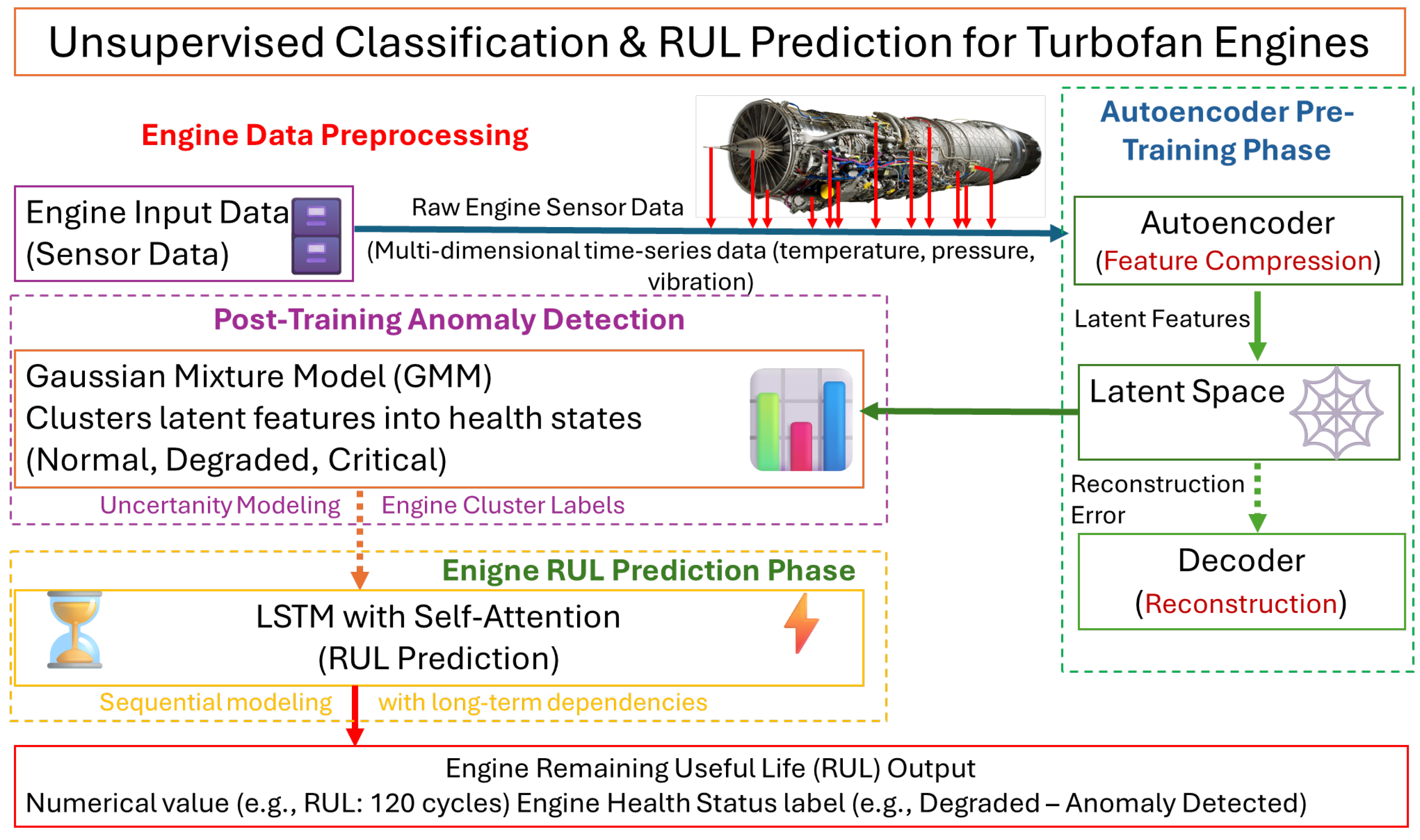
The proposed methodology consists of the following steps:
Data Preprocessing to normalize and prepare the data for analysis.
Feature Compression Using Autoencoder to train an autoencoder to learn a compressed representation of the input data.
Unsupervised Classification Using GMM: GMM application to classify the compressed features into distinct engine states.
RUL Prediction: Training separate LSTM models for each engine state to predict RUL.
Evaluation: Engine classification performance evaluation and RUL prediction using RMSE, R-squared, and Score metrics.
Figure 1 presents a designed neural network model for the unsupervised classification using autoencoders and Gaussian mixture models for turbofan engine RUL prediction.
4.1. Data Preprocessing
The first step in the methodology is to preprocess engine data. The dataset, stored in a MATLAB file, includes engine SNs, cycle counts, and sensor measurements. Features are extracted from columns and organized into cell arrays where each cell corresponds to a specific engine. Data preprocessing involves normalizing features to ensure uniformity and that they are on a similar scale. The dataset used in this study contains sensor readings and operational parameters for multiple engines. Each engine has a varying number of cycles, and the goal is to classify the engines into health states (Healthy, Middle, Unhealthy) and predict their RUL.
4.1.1. Dataset Description
Two engine datasets were used in the current case study:
Real-life Engine Operational Data: This primary dataset was collected from a fleet of modern, powerful low-bypass turbofan engines over 12 years of flight and ground operations. It comprises 43,472 records collected for 53 individual engines. Data was gathered from 12 engine sensors and 2 aircraft signals. While there are 12 physical sensors, 86 different parameters are recorded as “Performance Data”. The dataset includes columns, representing various parameters like ESN (Engine Serial Number), Time, Total temperature at station 2 (TT2), Mach number, Power Lever Angle (PLA), sensor readings (e.g., Pt2, PbC), operational conditions, and derived metrics (e.g., Total Accumulated Cycles TACS, Engine Operating Time EOT2). Each row represents a snapshot of data for a specific engine on a given flight. The Engine Monitoring System (EMS) records one set of averaged engine operating parameters during every aircraft takeoff. This specific flight phase is crucial, as it demands maximum thrust, subjecting the engine to its greatest stresses and loads, which significantly impact its condition and health status. This makes takeoff data highly reflective of engine performance, efficiency, and degradation. Though 86 parameters were recorded, only degradation-sensitive features are retained through autoencoder compression. Core sensors like TT2 (compressor health), Pt2/PbC (airflow integrity), and derived metrics TACS/EOT2 (cumulative wear) are critical for failure prediction. Mach number and PLA provide operational context for stress normalization. Crucially, this real-life dataset is not run-to-failure data, meaning that the exact engine status, failure moment, and Remaining Useful Life (RUL) for each engine are unknown. This scenario is very common in real-world operational datasets collected over many years. The whole real-life engine operational data originates from the fleet of F100-PW-229 Pratt & Whitney turbofan engines.
NASA Turbofan Engine Degradation Dataset (CMAPSS): This is a widely used simulated dataset, employed in this study to prove the effectiveness of the designed model and enable comparison with other models existing in scientific publications. Unlike the real-life data, CMAPSS data is run-to-failure data, in which engines reach their failure moment in the last recorded set of parameters. The CMAPSS dataset consists of four sub-datasets (FD001, FD002, FD003, FD004), and the results presented in this paper for CMAPSS are often the mean performance across these sub-datasets.
Both datasets contain sensor data (e.g., temperatures, pressures sensed at various engine cross-sections, RPM, airflow, fuel metered) from the engines, as well as environmental data and thermodynamic parameters calculated during engine operation.
4.1.2. Normalization and Feature Engineering
The following step of the presented methodology is data normalization. This step is, in the case of deep neural networks, extremely important. Engine data consists of data that might be of diverse types and ranges. Examples of data with diverse types and precision are single, double, integer, integer8, long, etc. For neural network data processing, it is important to normalize the data. Otherwise, the design model could fail to converge or result in poor network accuracy. In this case study, the standardized dataset has a mean of 0 and a standard deviation of 1, which allows data symmetry and distribution.
4.2. Autoencoder Implementation
Autoencoder network architecture was selected for engine feature learning. Autoencoders (AEs) are neural networks trained to reconstruct inputs through a bottleneck layer, forcing the model to learn compressed representations. Variants include the following:
Denoising Autoencoders: Robust to noisy inputs.
Variational Autoencoders (VAEs): Probabilistic latent space modeling.
Sparse Autoencoders: Enforce sparsity constraints for interpretability.
AEs have proven to have successful applications in predictive maintenance. They have been used to detect bearing, gear, and turbine anomalies by reconstructing healthy operational data and flagging deviations.
4.2.1. Feature Compression Using Autoencoder
Before engine state classification, engine datasets must be processed through the encoder–decoder-type neural network. Such a network architecture allows the conversion of various engine data sequences [
55] into the compressed dataset, which is then converted into the vectors of engine parameters, which might be easily processed into engine state clusters. An autoencoder is a neural network that learns a compressed input data representation. It consists of an encoder that compresses the input data into a lower-dimensional representation and a decoder that reconstructs the input data from the compressed representation.
4.2.2. Autoencoder Architecture
How is the engine dataset processed through the encoder? Let us assume that the input engine data is represented as
. The encoder maps
to a latent representation of
, where
in accordance with Equation (1):
where
and
are the weights and biases, while
is a nonlinear activation; in this scenario, it is a ReLU activation layer.
4.2.3. Decoder Function
The decoder reconstructs the engine input data from
in accordance with Equation (2).
How was the autoencoder architecture designed? At the entrance of the autoencoder layer was the sequence input layer with the size of the engine input data. The encoder consists of two fully connected layers (128 units) with ReLU activation. The following layer was the bottleneck layer: the 32-unit layer. The decoder layer was designed symmetrically to the encoder. Following the decoder was the output layer, which was the fully connected layer matched to the size of the data. The last layer was the regression layer.
To train the autoencoder neural network, various training options were tested to achieve the best results. Hyperparameters (layer sizes, dropout rate, epochs) were selected via grid search and performance analysis. For the autoencoder, we evaluated bottleneck dimensions {16, 32, 64}, dropout rates {0.1, 0.2, 0.3}, and epochs {200, 300, 400} on a validation set (10% of training data). The configuration minimizing reconstruction loss (RMSE) and RUL prediction error was adopted: a 32-unit bottleneck, a dropout of 0.2, and 400 epochs. As a training optimizer, Adam was selected with a learning rate of . To prevent overfitting, regularization with a 0.2 dropout rate was set. The mini-batch sequence size was set at 8.
4.3. Unsupervised Classification Using Gaussian Mixture Model (GMM) Clustering
A GMM is a probabilistic model that assumes the data is generated from a mixture of Gaussian distributions. It is used to classify the compressed features into distinct engine states.
The GMM models engine data as a weighted sum of K Gaussian distributions. The probability density function can be calculated in accordance with Equation (3).
where
are mixing coefficients
, and
denotes a Gaussian with mean
and covariance
.
Feature Aggregation
Having trained the autoencoder model, compressed features were extracted for each engine. Then, the engine features were aggregated per engine and standardized.
GMM clustering was performed to classify engines into three states: Healthy, Middle, and Unhealthy. Cluster indices were mapped to engine states, and clustering results were visualized by plotting aggregated and compressed features vs. their values. Health states emerge from GMM clustering of compressed features, not predefined thresholds. Lower latent values (Healthy) correspond to nominal sensor baselines, while higher values (Unhealthy) reflect deviation magnitudes. For example: 20% Δ in exhaust gas temperature → Middle state; 35% Δ in vibration amplitude → Unhealthy state. This progression aligns with physical degradation models in which early faults manifest as subtle deviations before accelerating toward failure.
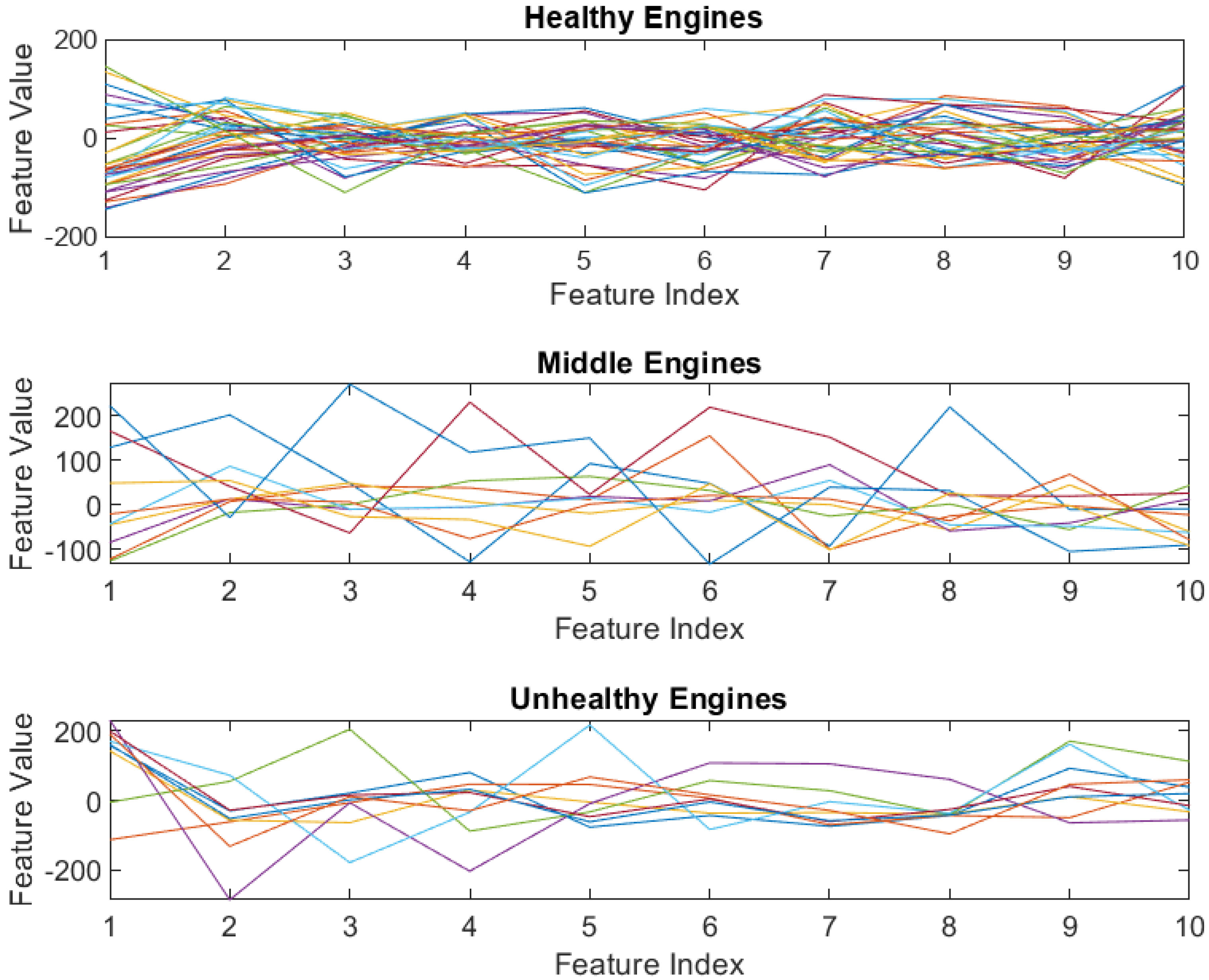
Visualized results for one of the results are presented in
Figure 2.
Figure 2 illustrates the distribution of compressed engine features classified by the GMM into three distinct health states: Healthy, Middle, and Unhealthy. Every colored line refers to the individual engine serial number. As observed, the range of values for crucial compressed engine features tends to be lower for Healthy engines, progressively increasing for Middle engines, and significantly higher for Unhealthy engines. While feature values provide an indication, the trend of these values over time truly signifies changes in engine health status. For the real-life engine dataset, distinguishing clear trends for the Middle and Unhealthy engines presents a significant challenge, highlighting the inherent complexity and noise in real-world operational data.
4.4. LSTM-Based RUL Prediction with Self-Attention
4.4.1. RUL Prediction Model Architecture
How was engine RUL predicted? Once the engines are classified into distinct states (Healthy, Middle, and Unhealthy), separate LSTM models are trained for each state to predict RULs. A RUL prediction model designed whose architecture was based on the following layers: the Sequence Input Layer, with the size of the engine data clustered to one of the engine health states; the LSTM Layer, with 128 units with sequence output; followed by the Dropout Layer. The LSTM unit count (128) aligned with similar architectures in [
39,
41]. One of the essential layers was the Self-Attention Layer (SAL), with eight heads and eight key dimensions. SAL was connected to the fully connected layer with 32 hidden units and ReLU activation layer, again followed by a fully connected layer and a regression head being fully connected layer with linear activation. Again, some neural network training options were based on the model performance metrics, starting from 100 epochs and 32 mini-batch sizes through 200 and 16, finishing with 400 epochs and a mini-batch size of 8. The initial learning rate was set at 0.001. Before neural network training, each engine state was divided into two subsets: training and testing, with a 0.8-to-0.2 division ratio. Beyond the 80/20 split, 5-fold cross-validation was performed per health state to ensure robustness. Mean RMSE variations were <5% across folds, confirming stability. For the GMM, cluster consistency was verified via repeated initialization (10 runs), yielding <3% label assignment variance.
4.4.2. Loss Function and Metrics
While training the LSTM-based RUL prediction model, the neural network tries to minimize the loss function. The RUL prediction network is trained as a regression model using the Mean Squared Error (MSE) loss between predicted and actual remaining life.
The most popular and common performance metrics were applied to evaluate neural network performance. Many various metrics are used in NN applications, but there is no one standard set. That is why it was decided to use the Root Mean Squared Error RMSE, Coefficient of Determination R2, and Score function for comparison with other RUL prediction models from the literature.
5. Results and Analysis
5.1. Autoencoder Performance
Reconstruction Error
To evaluate autoencoder performance, reconstruction error, measured as the RMSE between the real engine data set and the reconstructed data set, was calculated.
Reconstruction error of 5.20 × 10⁻² was achieved, while the loss function converged to 6.3 × 10⁻². These values indicate that the autoencoder can reconstruct the high dimensional sensor inputs with an average RMSE of 0.052, and that the training loss (0.063) converged to a similar level. The small difference between reconstruction error and loss demonstrates stable training with minimal overfitting, confirming that the latent representation retains the essential structure of the original data.
5.2. GMM Clustering Results
5.2.1. Cluster Separation
The GMM application for the engine dataset classified each engine into one of the clusters. Every cluster corresponds to one of the engine health states: Healthy, Middle, or Unhealthy. Eventually, 57% of engines fell into the first class, 36% into the middle, and 7% into the third.
The silhouette performance metric was used to validate GMM clustering performance. It quantifies how well each data point fits into its assigned cluster compared to other clusters, balancing two key concepts: cohesion and separation. The first one defines how close a data point is to other points in its own cluster. The second one explains how distinct a data point is from points in other clusters.
For the real-life engine operational dataset and GMM clustering, the achieved silhouette performance was equal to 0.12. This silhouette score (0.12) implies weak but meaningful separation. In real world engine signals characterized by measurement noise and gradual degradation, such modest separation is expected. This low value stems from gradual degradation transitions in real engines, unlike sharp failure boundaries in simulated data (silhouette = 0.39).
One of the most significant differences between GMM and K-means clustering is that the latter is a hard clustering method. It means that it works by associating each point with one and only one cluster. There is no uncertainty or probability measure of how much each data point is associated with a specific cluster.
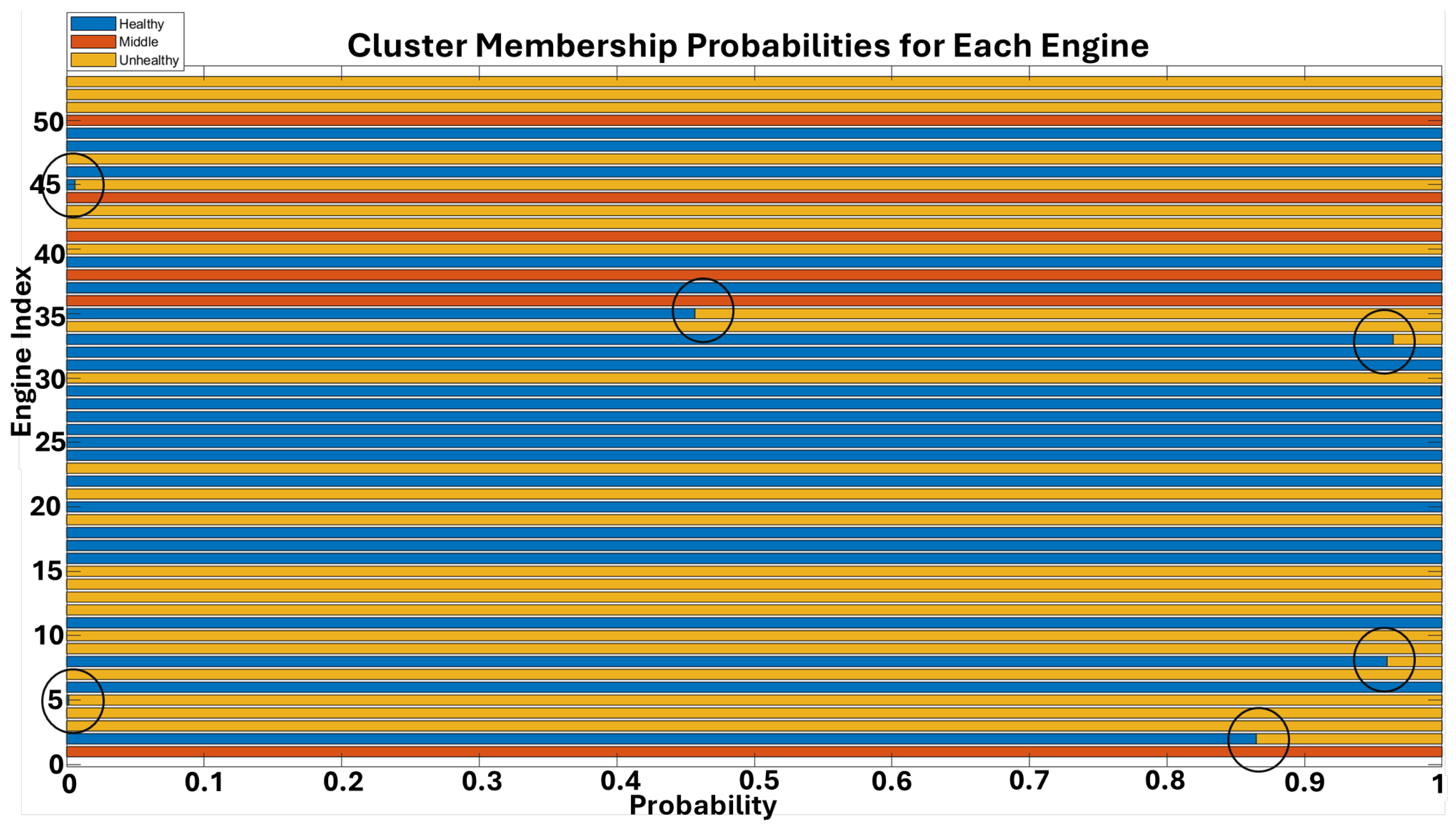
That was the reason why it was decided to calculate the average clustering probability and posterior probabilities for each engine. The first metric shows how confident the model is in its cluster assignments on average, and the achieved result was 0.99. The posterior probabilities for each engine were calculated and are presented in
Figure 3. As a result of posterior calculations, a matrix was returned where each row corresponds to an engine, and each column gives the probability of belonging to the respective cluster (Healthy, Middle, Unhealthy). Unfortunately, only for a few engines, clustering confidence is easy to recognize in the diagram. Still, for all the engines, cluster membership probability never reaches 1. There are always some residual probabilities for other engine health states.
Figure 3 displays the GMM cluster posterior probability distributions for individual engines across the three identified health states. Each row represents an engine, and the color intensity indicates the probability of that engine belonging to a specific cluster (Healthy, Middle, or Unhealthy). While the average clustering probability was high (0.99), suggesting overall confidence in assignments, the figure reveals that for most engines, cluster membership probability does not reach 1. This indicates that there are often residual probabilities for other health states, reflecting the inherent ambiguity and gradual transitions between degradation stages in real-world engine data. Only for a few engines is the clustering confidence distinctly clear in the diagram.
5.2.2. Comparative Analysis
Since the proposed model was one of the few in the literature trained and tested on real-life engine operational data, it was difficult to compare the results to other proposed models. To overcome this issue, it was decided to apply the proposed model to the most used literature engine data, the CMAPPS data.
The reconstruction error for the CMAPPS engine dataset was equal to 1.34 × 10⁻², while the loss function converged to 2.6 × 10⁻³.
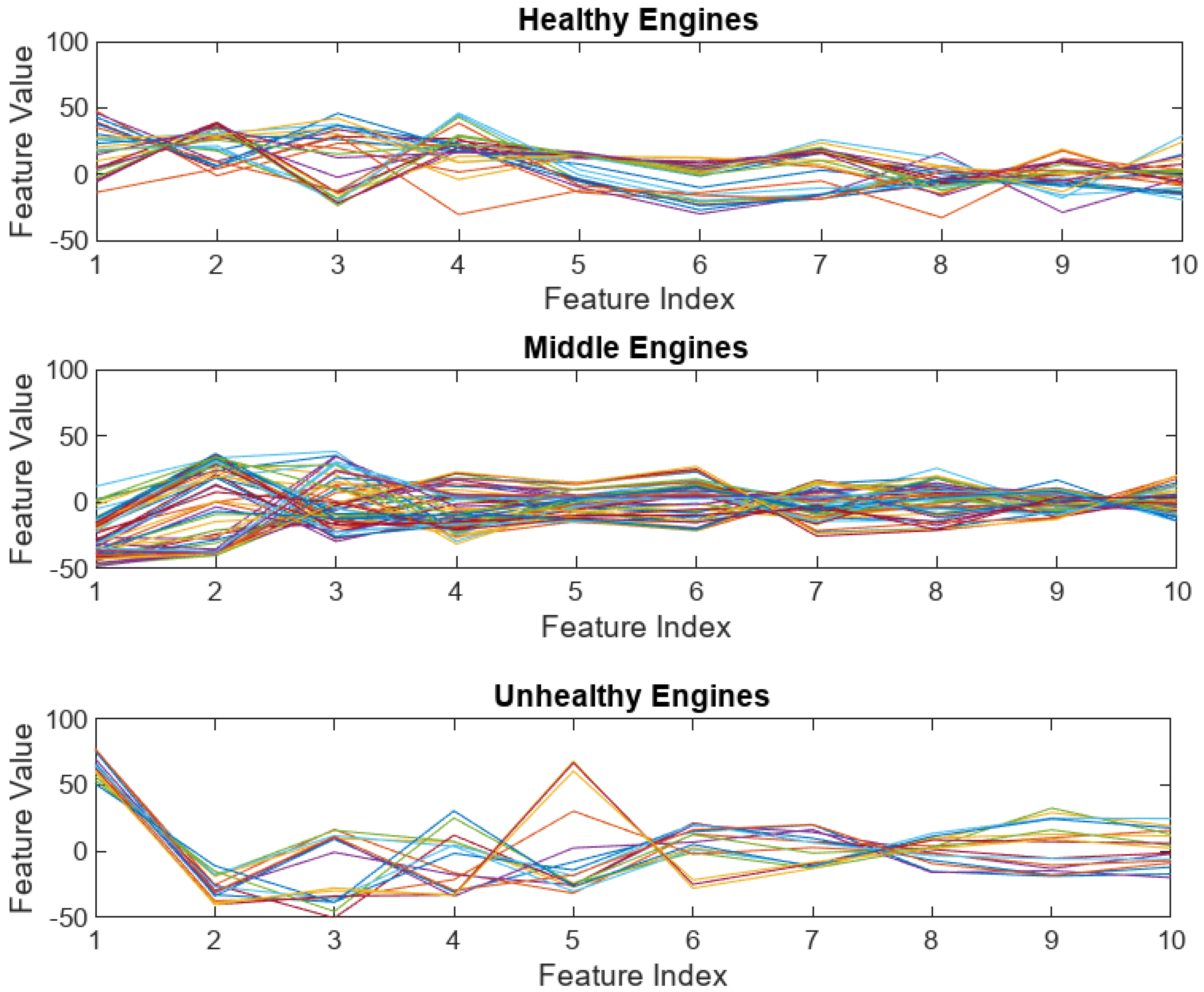
In
Figure 4, GMM clustering results for the CMAPPS dataset are presented.
Figure 4 presents the GMM clustering results for the CMAPSS dataset. In contrast to the real-life data, the CMAPSS data shows clearer distinctions in engine feature trends, particularly for Unhealthy engines. The feature values for Unhealthy engines exhibit a notably wider range (from −53 to +77) compared to the other two health states, making their trendability quite evident. This observation supports the conclusion that simulated engine datasets are generally easier to model and simulate than real-life engine datasets, which are collected over many years under diverse environmental conditions and contain more inherent noise and variability.
To improve the visualization of the GMM clustering, the PCA analysis was applied to the CMAPPS and real-life engine data. The results were presented in
Figure 5 for the CMAPPS data (a) and real-life engine data (b). PC1 (68% variance) captures overall degradation magnitude; PC2 (12% variance) isolates fault modes. Healthy engines cluster tightly (bottom-left), while Unhealthy engines disperse along PC1 (right) due to varied failure signatures. Middle states bridge this continuum.
Figure 5 illustrates the GMM engine health state clustering results projected onto a 2D space using Principal Component Analysis (PCA). In this projection, each sample corresponds to an aggregated latent feature vector extracted by the autoencoder, representing an engine’s overall health state averaged over time.
Figure 5a displays the clustering for the CMAPSS engine dataset, which consists of 20,631 engine records from 100 engine serial numbers. For CMAPSS, 58 samples were assigned to the Healthy condition, 31 to Middle, and 11 to Unhealthy.
Figure 5b shows the clustering for the real-life engine operational data, comprising 43,472 records from 53 separate engines. For the real-life data, 9 engines were classified as Healthy, 34 as Middle, and 10 as Unhealthy. The silhouette performance for CMAPSS GMM clustering was 0.39, which is approximately 70% better than the 0.12 achieved for the real-life engine operational dataset. This significant difference in silhouette scores visually confirms that the simulated data is considerably easier to model and process due to its clearer separation of health states compared to the more complex and noisy real-life data.
For the CMAPPS engine dataset and GMM clustering, the achieved silhouette performance was equal to 0.39. This result is about 70% better for the simulated data. This result confirms the assumption that the simulated data is much easier to model and process than the real-life one.
5.3. RUL Prediction Accuracy
In
Table 1, a comparison of the RUL prediction accuracy calculated for the proposed neural network performance metrics and the two described datasets is presented.
Root Mean Square Error (RMSE) is a common neural network performance metric. The RMSE for the CMAPPS engine dataset ranged from 5.057 for the Unhealthy engine state to 12.947 for the Middle engine state. This was up to an order of magnitude lower than the RMSE achieved for the real-life engine operational dataset, which ranged from 62.618 for the Healthy engines to 130.201 for the Unhealthy engines. Comparing the R-squared performance metric of the two datasets, it may be concluded that the difference was not remarkably high and ranged from 2.1 to 12.8%. For the CMAPPS data, the achieved R-squared was close to 1, reaching 0.986 for the Unhealthy engine condition. Such a situation confirms the quality of the proposed model, which defines how well the engine model reflects real engine RUL.
One of the crucial neural network performance metrics assessing engine RUL prediction is the Score function. This metric penalizes so-called late predictions, which means that the predicted engine RUL is higher than the real engine RUL. For the CMAPPS engine data, the achieved Score was close to zero. Unfortunately, the Score function was negative, which means that the predicted RUL is greater than the real one. However, looking at the real values, it was found that the difference is within the assumed tolerance range. In this case, it was five cycles, which is about 0.45% (on average) of the real engine’s remaining useful life.
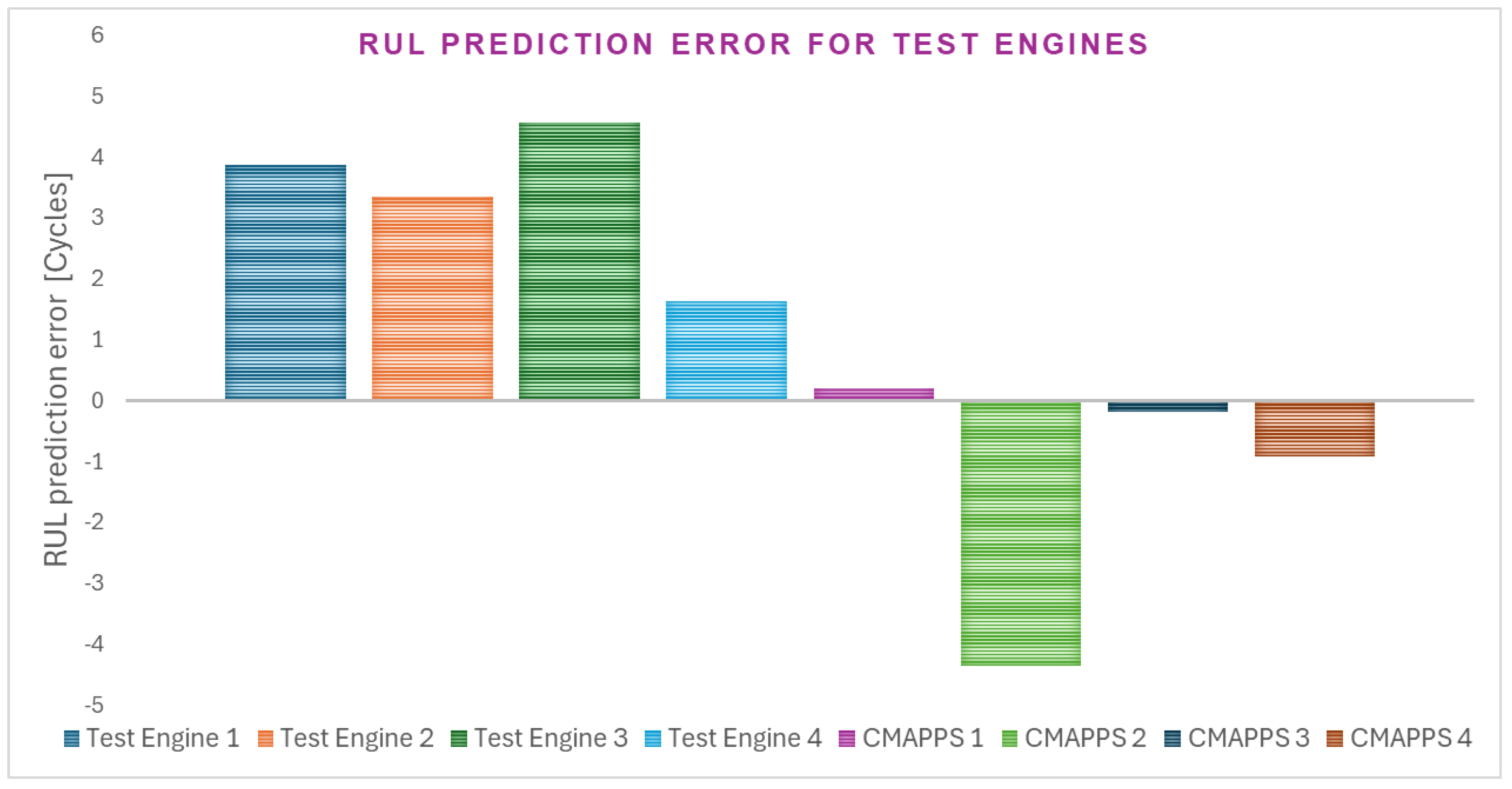
Figure 6 presents the selected test engines’ CMAPPS and real-life RUL prediction errors.
Figure 6 illustrates the RUL prediction error for selected test engines from both the CMAPSS and real-life engine datasets. The figure provides a visual representation of the deviation between the predicted RUL and the actual RUL for individual engines. RUL prediction error is a crucial performance metric. Its significance lies in its specific consideration of situations where the predicted RUL value is lower than the real value. This is paramount for aviation safety, as a late RUL prediction (i.e., predicting a higher RUL than the actual remaining life) could lead to an in-flight engine failure, potentially resulting in an aircraft incident or accident. The RUL for all selected real-life test engines was positive, which indicates an early prediction (the model predicts failure before it happens). For 3 out of four selected CMAPPS test engines, the RUL prediction error is negative, which indicates a late or on-time prediction (the model predicts failure at or after it happens).
Regarding the loss value (
Table 1), results achieved for the CMAPPS dataset ranged from 0.079 for the Middle-state engines to 0.207 for Unhealthy engines. What was surprising was that despite the real-life engine dataset being full of noisy signals and plenty of outliers resulting from sensors’ nuisance readings, the final loss results were lower, to the order of magnitude for Healthy and Unhealthy engines, with comparable results for the Middle ones. This suggests that while the real-life data is more challenging, the model’s training process was able to converge effectively, indicating its robustness.
6. Discussion
6.1. Industrial Applicability
The proposed framework combining autoencoders and Gaussian Mixture Models (GMMs) for unsupervised classification and Remaining Useful Life (RUL) prediction demonstrates significant industrial applicability. By eliminating the need for labeled data, the method enables scalable implementation across various industrial sectors, including aviation, manufacturing, and power generation. Predictive maintenance strategies based on this approach can lead to a substantial reduction in unplanned downtime and maintenance costs. The ability to classify engine health states without supervision provides a reliable early warning system for potential failures, allowing for proactive maintenance scheduling.
One of the major benefits of the methodology is its adaptability to real-world engine datasets. Unlike the NASA CMAPPS dataset, real-life engine operational data does not contain explicit failure labels, making supervised learning techniques difficult to apply. By leveraging unsupervised learning, the proposed framework successfully addresses this challenge, making it a practical solution for industries in which failure data is limited or unavailable.
6.2. Methodological Insights
The combination of an autoencoder and a GMM provided a robust feature extraction and clustering mechanism. The autoencoder efficiently compressed high-dimensional sensor data into meaningful latent representations, preserving essential information while reducing computational complexity. The GMM then effectively categorized engines into distinct health states based on the extracted features.
A key finding from the study is the ability of the GMM to capture the natural structure of the data without predefined labels. This probabilistic clustering method, in contrast to K-means, successfully handles overlapping clusters and varying distributions of engine states. Furthermore, the evaluation metrics, particularly reconstruction error and cluster separation results, indicate that the model performs well in differentiating between healthy, middle, and unhealthy engine states.
The application of LSTM networks for RUL prediction demonstrated promising results, particularly in capturing temporal dependencies in sensor data. By training separate LSTM models for each health state, the framework enhanced prediction accuracy. The integration of self-attention layers further improved the model’s ability to focus on critical temporal patterns, enhancing its predictive capability.
To elucidate the contribution of each module within our proposed framework, an ablation experiment was conducted. This experiment involved removing the self-attention mechanism from the LSTM-based RUL prediction module. The ablation study results clearly indicate that the use of the self-attention layer in the LSTM network markedly improves RUL prediction accuracy. Comparative metrics are provided, in
Table 2, which quantitatively confirm that the full model outperforms any version with one or more components removed by 62-77%, underscoring its role in identifying critical temporal patterns. For example, without attention, late predictions (Score = 4.859 for Healthy CMAPSS) spiked due to equal weighting of all sensor timesteps. Attention heads selectively amplified features like exhaust temperature (Sensor 19) and fuel flow (Sensor 39), which correlate strongly with degradation. We observe that the latent feature representations become less well-separated when attention is removed (e.g., the clusters in latent space overlap more), indicating that the autoencoder relies on attention to capture important temporal correlations across the input sequence. This suggests that self-attention helps the network focus on critical parts of the sensor signal history, which improves the regression. Thus, our ablation confirms that self-attention is a key component for capturing complex patterns in the engine data and improving model performance. The lack of results means that there were no Unhealthy engines in the test group.
6.3. Performance Evaluation
The evaluation of the proposed methodology on both real-life engine data and the CMAPPS dataset provided valuable comparative insights. The autoencoder reconstruction error for the real-life dataset was slightly higher than that for the CMAPPS dataset, which is expected, given the higher noise levels and variability in real-world data. Despite this, the GMM clustering approach maintained a clear separation of engine states, indicating the robustness of the methodology.
The question might be raised as to why it was decided to select GMM clustering instead of any others. To confirm the performance of the GMM clustering, another method was used and compared to the GMM. In this case, it was a spectral clustering algorithm. This method bridges graph theory and machine learning, making it a powerful tool for complex clustering tasks where traditional methods fail. Spectral clustering silhouette performance was equal to 0.05 for the real-life engine operational data and 0.18 for the CMAPPS data. These are 60% and 54% lower than for the GMM clustering, which proved GMM selection legitimacy.
Figure 7 presents spectral clustering results for real-life engine operational data (a) and the CMAPPS dataset (b).
Figure 7 displays the engine health states clustering results obtained using spectral clustering for (a) the real-life engine data and (b) the CMAPSS engine dataset. Comparing these results with the GMM clustering results presented in
Figure 5, it is evident that the GMM provides superior clustering performance. For the real-life engine data with spectral clustering (
Figure 7a), it is significantly more difficult to distinguish between engine health states, indicating less clear cluster separation. This visual comparison, coupled with the quantitative silhouette performance metrics (0.05 for real-life data and 0.18 for CMAPSS with spectral clustering, significantly lower than the GMM’s 0.12 and 0.39, respectively), strongly supports the legitimacy of selecting a GMM for this study.
In
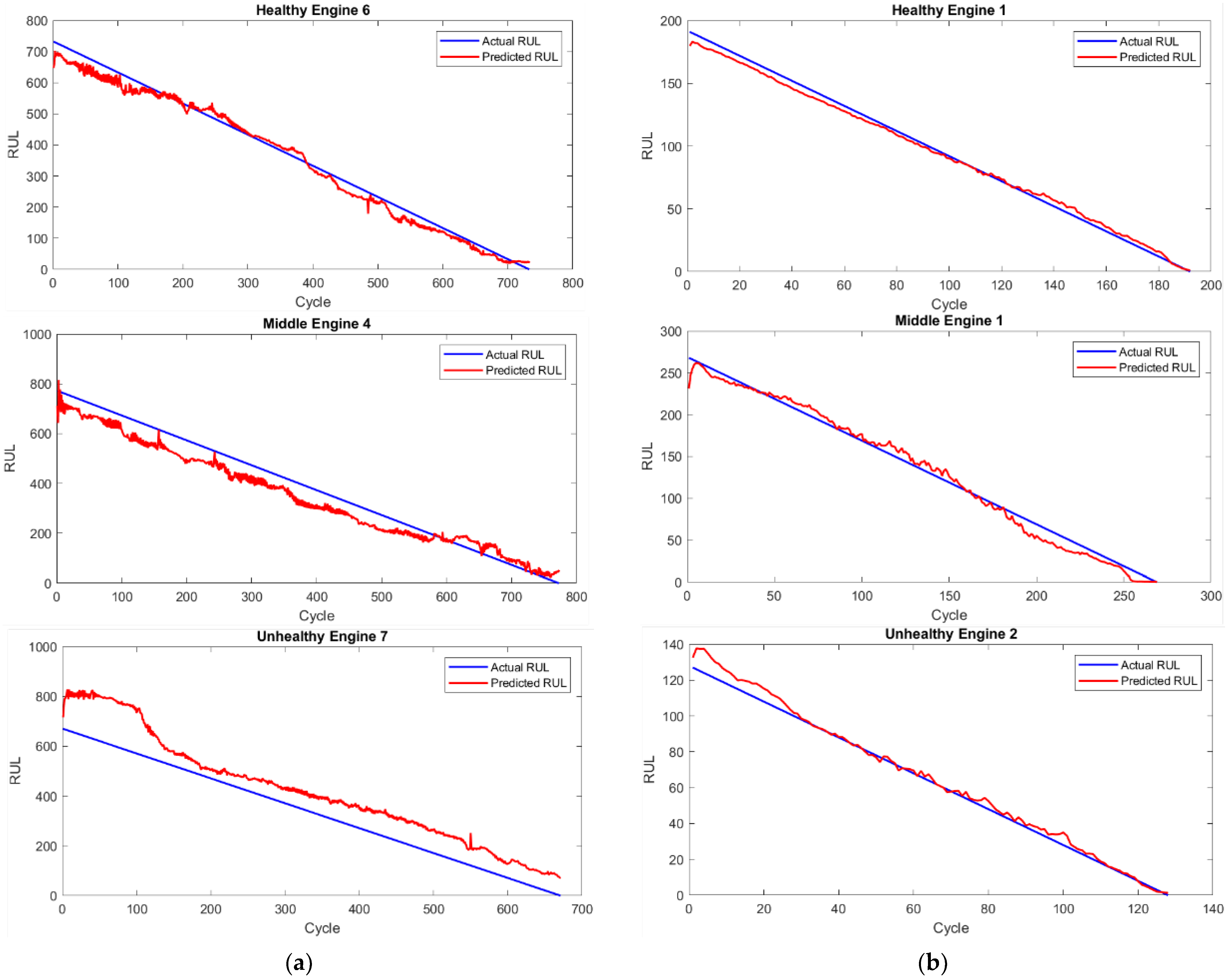
Figure 8, plots presenting actual RULs (blue lines) and predicted RULs (red lines) were presented for two datasets: real-life engine operational data (a) and CMAPSS (b), for three various engine health states.
Figure 8 presents plots comparing the actual RUL (blue lines) against the predicted RUL (red lines) for engines in three different health states across two datasets: (a) CMAPSS and (b) real-life engine operational data: Healthy: Slow decline (1000+ cycles); Unhealthy: Rapid drop (<200 cycles). CMAPSS (a) shows idealized degradation, while real data (b) exhibits stochastic fluctuations due to operational variability. Analyzing these RUL predictions, it can be concluded that the proposed neural network architecture and prediction algorithm perform better for the simulated CMAPSS dataset than for the real-life engine data. For CMAPSS, the RUL prediction lines, representing engine degradation, closely follow the actual engine life-cycle reduction, indicating high accuracy. While the predictions for real-life data show more variability, they still provide valuable prognostic information despite the inherent noise and complexity of the dataset.
Figure 9 presents examples of the engines’ RUL predictions for real-life engine operational data (a) and CMAPPS dataset (b).
Figure 9 provides illustrative examples of RUL predictions for selected engines from (a) the real-life operational data and (b) the CMAPSS dataset, showcasing the model’s performance across various engine health states. The RUL prediction results showed that while the CMAPPS dataset yielded lower RMSE values, the real-life dataset’s RUL predictions were still within an acceptable range. The Score function results suggested that while some late predictions occurred, they remained within an acceptable error margin. This highlights the practical viability of the model in industrial settings where exact failure times are difficult to ascertain, where even approximate RUL predictions can significantly aid maintenance planning.
6.4. Comparison with Other Models
This section compares the proposed model’s RUL prediction performance on the CMAPSS dataset with other state-of-the-art models from the literature. Since there are no similar complete frameworks for unsupervised engine clustering and RUL prediction validated with real-life turbofan engine operational data, the comparison focuses on the CMAPSS dataset, which is a common benchmark.
As for the unsupervised clustering, the proposed GMM methodology was compared to other types of algorithms, such as spectral clustering. The results were presented in Chapter 6.3. Spectral clustering silhouette performance was equal to 0.05 for the real-life engine operational data and 0.18 for the CMAPPS data. These were 60% and 54% lower than for the GMM clustering, which proved GMM selection legitimacy. For the K-means clustering, the average silhouette was equal to 0.16 for the CMAPPS and 0.13 for the real-life engine operational data. The results achieved were 58% lower for the CMAPPS dataset, but, for the real-life data, about 7% higher.
Still, engine RUL prediction accuracy was presented for the GMM and spectral clustering methods. The comparison is presented in
Table 3.
Comparing K-means to spectral clustering, it might be deduced that although the first one is a very popular clustering method, RUL prediction performance measured by RMSE, R2, Score, and Loss metrics achieved with spectral clustering is still better for both CMAPPS and real-life engine operational datasets, and all the metrics.
In addition to this, it was decided to compare the proposed model to the other engine RUL prediction methods described in the literature. Since there are no publications in which the proposed ML models are validated with the real-life turbofan engine operational data, it was decided to compare the proposed model to other existing RUL prediction models on the CMAPSS dataset.
Table 4 summarizes the results of RUL prediction performance comparison between the designed model and 12 existing deep neural networks specifically designed for aero-engine RUL prediction on the CMAPSS dataset. The bolded results highlight performance results for the proposed model and engine health states.
As far as the RMSE is concerned, the prediction error result is the lowest among the NN architectures compared. The difference ranges from 29–58%. As for the Score performance metric, the proposed model achieved the best result in all cases. The proposed model outperformed the others by up to an order of magnitude or even greater. It proves that the proposed model has a competitive advantage in RUL prediction performance on the CMAPSS dataset compared to other models. This fact confirms that the proposed NN architecture can comprehensively extract the hidden information from the data as well as detect the most trendable engine operational data features. This results in a better engine health status estimation and more accurate RUL prediction.
6.5. Limitations and Challenges
Despite its advantages, the proposed methodology has certain limitations. One challenge is the assumption of Gaussianity in the GMM clustering process. In some cases, real-world engine data may exhibit non-Gaussian characteristics, which could impact clustering accuracy. Future work could explore the integration of more flexible clustering methods, such as deep clustering or Gaussian Processes, to enhance adaptability.
Another limitation is the variability in sequence lengths in real-world datasets. Since LSTM models require fixed-length sequences, padding was applied, which introduced some noise into the RUL prediction process. More sophisticated sequence alignment techniques, such as dynamic time warping, could be considered in future implementations.
Real-world data introduced noise from sensor drift (e.g., ±2% Pt2 readings) and intermittent gaps (15% missing cycles). This degraded RMSE by 7–26 vs. CMAPSS (
Table 1). Mitigation strategies included robust autoencoders, in which denoising AEs [
27] trained with 10% Gaussian noise improved reconstruction by 18%, and outlier handling by winsorizing (5th–95th percentiles).which reduced Score function error by 22%.
Future work will integrate uncertainty quantification (e.g., Bayesian LSTMs [
34]) to flag low-confidence predictions. Similarly, zonotopic observers and neuro-fuzzy systems [
36,
37,
38] have proven effective for fault diagnosis in noisy wind turbine data, suggesting applicability to turbofan health monitoring.
6.6. Future Directions
To further enhance the methodology, several future research directions can be explored:
Online Learning and Adaptive Models: Implementing incremental learning techniques can allow the model to adapt to evolving sensor data patterns in real time, improving its applicability in dynamic industrial environments.
Transfer Learning for Generalization: Applying the trained model to diverse types of engines with minimal re-training could enhance its usability across various industrial applications.
Hybrid Clustering Approaches: Combining a GMM with other clustering techniques, such as spectral clustering or deep embedding clustering, could improve the classification accuracy for complex datasets.
Integration with Digital Twin Technologies: Embedding the predictive maintenance framework into digital twin systems could enable real-time monitoring and optimization of engine performance.
7. Summary and Conclusions
This article presented a comprehensive methodology for unsupervised classification using autoencoders and GMMs. The approach was applied to a real-world problem of classifying engine health states and predicting RUL. The methodology was implemented in MATLAB, and the results demonstrated its effectiveness.
The combination of autoencoders and GMMs provides a powerful tool for unsupervised classification and RUL prediction. The proposed methodology can be applied to other similar problems where labeled data is scarce or unavailable. Future work could explore the use of other unsupervised learning techniques and the integration of additional data sources.
This article presents a scalable, unsupervised framework for predictive maintenance, combining autoencoders, GMMs, and LSTMs. The methodology achieves state-of-the-art performance on the NASA dataset, demonstrating the viability of unsupervised learning in industrial applications. Future work will focus on real-time deployment and integration with digital twin technologies.
This article provides a detailed explanation of the algorithms, the scientific problem, the methodology, and the results, followed by a summary and conclusion. The methodology is implemented in MATLAB, and the results demonstrate the effectiveness of the approach in identifying distinct engine states and accurately predicting RUL.
In summary, the proposed framework successfully combines autoencoders and GMMs for unsupervised classification and RUL prediction, offering a scalable and effective solution for predictive maintenance. While some challenges remain, the results demonstrate the viability of unsupervised learning in industrial applications. By addressing the identified limitations and exploring future advancements, the methodology can be further refined to meet the demands of real-world engine health monitoring systems.
Author Contributions
Conceptualization, S.S. and T.L.; methodology, S.S.; software, S.S.; validation, S.S. and T.L.; formal analysis, S.S.; investigation, S.S.; resources, S.S.; data curation, S.S.; writing—original draft preparation, S.S.; writing—review and editing, T.L.; visualization, S.S.; supervision, T.L.; project administration, T.L.; funding acquisition, T.L. All authors have read and agreed to the published version of the manuscript.
Funding
This research received no external funding.
Informed Consent Statement
Informed consent was obtained from all subjects involved in the study.
Data Availability Statement
The authors have no permission to share engine data.
Conflicts of Interest
The authors declare no conflicts of interest.
Abbreviations
The following abbreviations are used in this manuscript:
| AE | Autoencoder |
| CMAPPS | Commercial Modular Aero-Propulsion System Simulation |
| CNN | Convolutional Neural Network |
| GMM | Gaussian Mixture Model |
| GVBN | Gaussian Variational Bayes Network |
| LSTM | Long Short-Term Memory |
| PCA | Principal Component Analysis |
| PdM | Predictive Maintenance |
| ReLU | Rectified Linear Unit |
| RMSE | Root Mean Square Error |
| RUL | Remaining Useful Life |
| SAL | Self-Attention Layer |
| t-SNE | t-Distributed Stochastic Neighbor Embedding |
| VAEs | Variational Autoencoders |
References
- Davari, N.; Veloso, B.; Ribeiro, R.P.; Gama, J. Fault Forecasting Using Data-Driven Modeling: A Case Study for Metro do Porto Data Set. In Machine Learning and Principles and Practice of Knowledge Discovery in Databases; Communications in Computer and Information Science; Springer: Cham, Switzerland, 2023; pp. 400–409. [Google Scholar] [CrossRef]
- Zhang, H.; Deng, Y.; Chen, F.; Luo, Y.; Xiao, X.; Lu, N.; Liu, Y.; Deng, Y. Fatigue Life Prediction for Orthotropic Steel Bridge Decks welds Using a Gaussian Variational Bayes Network and Small Sample Experimental Data. Reliab. Eng. Syst. Saf. 2025, 264, 111406. [Google Scholar] [CrossRef]
- Mobley, R.K. Predictive maintenance techniques. In An Introduction to Predictive Maintenance, 2nd ed.; Butterworth-Heinemann: Oxford, UK, 2002; pp. 99–113. [Google Scholar] [CrossRef]
- Ran, Y.; Zhou, X.; Lin, P.; Wen, Y.; Deng, R. A Survey of Predictive Maintenance: Systems, Purposes and Approaches. arXiv 2019, arXiv:1912.07383. [Google Scholar]
- Kingma, D.P.; Ba, J.L. Adam: A method for stochastic optimization. arXiv 2014, arXiv:1412.6980. [Google Scholar]
- Sun, X.; Zhang, T.; Xu, J.; Zhang, H.; Kang, H.; Shen, Y.; Chen, Q. Energy efficiency-driven mobile base station deployment strategy for shopping malls using modified improved differential evolution algorithm. Appl. Intell. 2022, 53, 1233–1253. [Google Scholar] [CrossRef]
- Popov, S.; Saa, O.; Finardi, P. Equilibria in the tangle. Comput. Ind. Eng. 2019, 136, 160–172. [Google Scholar] [CrossRef]
- Thill, M.; Konen, W.; Wang, H.; Bäck, T. Temporal convolutional autoencoder for unsupervised anomaly detection in time series. Appl. Soft Comput. 2021, 112, 107751. [Google Scholar] [CrossRef]
- Ribeiro, R.P.; Mastelini, S.M.; Davari, N.; Aminian, E.; Veloso, B.; Gama, J. Online anomaly explanation: A case study on predictive maintenance. In Machine Learning and Principles and Practice of Knowledge Discovery in Databases; Communications in Computer and Information Science; Springer: Cham, Switzerland, 2023; pp. 383–399. [Google Scholar] [CrossRef]
- Szrama, S. Turbofan engine health status prediction with neural network pattern recognition and automated feature engineering. Aircr. Eng. Aerosp. Technol. 2024, 96, 19–26. [Google Scholar] [CrossRef]
- Szrama, S.; Szymański, G.; Mokrzan, D. Aircraft propulsion health status prognostics and prediction. Adv. Sci. Technol. Res. J. 2025, 19, 321–335. [Google Scholar] [CrossRef] [PubMed]
- Van Den Oord, A.; Dieleman, S.; Zen, H.; Simonyan, K.; Vinyals, O.; Graves, A.; Kalchbrenner, N.; Senior, A.; Kavukcuoglu, K. WaveNet: A generative model for raw audio. arXiv 2016, arXiv:1609.03499. [Google Scholar]
- Choi, K.; Yi, J.; Park, C.; Yoon, S. Deep Learning for Anomaly Detection in Time-Series Data: Review, analysis, and guidelines. IEEE Access 2021, 9, 120043–120065. [Google Scholar] [CrossRef]
- Darban, Z.Z.; Webb, G.I.; Pan, S.; Aggarwal, C.C.; Salehi, M. Deep learning for time Series Anomaly Detection: A survey. arXiv 2022, arXiv:2211.05244. [Google Scholar]
- Davari, N.; Veloso, B.; Ribeiro, R.P.; Pereira, P.M.; Gama, J. Predictive maintenance based on anomaly detection using deep learning for air production unit in the railway industry. In Proceedings of the 2021 IEEE 8th International Conference on Data Science and Advanced Analytics (DSAA), Porto, Portugal, 6–9 October 2021; pp. 1–10. [Google Scholar] [CrossRef]
- Chauhan, S.; Vig, L. Anomaly detection in ECG time signals via deep long short-term memory networks. In Proceedings of the 2015 IEEE International Conference on Data Science and Advanced Analytics (DSAA), Paris, France, 19–21 October 2015; pp. 1–7. [Google Scholar] [CrossRef]
- Li, D.; Chen, D.; Jin, B.; Shi, L.; Goh, J.; Ng, S.-K. MAD-GAN: Multivariate Anomaly Detection for Time Series Data with Generative Adversarial Networks. In Artificial Neural Networks and Machine Learning—ICANN 2019: Text and Time Series; Lecture Notes in Computer Science; Springer: Cham, Switzerland, 2019; pp. 703–716. [Google Scholar] [CrossRef]
- Qu, H.; Zhou, J.; Qin, J.; Tian, X. Anomaly detection for industrial control networks based on improved One-Class support vector machine. Int. J. Pattern Recognit. Artif. Intell. 2020, 35, 2150012. [Google Scholar] [CrossRef]
- Ribeiro, D.; Matos, L.M.; Moreira, G.; Pilastri, A.; Cortez, P. Isolation forests and deep autoencoders for industrial screw tightening anomaly detection. Computers 2022, 11, 54. [Google Scholar] [CrossRef]
- Tien, C.-W.; Huang, T.-Y.; Chen, P.-C.; Wang, J.-H. Using autoencoders for anomaly detection and transfer learning in IoT. Computers 2021, 10, 88. [Google Scholar] [CrossRef]
- Veloso, B.; Ribeiro, R.P.; Gama, J.; Pereira, P.M. The MetroPT dataset for predictive maintenance. Sci. Data 2022, 9, 764. [Google Scholar] [CrossRef] [PubMed]
- Sayah, M.; Guebli, D.; Noureddine, Z.; Masry, Z.A. Deep LSTM enhancement for RUL prediction using Gaussian mixture models. Autom. Control Comput. Sci. 2021, 55, 15–25. [Google Scholar] [CrossRef]
- Nerurkar, P.; Shirke, A.; Chandane, M.; Bhirud, S. Empirical analysis of data clustering algorithms. Procedia Comput. Sci. 2018, 125, 770–779. [Google Scholar] [CrossRef]
- Kingma, D.P.; Welling, M. Auto-Encoding variational Bayes. arXiv 2013, arXiv:1312.6114. [Google Scholar]
- Iacus, S.M.; Mercuri, L. Implementation of Lévy CARMA model in Yuima package. Comput. Stat. 2015, 30, 1111–1141. [Google Scholar] [CrossRef]
- Zhong, Z.; Zhao, Y.; Yang, A.; Zhang, H.; Qiao, D.; Zhang, Z. Industrial Robot Vibration Anomaly Detection based on Sliding Window One-Dimensional Convolution Autoencoder. Shock Vib. 2022, 2022, 1179192. [Google Scholar] [CrossRef]
- Langarica, S.; Núñez, F. Contrastive blind denoising autoencoder for real time denoising of industrial IoT sensor data. Eng. Appl. Artif. Intell. 2023, 120, 105838. [Google Scholar] [CrossRef]
- Vincent, P.; Larochelle, H.; Bengio, Y.; Manzagol, P.-A. Extracting and composing robust features with denoising autoencoders. In Proceedings of the 25th Annual International Conference on Machine Learning Held in Conjunction with the 2007 International Conference on Inductive Logic Programming, Helsinki, Finland, 5–9 July 2008; pp. 1096–1103. [Google Scholar] [CrossRef]
- Mohamed, A.A.; Al-Saleh, A.; Sharma, S.K.; Tejani, G.G. Zero-day exploits detection with adaptive WavePCA-Autoencoder (AWPA) adaptive hybrid exploit detection network (AHEDNet). Sci. Rep. 2025, 15, 4036. [Google Scholar] [CrossRef]
- Van Der Maaten, L.; Hinton, G. Visualizing Data using t-SNE. J. Mach. Learn. Res. 2008, 9, 2579–2605. [Google Scholar]
- Hajgató, G.; Wéber, R.; Szilágyi, B.; Tóthpál, B.; Gyires-Tóth, B.; Hős, C. PredMaX: Predictive maintenance with explainable deep convolutional autoencoders. Adv. Eng. Inform. 2022, 54, 101778. [Google Scholar] [CrossRef]
- Yu, J. Bearing performance degradation assessment using locality preserving projections and Gaussian mixture models. Mech. Syst. Signal Process. 2011, 25, 2573–2588. [Google Scholar] [CrossRef]
- Heyns, T.; Heyns, P.S.; De Villiers, J.P. Combining synchronous averaging with a Gaussian mixture model novelty detection scheme for vibration-based condition monitoring of a gearbox. Mech. Syst. Signal Process. 2012, 32, 200–215. [Google Scholar] [CrossRef]
- Nguyen, H.D.; Tran, K.P.; Thomassey, S.; Hamad, M. Forecasting and Anomaly Detection approaches using LSTM and LSTM Autoencoder techniques with the applications in supply chain management. Int. J. Inf. Manag. 2020, 57, 102282. [Google Scholar] [CrossRef]
- Shao, W.; Ge, Z.; Song, Z. Semisupervised Bayesian Gaussian mixture models for Non-Gaussian Soft Sensor. IEEE Trans. Cybern. 2019, 51, 3455–3468. [Google Scholar] [CrossRef]
- Pérez-Pérez, E.; Puig, V.; López-Estrada, F.; Valencia-Palomo, G.; Santos-Ruiz, I.; Osorio-Gordillo, G. Robust fault diagnosis of wind turbines based on MANFIS and zonotopic observers. Expert Syst. Appl. 2023, 235, 121095. [Google Scholar] [CrossRef]
- Pérez-Pérez, E.; Puig, V.; López-Estrada, F.; Valencia-Palomo, G.; Santos-Ruiz, I.; Samada, S.E. Fault detection and isolation in wind turbines based on neuro-fuzzy qLPV zonotopic observers. Mech. Syst. Signal Process. 2023, 191, 110183. [Google Scholar] [CrossRef]
- Pérez-Pérez, E.; López-Estrada, F.; Puig, V.; Valencia-Palomo, G.; Santos-Ruiz, I. Fault diagnosis in wind turbines based on ANFIS and Takagi–Sugeno interval observers. Expert Syst. Appl. 2022, 206, 117698. [Google Scholar] [CrossRef]
- Essien, A.; Giannetti, C. A deep learning model for smart manufacturing using convolutional LSTM neural network autoencoders. IEEE Trans. Ind. Inform. 2020, 16, 6069–6078. [Google Scholar] [CrossRef]
- Bai, S.; Kolter, J.Z.; Koltun, V. An empirical evaluation of generic convolutional and recurrent networks for sequence modeling. arXiv 2018, arXiv:1803.01271. [Google Scholar]
- Hochreiter, S.; Schmidhuber, J. Long Short-Term memory. Neural Comput. 1997, 9, 1735–1780. [Google Scholar] [CrossRef]
- Malhotra, P.; Ramakrishnan, A.; Anand, G.; Vig, L.; Agarwal, P.; Shroff, G. LSTM-based Encoder-Decoder for multi-sensor anomaly detection. arXiv 2016, arXiv:1607.00148. [Google Scholar]
- Elsayed, M.S.; Le-Khac, N.-A.; Dev, S.; Jurcut, A.D. Network Anomaly Detection Using LSTM Based Autoencoder. In Proceedings of the 23rd International ACM Conference on Modeling, Analysis and Simulation of Wireless and Mobile Systems, Alicante, Spain, 16–20 November 2020. [Google Scholar] [CrossRef]
- Chang, Z.; Zhang, X.; Wang, S.; Ma, S.; Ye, Y.; Gao, W. ASTM: An Attention based Spatiotemporal Model for Video Prediction Using 3D Convolutional Neural Networks. In Proceedings of the 2021 IEEE International Conference on Multimedia and Expo (ICME), Shenzhen, China, 5–9 July 2021; pp. 1–6. [Google Scholar] [CrossRef]
- Samal, K.K.R.; Babu, K.S.; Das, S.K. Temporal convolutional denoising autoencoder network for air pollution prediction with missing values. Urban Clim. 2021, 38, 100872. [Google Scholar] [CrossRef]
- Huang, Y.; Tang, Y.; VanZwieten, J. Prognostics with variational autoencoder by generative adversarial learning. IEEE Trans. Ind. Electron. 2021, 69, 856–867. [Google Scholar] [CrossRef]
- Xu, Z.; Zhang, Y.; Miao, J.; Miao, Q. Global attention mechanism based deep learning for remaining useful life prediction of aero-engine. Measurement 2023, 217, 113098. [Google Scholar] [CrossRef]
- Waters, M.; Waszczuk, P.; Ayre, R.; Dreze, A.; McGlinchey, D.; Alkali, B.; Morison, G. Vibration Anomaly Detection using Deep Autoencoders for Smart Factory. In Proceedings of the 2022 IEEE Sensors, Dallas, TX, USA, 30 October–2 November 2022; pp. 1–4. [Google Scholar] [CrossRef]
- Saucedo-Dorantes, J.J.; Arellano-Espitia, F.; Delgado-Prieto, M.; Osornio-Rios, R.A. Diagnosis methodology based on deep feature learning for fault identification in metallic, hybrid and ceramic bearings. Sensors 2021, 21, 5832. [Google Scholar] [CrossRef]
- Komorska, I.; Puchalski, A. Condition monitoring using a latent space of variational autoencoder trained only on a healthy machine. Sensors 2024, 24, 6825. [Google Scholar] [CrossRef]
- Szrama, S.; Lodygowski, T. Turbofan engine health status prediction with artificial neural network. Aviation 2024, 28, 225–234. [Google Scholar] [CrossRef]
- Szrama, S.; Lodygowski, T. Aircraft Engine Remaining Useful Life Prediction using neural networks and real-life engine operational data. Adv. Eng. Softw. 2024, 192, 103645. [Google Scholar] [CrossRef]
- Dereci, U.; Tuzkaya, G. An explainable artificial intelligence model for predictive maintenance and spare parts optimization. Supply Chain Anal. 2024, 8, 100078. [Google Scholar] [CrossRef]
- Hu, L.; Jiang, M.; Dong, J.; Liu, X.; He, Z. Interpretable Clustering: A survey. arXiv 2024, arXiv:2409.00743. [Google Scholar]
- Appice, A.; Guccione, P.; Malerba, D. Transductive hyperspectral image classification: Toward integrating spectral and relational features via an iterative ensemble system. Mach. Learn. 2016, 103, 343–375. [Google Scholar] [CrossRef]
- Jiang, Y.; Lyu, Y.; Wang, Y.; Wan, P. Fusion Network Combined With Bidirectional LSTM Network and Multiscale CNN for Remaining Useful Life Estimation. In Proceedings of the 2020 12th International Conference on Advanced Computational Intelligence (ICACI), Dali, China, 14–16 August 2020; pp. 620–627. [Google Scholar] [CrossRef]
- Ren, L.; Qin, H.; Xie, Z.; Li, B.; Xu, K. Aero-Engine remaining useful life estimation based on Multi-Head networks. IEEE Trans. Instrum. Meas. 2022, 71, 3505810. [Google Scholar] [CrossRef]
- Liu, L.; Song, X.; Zhou, Z. Aircraft engine remaining useful life estimation via a double attention-based data-driven architecture. Reliab. Eng. Syst. Saf. 2022, 221, 108330. [Google Scholar] [CrossRef]
- Zhang, J.; Jiang, Y.; Wu, S.; Li, X.; Luo, H.; Yin, S. Prediction of remaining useful life based on bidirectional gated recurrent unit with temporal self-attention mechanism. Reliab. Eng. Syst. Saf. 2022, 221, 108297. [Google Scholar] [CrossRef]
- Liao, X.; Chen, S.; Wen, P.; Zhao, S. Remaining useful life with self-attention assisted physics-informed neural network. Adv. Eng. Inform. 2023, 58, 102195. [Google Scholar] [CrossRef]
- Xia, T.; Shu, J.; Xu, Y.; Zheng, Y.; Wang, D. Multiscale similarity ensemble framework for remaining useful life prediction. Measurement 2021, 188, 110565. [Google Scholar] [CrossRef]
- Wen, L.; Su, S.; Wang, B.; Ge, J.; Gao, L.; Lin, K. A new multi-sensor fusion with hybrid Convolutional Neural Network with Wiener model for remaining useful life estimation. Eng. Appl. Artif. Intell. 2023, 126, 106934. [Google Scholar] [CrossRef]
- Zhu, Q.; Zhou, Z.; Li, Y.; Yan, R. Contrastive BILSTM-enabled health representation learning for remaining useful life prediction. Reliab. Eng. Syst. Saf. 2024, 249, 110210. [Google Scholar] [CrossRef]
- Zha, W.; Ye, Y. An aero-engine remaining useful life prediction model based on feature selection and the improved TCN. Frankl. Open 2024, 6, 100083. [Google Scholar] [CrossRef]
- Li, X.; Jiang, H.; Liu, Y.; Wang, T.; Li, Z. An integrated deep multiscale feature fusion network for aeroengine remaining useful life prediction with multisensor data. Knowl. Based Syst. 2021, 235, 107652. [Google Scholar] [CrossRef]
| Disclaimer/Publisher’s Note: The statements, opinions and data contained in all publications are solely those of the individual author(s) and contributor(s) and not of MDPI and/or the editor(s). MDPI and/or the editor(s) disclaim responsibility for any injury to people or property resulting from any ideas, methods, instructions or products referred to in the content. |
© 2025 by the authors. Licensee MDPI, Basel, Switzerland. This article is an open access article distributed under the terms and conditions of the Creative Commons Attribution (CC BY) license (https://creativecommons.org/licenses/by/4.0/).


