Dynamic Graph Neural Network for Garbage Classification Based on Multimodal Feature Fusion

Abstract

Amid the accelerating pace of global urbanization, the volume of municipal solid garbage has surged dramatically, thereby demanding more efficient and precise garbage management technologies. In this paper, we introduce a novel garbage classification approach that leverages a dynamic graph neural network based on multimodal feature fusion. Specifically, the proposed method employs an enhanced Residual Network Attention Module (RNAM) network to capture deep semantic features and utilizes CIELAB color (LAB) histograms to extract color distribution characteristics, achieving a complementary integration of multimodal information. An adaptive K-nearest neighbor algorithm is utilized to construct the dynamic graph structure, while the incorporation of a multi-head attention layer within the graph neural network facilitates the efficient aggregation of both local and global features. This design significantly enhances the model’s ability to discriminate among various garbage categories. Experimental evaluations reveal that on our self-curated KRHO dataset, all performance metrics approach 1.00, and the overall classification accuracy reaches an impressive 99.33%, surpassing existing mainstream models. Moreover, on the public TrashNet dataset, the proposed method demonstrates equally outstanding classification performance and robustness, achieving an overall accuracy of 99.49%. Additionally, hyperparameter studies indicate that the model attains optimal performance with a learning rate of 2 × 10⁻⁴, a dropout rate of 0.3, an initial neighbor count of 20, and 8 attention heads.

1. Introduction

Amid the rapid pace of global urbanization, the generation of urban municipal garbage has increased exponentially, presenting unprecedented challenges to environmental protection and resource recovery. Traditional manual garbage classification methods, burdened by inefficiencies, high costs, and susceptibility to subjective biases, are increasingly inadequate to meet the demands of modern cities for efficient and precise garbage management within the framework of sustainable development. Consequently, deep learning-based intelligent garbage classification technologies, renowned for their superior performance in feature extraction and pattern recognition, have emerged as a pivotal and challenging research focus in recent years.

Early studies primarily focused on leveraging classical convolutional neural networks and their variants to enhance feature extraction and classification performance for garbage imagery. For instance, Jin et al. enhanced the MobileNetV2 model by incorporating an attention mechanism and extended its generalization capability via transfer learning, achieving a 90.7% classification accuracy on the Huawei Cloud dataset [1]. Wang et al. fused the local feature extraction strength of ResNet with the global information capture of the Vision Transformer, further integrating Pyramid Pooling Module (PPM) and Convolutional Block Attention Module (CBAM) modules to improve both performance and accuracy in garbage classification [2]. Additionally, Lee and Yeh employed an improved Single Shot MultiBox Detector (SSD) neural network, attaining a garbage detection accuracy of approximately 87%, thereby demonstrating the potential of object detection methods in this domain [3]. Furthermore, Darwis et al. combined the deep features extracted from a 50-layer Residual Network (ResNet50) with traditional classification algorithms such as Support Vector Machine (SVM), K-Nearest Neighbors (KNN), and Random Forest, achieving a garbage classification performance of 91% [4]. Li et al. built upon a 16-layer VGG network (VGG-16) by integrating content and boundary-aware mechanisms, which elevated the accuracy to 98% [5]. Ren et al., after comparing various classical convolutional neural network models, recommended the utilization of ResNet18 [6]. Similarly, both Ma et al. and Xie et al. optimized the MobileNetV2 architecture, each reporting classification accuracies exceeding 98% on their respective custom garbage datasets [7,8]. Yang et al. employed a compact convolutional neural network in conjunction with an adaptive image enhancement strategy, achieving high classification accuracy on a custom garbage dataset [9]. Concurrently, Zhao et al. exploited the advanced architecture of MobileNetV3-Large by incorporating depthwise separable convolutions, inverted residual structures, lightweight attention mechanisms, and the hard_swish activation function to facilitate deep recognition of garbage images, attaining an accuracy of 81% [10]. Qin et al. enhanced Inception V3 and integrated multi-source data, which resulted in a 4.80% improvement in classification accuracy on a real-world collected dataset [11]. Additionally, Li et al. introduced feature fusion and depthwise separable convolutions into an improved ResNet-50, achieving an accuracy of 94.13% on the TrashNet dataset [12].

While the aforementioned methods based on conventional convolutional neural network architectures have achieved remarkable success, challenges such as complex backgrounds, multi-label scenarios, and fine-grained classification in garbage images persist. To address these issues, some researchers have started exploring hybrid model designs to fully leverage the complementary advantages of diverse models. In this context, Goel et al. developed the Selective Enhanced Feature Weighted Attention Module (SEFWaM) framework, which employs transfer learning and algorithm fusion to achieve a 94.2% accuracy on the Trashnet 2.0 dataset [13]. Wu et al. utilized the Vision Transformer (ViT-B/16) in combination with an innovative asymmetric loss function, resulting in an identification accuracy exceeding 92.36% on a self-collected dataset, thereby significantly enhancing garbage data classification performance [14]. Kumar Lilhore et al. proposed a convolutional neural network (CNN) hybrid model that integrates Bidirectional Long Short-Term Memory (Bi-LSTM) with transfer learning, achieving a classification accuracy of 96.78% on the TrashNet dataset [15]. Jain and Kumar adopted the EfficientNetB3 model for fine-grained classification of garbage bags, paper bags, and plastic bags, reaching an impressive accuracy of 97% [16]. Wang et al. improved the overall discriminative power of their model by fusing the local features extracted by ResNet with the global information captured by the Vision Transformer, achieving an accuracy of 96.54% [17]. Hossen et al. introduced the Garbage Classifier Deep Neural Network (GCDN-Net) deep neural network model, which demonstrated excellent performance in both single-label and multi-label classification of urban recyclable garbage [18]. Finally, Yang et al. realized complementary model strengths by integrating ResNet, MobileNetV2, and You Only Look Once version 5 (YOLOv5), achieving an image classification accuracy of 98% [19].

To further enhance the model’s feature aggregation and information propagation efficiency, researchers have embarked on new explorations in network architecture and attention mechanisms. Wang et al. augmented the Inception-V3 framework with Inverted Bottleneck and Contextual Transformer modules, thereby bolstering the model’s capability to manage complex backgrounds [20]. Shang et al. optimized the structure of ShuffleNet V2 and integrated it with the MobileViT model to improve cross-channel information exchange, which in turn elevated garbage classification accuracy [21]. Furthermore, Wang et al. introduced the Coordinate Attention (CA) mechanism into the YOLOv5 framework, complemented by data augmentation and adversarial sample generation, which significantly improved the recognition accuracy of garbage images [22]. Yu et al. embedded multiple attention mechanisms within the YOLOv8 architecture and systematically assessed the impact of each module on overall performance [23]. In addition, Yan et al. developed an automated garbage classification system based on an enhanced YOLOv5, achieving further gains in detection precision through structural optimization [24].

To further enhance model robustness and generalization in complex scenarios, several studies have incorporated advanced optimization algorithms, dynamic construction strategies, and ensemble methods. Yulita et al. generated image embeddings using Inception V3 and combined them with Extreme Gradient Boosting (XGBoost v1.6.2) to realize efficient classification [25]. Moreover, Wandre et al. explored an ensemble approach that integrated graph neural networks and recurrent neural networks based on feature extraction from VGG16 and ResNet50, effectively capturing the spatiotemporal characteristics of plastic garbage and achieving a classification accuracy of 81% [26]. Lin et al. proposed a Dual-Branch Binarized Neural Network (DBBNN) that enhances garbage classification efficiency by refining both the network architecture and the loss function [27]. Zucai et al. and Wang and Wen. conducted targeted optimizations on Inception V3 and YOLOv8, respectively [28,29]. Zhou et al. assembled a comprehensive dataset comprising 15,000 images and applied YOLOv8 to achieve a recognition accuracy of 90% [30]. Liang and Guan introduced a novel FConvNet by integrating convolutions to augment spatial correlation [31]. Furthermore, Li et al. developed a multi-subnetwork architecture by fusing Deconvolutional Single Shot Detector (DSSD), YOLOv4, and Faster Region-based Convolutional Neural Network (Faster-RCNN), and cascade classifiers [32], while Gupta et al. achieved a detection accuracy of 98.5% on underwater images using an enhanced YOLOv8 [33]. Ma et al. further advanced the field by improving SSD and the feature fusion module, replacing VGG16 with ResNet-101 and, thereby, surpassing the performance of several existing object detection algorithms [34].

However, when confronted with the complexities and variabilities of real-world scenarios, single-model approaches or static feature extraction techniques still exhibit deficiencies in both generalization and real-time performance. Traditional feature extraction and fusion strategies often fail to fully capture the complementary information across different modalities, thereby limiting their effectiveness in handling complex backgrounds and fine-grained distinctions. Moreover, most attention mechanisms rely on static designs that are poorly equipped to adapt to dynamic changes in data distribution, which in turn undermines the model’s generalization capabilities in small-sample and extreme scenarios. Additionally, the majority of existing research continues to depend on conventional convolutional neural network architectures, missing opportunities to exploit the inter-sample relational information—most notably, the latent advantages of graph neural networks (GNNs) remain largely unexplored in the realm of garbage classification. To address these challenges, this paper proposes an innovative garbage classification method, with its primary contributions including the following:

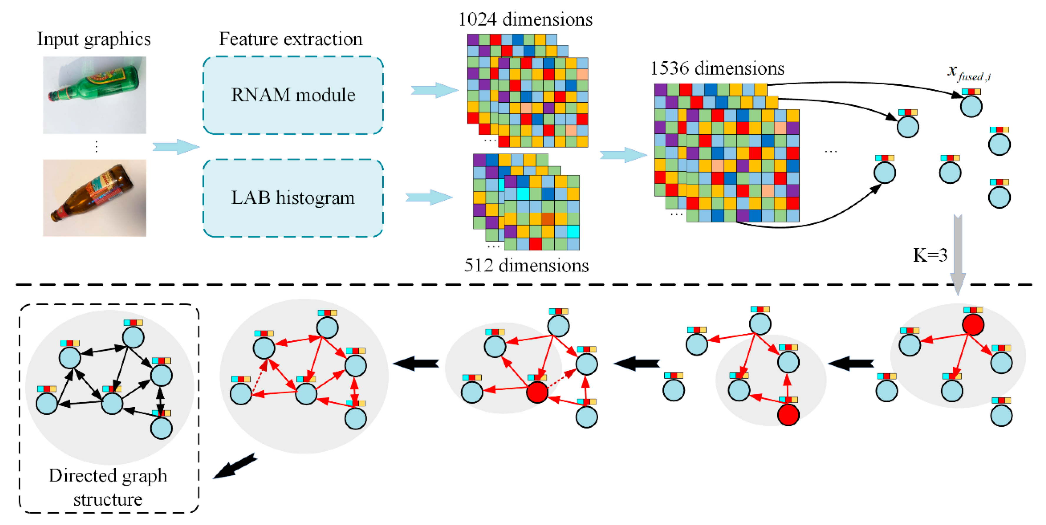
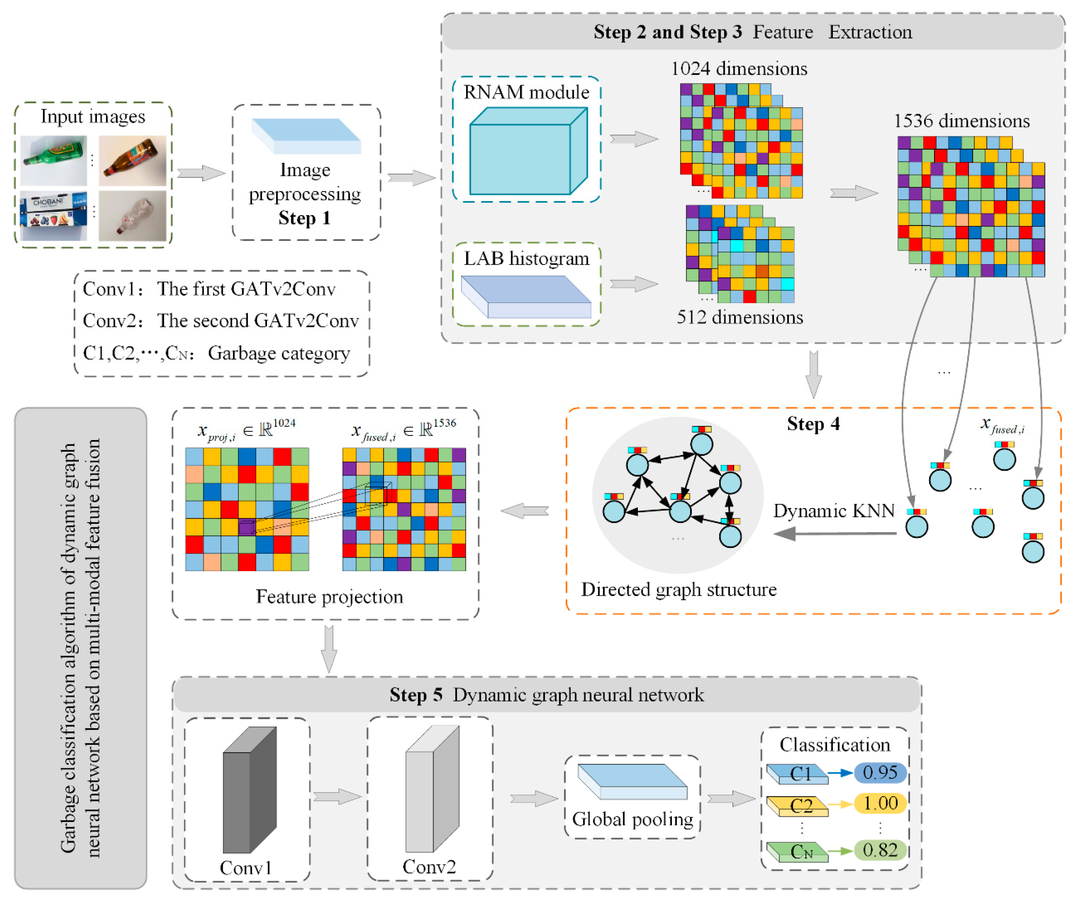
Multimodal Feature Fusion: An enhanced RNAM network model is employed to extract deep semantic features, while LAB histograms are utilized to capture color distribution information. This complementary integration of diverse modalities effectively bolsters the discriminative power of the feature representation.

Dynamic Graph Construction: Based on the fused features, a graph structure is constructed using a k-nearest neighbor algorithm. The value of k is dynamically adjusted to ensure the coherence and validity of the graph structure across varying batches, thereby effectively capturing local neighborhood relationships.

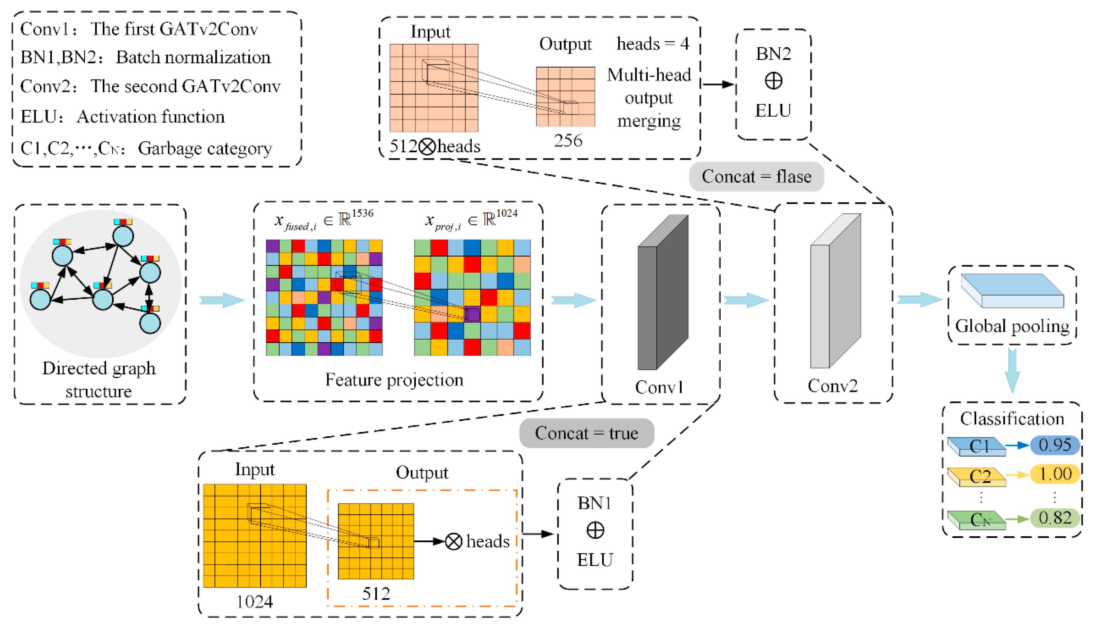
Dynamic Graph Neural Network Design: A Graph Attention Network v2 Convolution (GATv2Conv) layer is integrated into the graph structure, leveraging multi-head attention to adaptively aggregate neighborhood information. Concurrently, feature projection, batch normalization, and dropout are employed to alleviate the issue of heterogeneous feature scale mismatches, thereby effectively capturing both local and global relational features to further enhance the model’s capability for garbage image recognition.

The remainder of this paper is organized as follows. In Section 2, we provide an in-depth discussion of the multimodal feature fusion strategy for image preprocessing and feature enhancement. Section 3 elaborates on the graph construction process and details the implementation of the dynamic graph neural network. In Section 4, the design of the loss function and the corresponding optimization strategies are presented. Section 5 introduces and discusses the experimental results, and finally, Section 6 summarizes the main contributions of this work and outlines potential future research directions.

2. Multimodal Feature Fusion for Image Preprocessing and Feature Enhancement

2.1. Image Preprocessing

In the process of preprocessing and augmenting garbage images, various random transformations were applied to the images in the training set to diversify the scenes encountered during model training, enhance its generalization across different distributions, and effectively mitigate the risk of overfitting. The implemented code encompasses the following data augmentation operations: adjustments of brightness, contrast, saturation, and hue; random grayscaling; Gaussian blurring; random rotations; as well as random horizontal and vertical flipping.

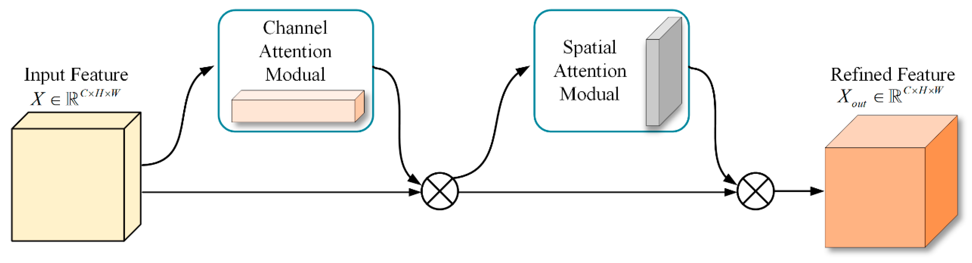
2.2. Attention Module

The attention module comprises two components, channel attention and spatial attention, which are designed to enhance feature representations along the channel and spatial dimensions, respectively. As illustrated in Figure 1, this schematic depicts the attention module architecture utilized in our study.

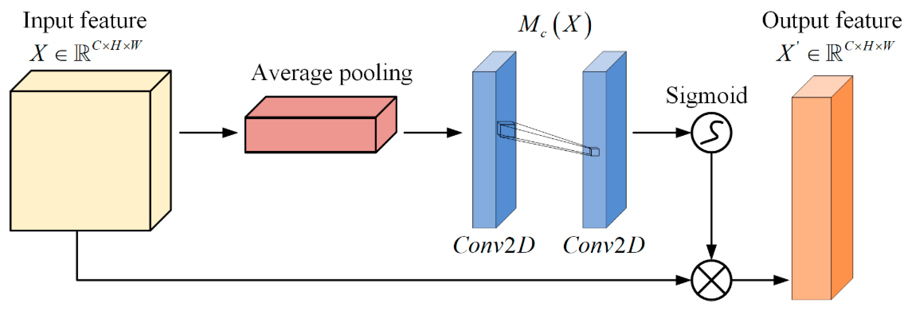
Channel attention enables the network to learn which channels are most discriminative based on the global responses of each channel, thereby enhancing these channels while suppressing less informative ones. Unlike the channel attention module in CBAM [35], which employs both average and max pooling, we exclusively utilize average pooling. The rationale is that the global feature distribution information provided by average pooling is entirely sufficient for effective channel attention learning and helps to avoid neglecting other crucial information due to local extreme values. Global average pooling:

$$F_{avg}\left[c\right]={\displaystyle \frac{1}{H\times W}}{\displaystyle \sum _{x-1}^H{\displaystyle \sum _{y-1}^{W}X\left[c,x,y\right]}}$$

(1)

Here, $X\in {\mathbb{R}}^{C\times H\times W}$ represents the input feature map, and a global average is computed for each channel to yield the vector ${\mathbb{R}}^C$.

Fully Connected Layers:

$$M_c\left(X\right)=\sigma \left(Conv2D\left(\delta \left(Conv2D\left(F_{avg}\right)\right)\right)\right)$$

(2)

Here, $\delta$ denotes the ReLU activation function, $\sigma$ represents the Sigmoid activation function, and $Conv2D\left(F_{avg}\right)$ corresponds to a fully connected layer that outputs the channel attention.

Element-wise Multiplication:

$$X^{\prime }=X\otimes M_c\left(X\right)$$

(3)

Here, $M_c\left(X\right)\in {\mathbb{R}}^{C\times 1\times 1}$ corresponds to the channel-wise weighting, while $X^{\prime }\in {\mathbb{R}}^{C\times H\times W}$ represents the channel-enhanced features. The structure of our channel attention module is depicted in Figure 2.

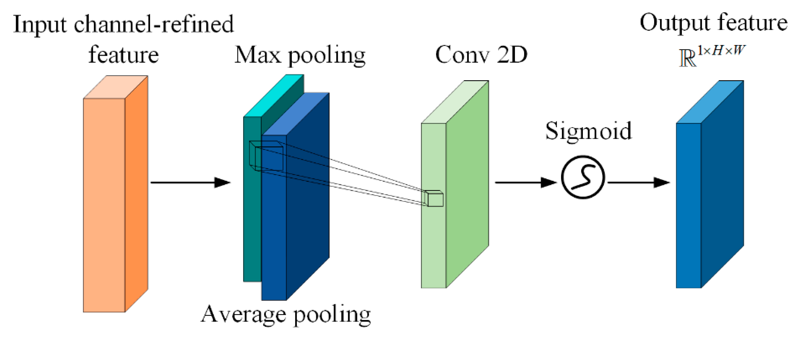
Spatial attention further weights the internal pixel positions within each channel, guiding the network to focus on regions of significant relevance. We adopt the spatial attention module from CBAM because spatial information exhibits strong local distinctiveness. The combination of max pooling and average pooling more comprehensively captures the fine-grained variations in key regions, thereby enhancing the model’s sensitivity and accuracy in localizing critical spatial features.

Max Pooling and Average Pooling:

$$X_{cat}=\left[\max \left(X^{\prime },\dim =1\right),mean\left(X^{\prime },\dim =1\right)\right]\in {\mathbb{R}}^{2\times H\times W}$$

(4)

Specifically for $X^{\prime }$, max pooling and average pooling are each applied along the channel dimension to obtain ${\mathbb{R}}^{1\times H\times W}$, which are then concatenated along the channel dimension to yield $2\times H\times W$.

Convolution-Based Spatial Attention Learning:

$$M_s\left(X^{\prime }\right)=\sigma \left(Conv2D_{7\times 7}\left(X_{cat}\right)\right)$$

(5)

The output, ${\mathbb{R}}^{1\times H\times W}$, denotes the importance of each spatial location.

Element-wise Multiplication:

$$X_{out}=X^{\prime }\otimes M_s\left(X^{\prime }\right)$$

(6)

Here, $X_{out}\in {\mathbb{R}}^{C\times H\times W}$ is the final feature map enhanced along both the channel and spatial dimensions. The structure of our spatial attention module is illustrated in Figure 3.

2.3. RNAM

A typical residual block comprises two convolution operations, batch normalization, and activation function processing. By employing a skip connection to add the input features to the transformed features, it effectively alleviates the vanishing gradient problem as the network depth increases. The overall structure can be represented as follows:

$$y=\sigma \left(x+Conv2D_2\left(\delta \left(BN\left(Conv2D_1\left(x\right)\right)\right)\right)\right)$$

(7)

Here, $x\in {\mathbb{R}}^{C\times H\times W}$ denotes the input feature map. $Conv2D_1$ and $Conv2D_2$ represent the two convolution operations, and BN stands for batch normalization. $\delta$ and $\sigma$ are the ReLU activation functions. By stacking multiple residual blocks, higher-order features ${\mathbb{R}}^{2048\times H^{\prime }\times W^{\prime }}$ can be obtained.

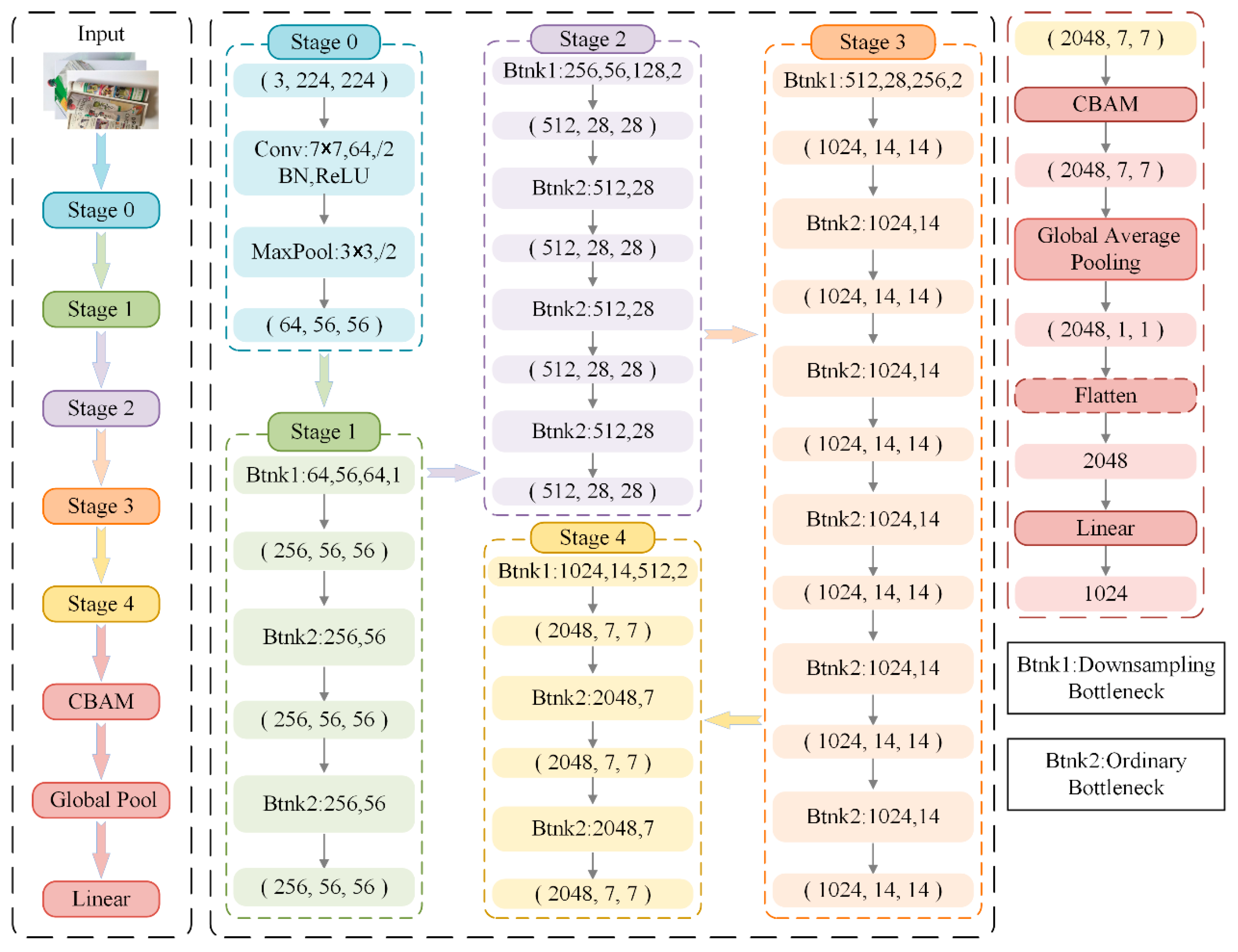
The classical ResNet50 architecture can be structurally divided into three stages. In the initial feature extraction stage, a 7 × 7 convolution kernel with a stride of 2 is employed to perform preliminary feature extraction, quickly reducing the spatial resolution. A subsequent max pooling layer with a kernel size of 3 × 3 and a stride of 2 further diminishes the feature map dimensions, laying the groundwork for the following residual units. In the multi-stage residual feature extraction phase, the network comprises four residual stages, each constructed from multiple stacked Bottleneck residual units. The first Bottleneck unit in each stage performs downsampling of the feature map, while the number of channels increases stage by stage to enhance the representational capacity. Specifically, Stage 1 contains three residual units; Stage 2 contains four; Stage 3 contains six; and Stage 4 contains three, culminating in 2048 channels in the final stage. Within these stages, the convolutional layers, batch normalization (BN), and ReLU activation functions collectively form the core feature extraction backbone of ResNet50.

The last stage employs global average pooling and a fully connected (FC) layer. While this configuration effectively reduces feature dimensionality, it struggles to adequately focus on critical regions and channels within the feature maps. To address these shortcomings, we introduce an innovative convolutional attention module and a customized global pooling architecture to replace the original fully connected layer, thereby enhancing the model’s ability to attend to crucial feature regions and improving both classification accuracy and generalization. Finally, the feature map $X_{out}$ produced by the convolutional attention module undergoes global average pooling to yield ${\mathbb{R}}^C$, which is then reduced in dimensionality via a linear layer:

$$x_{cnn}=\mathrm{Re}LU\left(BN\left(W_{proj}GAP\left(X_{out}\right)+b\right)\right)$$

(8)

Here, $GAP\left(X_{out}\right)$ converts ${\mathbb{R}}^{C\times H\times W}$ to ${\mathbb{R}}^C$, $W_{proj}\in {\mathbb{R}}^{d_{cnn}\times C}$ reduces the dimensionality from 2048 to 1024, and $x_{cnn}\in {\mathbb{R}}^{1024}$ serves as the final CNN representation. The detailed network structure of our improved RNAM is presented in Figure 4.

2.4. Color Histogram Features

To preserve global color distribution information and supplement the color cues that a CNN might otherwise overlook, especially for objects with similar appearances yet distinct coloration, we compute a 3D histogram in the LAB color space:

$$Hist\left[d_1,d_2,d_3\right]=\left|\left\{\left(x,y\right)\left|L\left(x,y\right)\in B_{d_1},\right.A\left(x,y\right)\in B_{d_2},B\left(x,y\right)\in B_{d_3}\right\}\right|$$

(9)

Here, $L$, $A$, and $B$ denote the three channels in the LAB color space. Each channel is divided into eight intervals, where $\left(d_1,d_2,d_3\right)$ indicates the corresponding $bin$ index is indicated, and the total number of counting bins is $8\times 8\times 8=512$.

Next, normalization is performed as follows:

$$His{t}_{norm}\left[d_1,d_2,d_3\right]={\displaystyle \frac{Hist\left[d_1,d_2,d_3\right]}{{\displaystyle {\sum }_{i,j,k}Hist\left[i,j,k\right]}}}$$

(10)

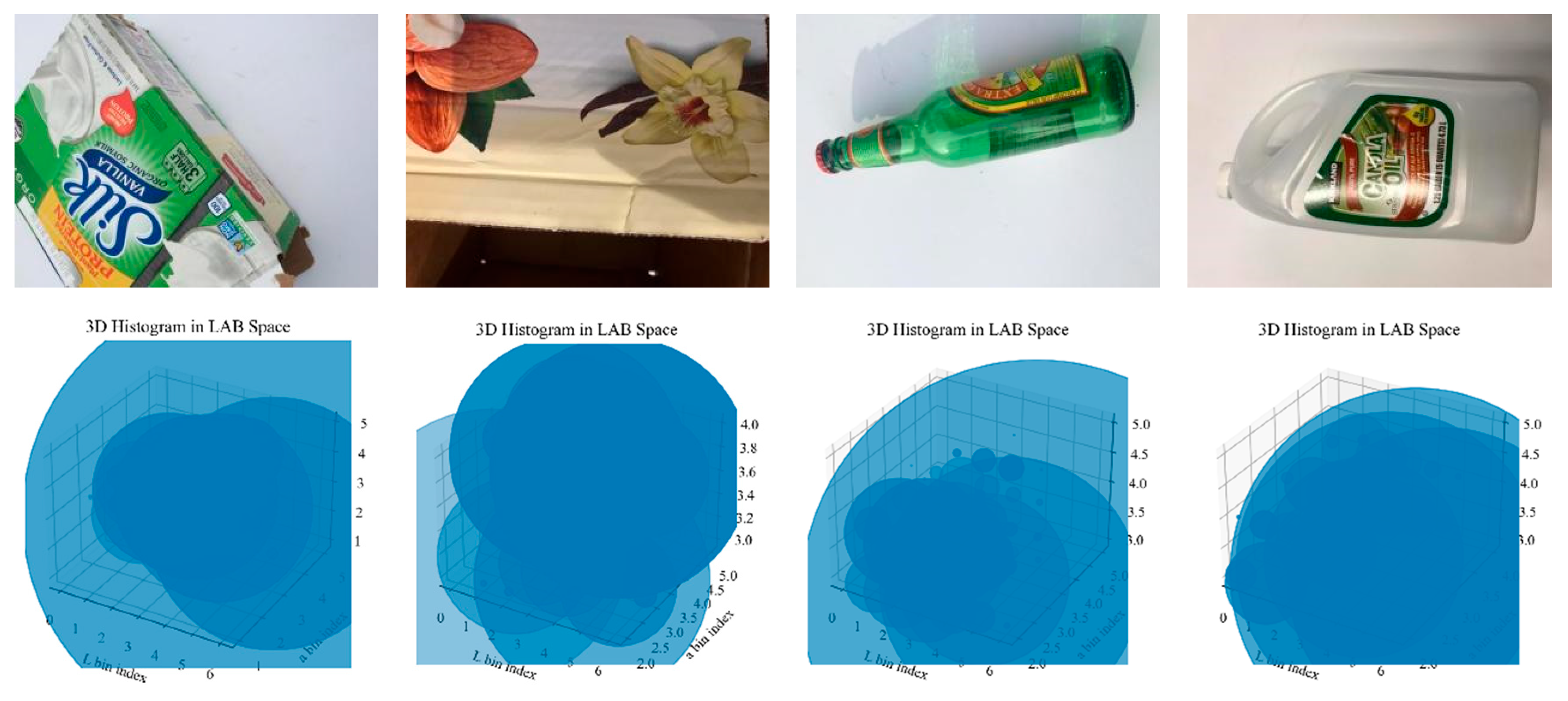
The resulting features preserve overall color distribution and complement the texture and semantic features extracted by the CNN. As illustrated in Figure 5, the upper row presents our original garbage images, and the lower row shows the 3D histograms in LAB color space. From these visualizations, it is evident that each image contains several aggregation regions in the LAB color space. The position, shape, and size of these regions vividly reflect the image’s primary brightness and chromaticity features. Taking the third image as an example, the main subject is a green bottle with a small area of colorful labeling. Most pixels are distributed near negative values on the a axis, indicating green; some pixels appear at positive values on the b axis, denoting a greenish-yellow region. Meanwhile, the L axis predominantly signifies illumination intensity and generally exhibits a lower distribution. The histogram displays one or two relatively concentrated clusters, suggesting that the color is fairly uniform and predominantly green.

2.5. Multimodal Feature Fusion

After data augmentation and CNN-based extraction, the resulting 1024-dimensional features are concatenated with the 512-dimensional features obtained via LAB histogram calculation and normalization, forming a 1536-dimensional feature vector. This concatenation operation retains the strengths of both feature sets, encompassing deep semantic information as well as statistical color information, thereby enabling the subsequent graph neural network to build and classify graphs using a richer feature representation.

3. Graph Construction and Dynamic Graph Neural Network

3.1. Dynamic KNN Graph Construction

Each image not only possesses a 1024-dimensional feature vector $x_{cnn,i}$ extracted by the CNN but also includes a 512-dimensional color histogram feature $x_{hist,i}$. These two sets of features are concatenated to form the node feature $x_{fused,i}$ representation:

$$x_{fused,i}=\left[x_{cnn,i},x_{hist,i}\right]\in {\mathbb{R}}^{1536}$$

(11)

For a batch of N images, we obtain N node features, denoted as ${\left\{x_{fused,i}\right\}}_{i-1}^N$. Then, using the Euclidean distance, the distance $dist\left(i,j\right)$ between each node $i$ and every other node $j$ ($i\ne j$) is computed as follows:

$$dist\left(i,j\right)={‖x_{fused,i}-x_{fused,j}‖}_2$$

(12)

Next, all distance values are sorted, and the top k closest nodes are dynamically selected as neighbors for node $i$. When the total number of samples is limited, the actual number of neighbors is dynamically adjusted to $min(k,N-1)$ to ensure the soundness of the graph structure. Finally, a directed edge marked as $\left(i,j\right)$ is recorded in the adjacency matrix, and a two-dimensional tensor is constructed to describe the index relationships between the starting and ending nodes of each edge in the graph, thus enabling adaptive graph construction. Assuming that k is set to 3—allowing up to three nodes to be adaptively chosen as neighbors—the detailed process of dynamic KNN graph construction is illustrated in Figure 6.

As illustrated in the dynamic example in Figure 6, for the red node, within the pre-defined neighborhood, the distance between the red node and its surrounding nodes is first computed $dist\left(i,j\right)$. Based on these distances, up to three of the closest nodes are selected to form the initial candidate neighborhood set. Within this candidate set, a directed edge is established between the red node and each candidate, with the edge orientation indicating that it points from the red node toward the nearest target node. Moreover, when the red node and a candidate node mutually fall within each other’s neighborhoods, it indicates that these two nodes exhibit a high degree of similarity in the feature space, resulting in the formation of a bidirectional connection.

3.2. Dynamic Graph Neural Network

3.2.1. Feature Projection

Before being fed into the GNN, the concatenated feature vector is linearly mapped to $x_{fused,i}\in {\mathbb{R}}^{1536}$ 1024-dimensional space, after which batch normalization and ReLU activation are sequentially applied:

$$x_{proj,i}=\mathrm{Re}LU\left(BN\left(W_{fuse}{x}_{fused,i}+b\right)\right)$$

(13)

In the formula, $x_{proj,i}$ represents the feature vector after multimodal concatenation of the sample; $W_{fuse}$ is the weight matrix; $b$ is the bias vector; $\mathrm{Re}LU$ is the activation function; $x_{fused,i}$ is the output feature vector.

To prevent the network from becoming excessively large, feature projection is utilized to reduce the input dimensionality to the GNN. Moreover, a subsequent linear transformation is performed prior to the integration of the CNN and graph structures to facilitate a more effective fusion of the two types of features.

3.2.2. Multi-Head Graph Attention Network

Multi-head attention facilitates the capture of neighborhood features across multiple subspaces, thereby enhancing the model’s expressive capacity. For a GATv2Conv layer, assume the input dimension is $d_{in}$ and the output dimension is $d_{out}$. For node $i$ and its neighbor $N\left(i\right)$, a linear transformation is applied as follows:

$$h_i=W{x}_{proj,i}$$

(14)

Here, $W\in {\mathbb{R}}^{d_{attn}\times d_{in}}$. The attention score $e_{ij}$ is defined as follows:

$$e_{ij}=a^T\delta \left(h_i+h_j\right)$$

(15)

Here, $j\in N\left(i\right)$, $a\in {\mathbb{R}}^{d_{attn}}$ represent the learnable parameter, while $\delta$ denotes the LeakyReLU activation function; $h_i$ and $h_j$ are the projection features of node $i$ and its neighbor $j$. Subsequently, Softmax normalization is applied:

$${\alpha }_{i,j}={\displaystyle \frac{\exp \left(e_{ij}\right)}{{\displaystyle {\sum }_{k\in N\left(i\right)}\exp }\left(e_{ik}\right)}}$$

(16)

In the formula, ${\alpha }_{i,j}$ represents the normalized attention coefficient of node $j$ with respect to $i$. Finally, neighborhood aggregation is performed:

$$x_i^{\prime }=ELU\left({\displaystyle \sum _{j\in N\left(i\right)}{\alpha }_{\partial ij}{h}_j}\right)$$

(17)

In the formula, $x_i^{\prime }$ is the new feature representation of node $i$ after aggregating neighborhood information; $ELU$ represents nonlinear activation, enhancing expressive ability. When employing multiple attention heads H, each head independently learns its own set of weight parameters $W^{\left(r\right)}$ and $a^{\left(r\right)}$ and extracts partial features. If a concatenation strategy is adopted—where the outputs of all attention heads are concatenated—the final output dimensionality is $H\times d_{out}$; alternatively, if an aggregation strategy is utilized, where a weighted summation is performed, all attention head outputs are integrated into a $d_{out}$ dimensional representation.

3.3. Global Pooling

Within the graph neural network framework, to classify the entire graph, a global pooling operation is employed. Its computation is described as follows:

$$z_g=MeanPool\left({\left\{x_i^{\prime }\right\}}_{i\in V_g}\right)={\displaystyle \frac{1}{\left|V_g\right|}}{\displaystyle \sum _{i\in V_g}{x}_i^{\prime }}$$

(18)

Here, $V$ denotes the set of nodes contained within a graph or subgraph. $z_g$ is a graph-level representation vector used for subsequent whole graph classification or regression tasks.

In the context of this specific task, each image corresponds to a single node within the graph structure; consequently, the global pooling operation effectively reduces to an identity mapping on that node. To comply with the input format requirements of the graph neural network framework, batch indices are introduced to differentiate between distinct graph samples.

3.4. Classification Layer

Finally, the pooled node representations—serving as the global representation of each graph—are mapped to the target classification space via a fully connected network, and the prediction probabilities for each class are computed using the log-softmax function:

$$p_i=\log \_soft\max \left(W_2\delta \left(W_1{z}_g+b_1\right)+b_2\right)$$

(19)

In the formula, $W_1$ represents the weight matrix of the first fully connected layer; $b_1$ is the first bias vector; $W_2$ is the weight matrix of the second fully connected layer; $b_2$ is the second bias vector; $p_i$ is the category logarithmic probability vector obtained after using log-softmax.

Finally, a multilayer perceptron (MLP) is employed to map the GNN representation to the specific classification task, with training conducted using a loss function such as negative log-likelihood or cross-entropy. Figure 7 illustrates the detailed design of the dynamic graph neural network architecture. In this framework, a directed graph constructed via a dynamic KNN algorithm—with adaptive neighborhood relationships—is first subjected to feature projection for dimensionality reduction and subsequently used as input. An improved graph attention convolution module then efficiently aggregates local neighborhood information through a multi-head attention mechanism. Two stacked attention convolution layers, followed by ELU activation and normalization, enhance the model’s capacity to represent higher-order topological structures. Finally, a fully connected layer combined with a softmax classifier accomplishes the ultimate classification task.

4. Loss Function and Optimization

4.1. Negative Log Likelihood

If the network’s output log probabilities for the classes are denoted by $\log p_{i,c}$ and the true label of the sample is $y_i$, then the negative log-likelihood (NLL) loss can be formulated as

$${\tau }_{nll}=-{\displaystyle \sum _{i-1}^N\log \left(p_{i,y_i}\right)}$$

(20)

This loss function is typically used in conjunction with the log-softmax function. It is numerically equivalent to the cross-entropy loss and exhibits robust numerical stability.

4.2. AdamW Optimizer

AdamW is a widely adopted optimization algorithm in both graph neural networks (GNNs) and convolutional neural networks (CNNs). It combines the adaptive learning rate advantages of Adam with an explicit weight decay strategy for effective regularization, thereby mitigating overfitting. Its weight update formula is given by

$$w\leftarrow w-\eta \left(\widehat{g}\left(w\right)+\lambda w\right)$$

(21)

Here, $w$ represents the model parameters to be optimized; $\widehat{g}\left(w\right)$ denotes the gradient estimate from Adam after bias correction of the first and second moment estimates; $\lambda$ is the weight decay coefficient (i.e., the strength of weight regularization), corresponding to weight decay; and $\eta$ is the learning rate.

4.3. Cosine Annealing Scheduler

During model training, to enhance both convergence speed and generalization performance, we adopt a cosine annealing scheduling strategy to adjust the learning rate. The update formula is given as follows:

$${\eta }_t={\eta }_{\min }+{\displaystyle \frac{1}{2}}\left({\eta }_{\max }-{\eta }_{\min }\right)\left(1+\cos \left({\displaystyle \frac{T_{cur}}{T_{\max }}}\pi \right)\right)$$

(22)

Here, $t$ denotes the current training iteration, $T_{cur}$ represents the number of iterations already executed, and $T_{\max }$ indicates the predetermined maximum annealing cycle. This cosine annealing strategy enables the learning rate to decrease following a cosine curve during the training process, affecting a gradual decay that is conducive to fine-tuning the model in later stages. Moreover, cosine annealing can be combined with a restart mechanism, allowing for periodic reinitialization of the learning rate throughout training to further enhance model convergence.

Building upon the aforementioned studies, this work proposes a classification method based on a dynamic graph neural network model that fuses multimodal features, aimed at improving the accuracy and robustness of garbage classification. The overall logical framework is illustrated in Figure 8, and the specific steps are outlined as follows:

Step 1: Data augmentation strategies are applied to the input images, including random color jitter, grayscale transformations, Gaussian blurring, rotation, and flipping. These operations emulate variations in illumination and viewing angles encountered in real-world scenarios, thereby enhancing the model’s robustness to complex environments.

Step 2: An improved deep convolutional neural network, RNAM, is employed to extract high-level visual features from the raw images. Meanwhile, color space transformations and histogram calculations are utilized to capture the color distribution information of the images, allowing for a more comprehensive representation of the data.

Step 3: The deep visual features extracted by the RNAM network are concatenated with the LAB histogram features, effectively integrating two complementary modalities and yielding a multimodal feature vector that encompasses both global and local information.

Step 4: Based on these multimodal features, an adaptive K-nearest neighbor algorithm is used to construct a graph structure, dynamically adjusting the number of neighbors and adaptively selecting neighboring relationships among the features. This process realizes adaptive connectivity between graph nodes, capturing salient graph structural properties.

Step 5: A multi-layer graph attention network is employed to efficiently extract features from the constructed graph. By combining global average pooling and a fully connected layer to classify the resulting graph embeddings, the framework achieves precise recognition and classification of garbage images.

The complete process of the multimodal feature fusion-based dynamic graph neural network model classification algorithm is provided in Algorithm 1:

Algorithm 1: Garbage classification algorithm of dynamic graph neural network based on multi-modal feature fusion

Input: $D_{train}={\left\{\left(x_i,y_i\right)\right\}}_{i=1}^{N_{train}}$, $D_{test}={\left\{\left(x_i,y_i\right)\right\}}_{i=1}^{N_{test}}$, $\theta =\left\{bs,k,T,\alpha ,h,p,\lambda \right\}$

where $bs$: batch size, $k$: initial number of neighbors, $T$: number of epochs, $\alpha$: learning rate, $h$: number of heads, $p$: dropout probability, $\lambda$: weight decay

Output: Best test accuracy $A_{best}$

Define: $A\left(x\right)$: augmentation

$CNN\left(x\right)$: RNAM for deep feature extraction

$Hist\left(x\right)$: LAB histogram features

$F=CNN\left(A\left(x\right)\right)\oplus Hist\left(x\right)$: fused features ($\oplus$ denotes concatenation)

$E=\mathit{Dynamic}KNN\left(F,k^{\prime }\right)with k^{\prime }=\min \left(k,N-1\right)$

$G=\left(F,E,y\right)$: graph data

$GNN\left(G\right)$: graph neural network (based on GATv2Conv)

$L=CE\left(\widehat{y},y\right)$: cross-entropy loss

Process: 1. Feature Extraction:

For each sample $x$ in $D$:

$x^{\prime }\leftarrow A\left(x\right)$

$x_{img}\leftarrow CNN\left(x^{\prime }\right)$

$x_{hist}\leftarrow Hist\left(x\right)$

$F\leftarrow x_{img}\oplus x_{hist}$

2. Graph Construction:

For each mini-batch (size N):

$k^{\prime }\leftarrow \min \left(k,N-1\right)$

$E\leftarrow \mathit{Dynamic}KNN\left(F,k^{\prime }\right)$

$G\leftarrow \left(F,E,y\right)$

3. Graph Classification:

$\widehat{y}\leftarrow GNN\left(G\right)$ (via global pooling and FC layer with log-softmax)

4. Training And Evaluation;

$A_{best}\leftarrow 0$

For $t=1$ to $T$ do

Training:

For each mini-batch in $D_{train}$:

(i) Extract $F$ and construct $G$

(ii) $\widehat{y}\leftarrow GNN\left(G\right)$

(iii) $L\leftarrow CE\left(\widehat{y},y\right)$

(iv) Update parameters (AdamW and gradient clipping)

Testing:

For each mini-batch in $D_{test}$:

Repeat (i)–(ii), accumulate accuracy $A_{test}$

If $A_{test}>A_{best}$ then

Set $A_{best}\leftarrow A_{test}$ and save the model

Update $\alpha \leftarrow \mathrm{Cos}ineAnnealing\left(\alpha \right)$

end for

Return: $A_{best}$

5. Experiments

5.1. Dataset Description

The proposed algorithm is experimentally validated on both our self-constructed kitchen garbage, recyclable garbage, hazardous garbage, and other garbage (KRHO) dataset and the public TrashNet [36] dataset, thereby demonstrating its superiority. The KRHO dataset was primarily gathered through web searches and web crawlers, followed by multiple rounds of meticulous data cleaning. It comprises four categories: kitchen garbage, recyclable garbage, hazardous garbage, and other garbage. Specifically, there are 24 subcategories of kitchen garbage with a total of 3512 images; 24 subcategories of recyclable garbage with 3414 images; 7 subcategories of hazardous garbage with 888 images; and 15 subcategories of other garbage with 1308 images, amounting to 9122 images overall. To ensure fairness in the experimental evaluation, the dataset is partitioned into training and testing sets in an 8:2 ratio. For instance, as detailed in

Table 1. Hazardous garbage partitioning example.

Category	Name	Number	Training Set	Test Set
Hazardous garbage	Lamp	99	79	20
	Battery	152	122	30
	Glue	48	39	9
	Button battery	104	83	21
	Solar cell	68	54	14
	Storage battery	129	103	26
	Pharmaceutical packaging	288	230	58
Addition		888	710	178

, using hazardous garbage as an example, the images from the seven subcategories of hazardous garbage are merged into the respective training and testing sets, resulting in 710 training images and 178 testing images. Applying the same partitioning strategy to the remaining three categories yields a final split of 7310 images for training and 1812 images for testing. Although the original resolutions of the images vary, they are uniformly resized to 224 × 224 pixels during preprocessing to align with the input requirements of our model. Detailed information regarding the self-constructed KRHO dataset is provided in Figure 9.

The public TrashNet dataset comprises 2527 RGB images spanning six garbage categories, with the following distribution: 501 images of glass, 594 of paper, 403 of cardboard, 482 of plastic, 410 of metal, and 137 of general garbage. In our experiments, we selected only four categories—glass, paper, cardboard, and plastic—for evaluation. The processing approach is identical to that used for our self-constructed KRHO dataset: each category is split into training and testing sets in an 8:2 ratio, and all images are uniformly resized to 224 × 224 pixels prior to input.

5.2. Experimental Details

During training, several hyperparameters utilized by the model are listed in

Table 2. Model hyperparameter settings.

Symbols	Parameter	Symbols	Parameter
Batch_size	64	Epochs	100
Num_workers	8	Lr	2 × 10−4
Knn_k	20	Epochs	100
Cnn_feat_dim	1024	Num_heads	8
Hist_feat_dim	512	Dropout	0.3
Num_classes	4	Weight_decay	1 × 10−4

. The computer configuration used in this study is as follows: 13th Generation Intel^® Core™ i5-13400F @ 2.50 GHz, 32 GB of RAM, and an NVIDIA GeForce RTX 4060 Ti GPU manufactured in Gainesville, FL, USA. The network model was implemented using CUDA 12.4, Python 3.11.11, and the PyTorch 2.6.0 framework. Our network architecture and parameter configurations are detailed in

Table 3. Our proposed method structure and parameter settings.

Module	Configuration/Operation	Input Size	Output Size
Data Preprocessing	Data enhancement	Graphics 224 × 224 × 3	Graphics 224 × 224 × 3
			Histogram 512-D
Feature Extraction	CNN	Graphics 224 × 224 × 3	Feature 1024-D
Feature Fusion	CNN feature and LAB	Feature 1024-D	Feature 1536-D
		Histogram 512-D
Graph Construction	Dynamic KNN	Fusion feature N × 1536	-
Dynamic GNN	GATv2Conv	Node feature 1536-D	Renewal feature 256-D
Classification	FC classifier	Node feature 256-D	Category prediction 4

.

5.3. Experiments and Results Analysis

5.3.1. Experiments on the Self-Constructed KRHO Dataset

To validate the effectiveness of the proposed algorithm, we first conducted comparative experiments on the self-constructed KRHO dataset against four widely used classification models: DenseNet121 [37], InceptionV3 [38], MobileNetV2 [39], and ResNet50 [40]. They were chosen because DenseNet121, InceptionV3, MobileNetV2, and ResNet50, respectively, represent four mainstream design paradigms, namely feature reuse, multi-scale extraction, lightweight, and deep residual, which can comprehensively evaluate the performance of the proposed methods under different architectures. The structural configurations of these four models are detailed in

Table 4. Structural configurations of the four baseline models.

	DenseNet121	InceptionV3	MobileNetV2	ResNet50
Backbone Network	Dense Block	Inception Module	Inverted Residual	Residual Block
Input Size	224 × 224	229 × 229	224 × 224	224 × 224
Batch_size	64	64	64	64
Lr	1 × 10−3	1 × 10−3	1 × 10−3	1 × 10−3
Dropout	0.5	0.5	0.5	0.5

, while the classification accuracy and loss trends for all five methods are illustrated in Figure 10. As shown in the accuracy and loss curves in Figure 10, our proposed method demonstrates a clear performance advantage on the KRHO dataset. It achieves a rapid increase in accuracy during the early stages of training and consistently maintains a leading position throughout the training process. Likewise, the loss curve shows a sharp initial decline and remains significantly lower than those of DenseNet121, InceptionV3, MobileNetV2, and ResNet50 throughout the entire training phase. Our method not only surpasses other architectures in terms of convergence speed and final accuracy but also exhibits smaller fluctuations on the test set, highlighting its superior feature learning capability and generalization performance for the garbage classification task.

To further demonstrate the contribution of each improvement to the network’s performance, we conducted ablation experiments assessing the effects of the attention module applied to CNN-extracted features, the use of histogram features for multimodal fusion, and the implementation of a dynamic K value. In these experiments, when employing the dynamic K strategy, K is set to 20; in contrast, when not using dynamic K, K is fixed at 10 since a fixed K of 20 can lead to graph construction issues, with the maximum fixed value being 14. The comparative numerical results of the ablation experiments are presented in

Table 5. Ablation experiment test results.

Experiment Name	Attention	Histogram Features	Dynamic K	Training Accuracy/%	Test Accuracy/%
Our Method	√	√	√	99.49	99.33
No Attention	×	√	√	99.30	98.12
No Hist	√	×	√	99.19	98.51
Fixed K	√	√	×	99.37	97.52
No Attention and No Hist and Fixed K	×	×	×	99.02	97.13

The best results are marked in bold. “√” indicates the existence of this module, “×” represents None.

. The results clearly indicate that our method, which integrates the attention mechanism, histogram feature fusion, and dynamic K selection, achieves the highest test accuracy, significantly outperforming approaches that incorporate only some of these components. Specifically, the inclusion of an attention mechanism enhances the network’s ability to focus on discriminative target regions; the fusion of histogram features further enriches the model’s feature representation; and the dynamic K strategy adaptively adjusts the classification decision boundaries, thereby effectively improving the overall performance. The synergistic effect of these components leads to the optimal performance on the test set, underscoring the critical contribution of each module to the network’s enhanced performance.

During the experimental process, to ensure fair comparison with existing methods, we employed detailed evaluation metrics including Precision, Recall, F1 Score, Accuracy, Macro Average (MA), Weighted Average (WA), and Support. Precision represents the proportion of true positive instances among all samples predicted as positive. Recall measures the proportion of actual positive instances that are correctly identified by the model. The F1 Score, defined as the harmonic mean of Precision and Recall, prevents overemphasis on a single metric by ensuring that a low value in either Precision or Recall results in a correspondingly low F1 Score. Accuracy indicates the proportion of samples that the model correctly predicts, irrespective of class. Macro Average reflects the model’s overall balance across all categories, while Weighted Average more accurately represents the model’s performance on dominant classes (those with a larger number of samples) in cases of imbalanced class distributions. Support denotes the number of true samples for each category in the test set. The computation formulas for each evaluation metric are as follows:

$$Precision={\displaystyle \frac{TP}{TP+FP}}$$

(23)

$$Recall={\displaystyle \frac{TP}{TP+FN}}$$

(24)

$$F1=2\times {\displaystyle \frac{Precision\times Recall}{Precision+Recall}}$$

(25)

$$Accuracy={\displaystyle \frac{TP+TN}{TP+TN+FP+FN}}$$

(26)

$$MA={\displaystyle \frac{1}{N}}{\displaystyle \sum _{c=1}^{N}Precisio{n}_c}$$

(27)

$$WA={\displaystyle \frac{{\displaystyle {\sum }_{c=1}^N\left(Precisio{n}_c\times Suppor{t}_c\right)}}{{\displaystyle {\sum }_{c=1}^{N}Suppor{t}_c}}}$$

(28)

Here, TP denotes true positives, i.e., instances predicted as positive where the actual label is also positive; FP denotes false positives, i.e., instances predicted as positive while the actual label is negative; FN denotes false negatives, i.e., instances predicted as negative despite the actual label being positive; and TN denotes true negatives, i.e., instances predicted as negative where the actual label is also negative.

Table 6. Evaluation report of the five models on the self-constructed KRHO dataset.

Categories/Indicators		DenseNet121	InceptionV3	MobileNetV2	ResNet50	Ours	Support
Hazardous garbage	Precision	0.95	0.95	0.83	0.89	0.99	178
	Recall	0.94	0.94	0.81	0.88	0.99
	F1	0.94	0.95	0.82	0.88	0.99
Kitchen garbage	Precision	1.00	1.00	0.98	1.00	1.00	690
	Recall	0.99	1.00	0.97	0.99	1.00
	F1	0.99	1.00	0.97	0.99	1.00
Other garbage	Precision	0.94	0.94	0.81	0.91	0.98	262
	Recall	0.92	0.93	0.72	0.81	0.98
	F1	0.93	0.93	0.76	0.85	0.98
Recyclable garbage	Precision	0.96	0.97	0.88	0.93	0.99	682
	Recall	0.98	0.98	0.93	0.98	0.99
	F1	0.97	0.97	0.90	0.95	0.99
Accuracy	-	0.97	0.97	0.90	0.95	0.99	1812
MA	Precision	0.96	0.96	0.88	0.93	0.99	1812
	Recall	0.96	0.96	0.86	0.91	0.99
	F1	0.96	0.96	0.87	0.92	0.99
WA	Precision	0.97	0.97	0.90	0.95	0.99	1812
	Recall	0.97	0.97	0.90	0.95	0.99
	F1	0.97	0.97	0.90	0.95	0.99

The best results are marked in bold.

presents the evaluation report for the five models on the self-constructed KRHO dataset.

As evidenced by the results presented in Table 6, our proposed method significantly outperforms the comparative approaches across all evaluation metrics. For example, in the case of hazardous garbage, our approach achieves a precision, recall, and F1 score of 0.99—an improvement of 4–5 percentage points over the most competitive baseline—demonstrating accurate and stable classification of challenging samples. Moreover, in the high-frequency kitchen garbage category, our method maintains a perfect precision of 1.00, while its recall and F1 scores either exceed or are on par with the highest records observed for the alternative networks. This clearly underscores the method’s robust capability in reliably detecting large volumes of everyday garbage.

Similarly, for both other garbage and recyclable garbage, our method achieved precision, recall, and F1 scores close to 0.99, clearly demonstrating enhanced generalization and robustness in discriminating among diverse garbage types. In terms of aggregate metrics, whether considering overall accuracy or summary indicators such as macro averages and weighted averages, the results further confirm that our approach excels not only in major categories but also in class recognition under imbalanced sample distributions, thereby minimizing misclassifications and omissions. This highlights its robust learning capabilities and superior classification performance in complex scenarios.

To quantitatively illustrate the accuracy and error rates of the five methods for garbage classification, we further conducted experiments using confusion matrices. The results are presented in Figure 11.

As depicted in the confusion matrices, our proposed method exhibits a markedly stronger discriminative ability across the four garbage categories. Not only are the diagonal values significantly higher, but the misclassifications are also confined to only a few sparse locations, outperforming the other four networks considerably. Specifically, between easily confused categories such as hazardous garbage and recyclable garbage, alternative models tend to incur substantial cross-category misclassifications, whereas our method nearly eliminates these errors. In the case of kitchen garbage—a category with a large number of samples—our method also maintains an exceptionally low misclassification rate, demonstrating robust feature extraction and discrimination capabilities even on highly heterogeneous data.

5.3.2. Experiments on the Public Dataset TrashNet

To comprehensively validate the generalization capability of the proposed method, we conducted rigorous experiments on the public TrashNet dataset following initial verification on our self-constructed dataset designed to simulate real-world application scenarios. Public datasets provide an objective basis for evaluating model robustness and transfer performance under varying data distributions. As shown in Figure 12, the proposed method continues to demonstrate superior classification performance on the public dataset, with both accuracy and loss metrics significantly outperforming state-of-the-art models such as DenseNet121, InceptionV3, MobileNetV2, and ResNet50. These results conclusively highlight the excellent generalization ability of our approach in diverse data environments.

To further validate the broad applicability of the proposed model algorithm, we conducted a more in-depth evaluation on the public TrashNet dataset. The evaluation results are presented in

Table 7. Evaluation report of the five models on the public TrashNet dataset.

Categories/Indicators		DenseNet121	InceptionV3	MobileNetV2	ResNet50	Ours	Support
Cardboard	Precision	0.99	0.99	0.91	0.97	1.00	80
	Recall	0.91	0.96	0.93	0.86	1.00
	F1	0.95	0.97	0.92	0.91	1.00
Glass	Precision	0.98	0.96	0.86	0.90	1.00	100
	Recall	0.99	0.92	0.95	0.96	1.00
	F1	0.99	0.94	0.90	0.93	1.00
Paper	Precision	0.93	0.97	0.94	0.90	1.00	119
	Recall	0.97	0.97	0.86	0.93	0.97
	F1	0.95	0.97	0.89	0.92	0.99
Plastic	Precision	0.97	0.91	0.87	0.88	0.97	97
	Recall	0.98	0.97	0.86	0.87	1.00
	F1	0.97	0.94	0.86	0.88	0.98
Accuracy	-	0.96	0.95	0.89	0.91	0.99	396
MA	Precision	0.97	0.96	0.89	0.91	0.99	396
	Recall	0.96	0.95	0.90	0.91	0.99
	F1	0.96	0.95	0.89	0.91	0.99
WA	Precision	0.97	0.96	0.90	0.91	0.99	396
	Recall	0.96	0.95	0.89	0.91	0.99
	F1	0.96	0.95	0.89	0.91	0.99

The best results are marked in bold.

.

As shown in Table 7, our experiments on the public TrashNet dataset further highlight the robustness and generalization capabilities of the proposed method. In the four primary categories—Cardboard, Glass, Paper, and Plastic—the model achieved precision, recall, and F1 scores approaching 1.00, demonstrating significant performance advantages over DenseNet121, InceptionV3, MobileNetV2, and ResNet50. Notably, even in the most challenging category (e.g., Plastic), our method maintained a high level of accuracy, with an overall accuracy of 0.99, markedly outperforming the alternative networks. This not only underscores the strong discriminative power of the proposed model in diverse scenarios but also confirms that its feature extraction and classification strategies are both universally applicable and robust, thereby ensuring outstanding performance even under rigorous public dataset evaluations.

To further validate the general applicability of the proposed method in broader domains, we conducted a confusion matrix analysis on the public TrashNet dataset, with the detailed results presented in Figure 13. Our approach exhibits a noticeably purer diagonal distribution across the four major garbage categories, with nearly all predictions highly concentrated at the intersections corresponding to the correct classes, and minimal cross-category misclassifications. In contrast, other methods still show significant confusion between some highly similar classes—for example, a considerable number of misclassifications occur between Glass and Paper—whereas our method maintains consistently high accuracy even for challenging samples. These findings further corroborate the robustness and generalization ability of our proposed feature extraction strategy across diverse sample types, underscoring its potential to rapidly and accurately perform classification tasks in a variety of real-world scenarios.

5.4. Rationality Analysis of Model Hyperparameter Settings

To gain deeper insights into the driving factors of our model’s performance, we conducted a hyperparameter sensitivity analysis. This analysis includes key hyperparameters required for model training, namely the learning rate, dropout rate, the initial number of neighbors, and the specific configuration of attention heads.

In the context of the TrashNet public dataset, we examined the learning rate and dropout rate settings, with the corresponding results presented in

Table 8. Discussion on the learning rate settings using the TrashNet dataset.

Learning Rate	2 × 10−2	2 × 10−3	1 × 10−3	2 × 10−4	1 × 10−4
Accuracy	67.93	75.51	95.71	99.49	96.97

The best results are marked in bold.

and

Table 9. Discussion on the dropout rate settings using the TrashNet dataset.

Drop Out	0.1	0.2	0.3	0.4	0.5
Accuracy	97.73	98.48	99.49	98.23	96.46

The best results are marked in bold.

. Our findings reveal that hyperparameter settings that are either too high or too low significantly affect model performance. Specifically, the experiments indicate that the optimal dropout rate for our proposed model is 0.3, and maintaining a learning rate of 2 × 10⁻⁴ during training yields the best results.

In the context of the self-constructed KRHO dataset, we further investigated the settings for the initial number of neighbors and the number of attention heads, with the results illustrated in Figure 14. The analysis reveals that with fewer initial neighbors, the model captures insufficient feature information, whereas an excessive number of neighbors tends to introduce redundant information and noise, thereby significantly impairing model accuracy. Similarly, while increasing the number of attention heads enables the extraction of more fine-grained and diversified features, an overly large number of attention heads may result in similar or ineffective attention patterns, leading to computational and parameter redundancy. The optimal performance is achieved when the initial neighbor count is approximately 20 and the number of attention heads is set to 8.

6. Conclusions and Outlook

6.1. Conclusions

The garbage classification method proposed in this study effectively integrates deep semantic information with color histogram features through a design that fuses multimodal features and employs a dynamic graph neural network. Moreover, the graph structure—constructed via an adaptive neighbor selection strategy—significantly enhances the discriminative performance across various categories. Extensive experimental results demonstrate that the proposed method not only achieves higher accuracy and robustness when handling imbalanced and challenging samples but also maintains a low misclassification rate even in complex scenarios. In comparison to state-of-the-art methods such as DenseNet121, InceptionV3, MobileNetV2, and conventional ResNet50, our approach displays clear advantages in highly heterogeneous categories, such as hazardous garbage and other difficult-to-classify groups, thereby substantiating its strong potential for practical applications.

6.2. Outlook

Future research will focus on the following directions: further optimizing the dynamic graph construction strategy and refining the adaptive neighbor selection mechanism to better accommodate the dynamic variations in diverse data distributions; exploring cross-domain transfer and zero-shot learning methods to further enhance the model’s generalization capabilities in low-resource environments and for novel garbage types; and planning to deeply integrate the proposed approach with real-world garbage management systems, followed by deployment testing on an edge computing platform, in order to achieve real-time, scalable smart garbage classification applications that contribute to the development of a green and sustainable urban management framework.

References

1. Jin, S.; Yang, Z.; Królczykg, G.; Liu, X.; Gardoni, P.; Li, Z. Garbage Detection and Classification Using a New Deep Learning-Based Machine Vision System as a Tool for Sustainable Waste Recycling. Waste Manag. 2023, 162, 123–130. [Google Scholar] [CrossRef]
2. Wang, Z.; Zhou, W.; Li, Y. GFN: A Garbage Classification Fusion Network Incorporating Multiple Attention Mechanisms. Electronics 2025, 14, 75. [Google Scholar] [CrossRef]
3. Lee, S.-H.; Yeh, C.-H. A Highly Efficient Garbage Pick-up Embedded System Based on Improved SSD Neural Network Using Robotic Arms. J. Ambient Intell. Smart Environ. 2022, 14, 405–421. [Google Scholar] [CrossRef]
4. Darwis, H.; Puspitasari, R.; Purnawansyah; Astuti, W.; Atmajaya, D.; Hasnawi, M. A Deep Learning Approach for Improving Waste Classification Accuracy with ResNet50 Feature Extraction. In Proceedings of the 2025 19th International Conference on Ubiquitous Information Management and Communication (IMCOM), Bangkok, Thailand, 3–5 January 2025; pp. 1–8. [Google Scholar]
5. Li, M. Multilevel Characteristic Weighted Fusion Algorithm in Domestic Waste Information Classification. Int. J. Adv. Comput. Sci. Appl. 2024, 15, 214–223. [Google Scholar] [CrossRef]
6. Ren, H.; Liu, H.; Qin, J. Deep Neural Networks for Garbage Classification. In Proceedings of the 2024 International Conference on Industrial IoT, Big Data and Supply Chain (IIoTBDSC), Wuhan, China, 20–22 September 2024; pp. 12–17. [Google Scholar]
7. Ma, H.; Ye, Y.; Dong, J.; Bo, Y. An Intelligent Garbage Classification System Using a Lightweight Network MobileNetV2. In Proceedings of the 2022 7th International Conference on Signal and Image Processing (ICSIP), Suzhou, China, 20–22 July 2022; pp. 531–535. [Google Scholar]
8. Xie, W.; Li, S.; Xu, W.; Deng, H.; Liao, W.; Duan, X.; Wang, X. Study on the CNN Model Optimization for Household Garbage Classification Based on Machine Learning. J. Ambient Intell. Smart Environ. 2022, 14, 439–454. [Google Scholar] [CrossRef]
9. Yang, Z.; Xia, Z.; Yang, G.; Lv, Y. A Garbage Classification Method Based on a Small Convolution Neural Network. Sustainability 2022, 14, 14735. [Google Scholar] [CrossRef]
10. Zhao, Y.; Huang, H.; Li, Z.; Huang, Y.; Lu, M. Intelligent Garbage Classification System Based on Improve MobileNetV3-Large. Connect. Sci. 2022, 34, 1299–1321. [Google Scholar] [CrossRef]
11. Qin, J.; Wang, C.; Ran, X.; Yang, S.; Chen, B. A Robust Framework Combined Saliency Detection and Image Recognition for Garbage Classification. Waste Manag. 2022, 140, 193–203. [Google Scholar] [CrossRef]
12. Li, L.; Wang, R.; Zou, M.; Guo, F.; Ren, Y. Enhanced ResNet-50 for Garbage Classification: Feature Fusion and Depth-Separable Convolutions. PLoS ONE 2025, 20, e0317999. [Google Scholar] [CrossRef]
13. Goel, S.; Mishra, A.; Dua, G.; Bhatia, V. SEFWaM–Deep Learning Based Smart Ensembled Framework for Waste Management. Environ. Dev. Sustain. 2024, 26, 22625–22653. [Google Scholar]
14. Wu, R.; Liu, X.; Zhang, T.; Xia, J.; Li, J.; Zhu, M.; Gu, G. An Efficient Multi-Label Classification-Based Municipal Waste Image Identification. Processes 2024, 12, 1075. [Google Scholar] [CrossRef]
15. Kumar Lilhore, U.; Simaiya, S.; Dalal, S.; Radulescu, M.; Balsalobre-Lorente, D. Intelligent Waste Sorting for Sustainable Environment: A Hybrid Deep Learning and Transfer Learning Model. Gondwana Res. 2024; in press. [Google Scholar]
16. Jain, E.; Kumar, R. Efficient Waste Classification Using Deep Learning: A Case Study with Garbage, Paper, and Plastic Bags Using the EfficientNetB3 Model. In Proceedings of the 2024 International Conference on Sustainable Communication Networks and Application (ICSCNA), Theni, India, 11–13 December 2024; pp. 673–679. [Google Scholar]
17. Wang, Z.; Zhou, W.; Li, Y. Garbage FusionNet: A Deep Learning Framework Combining ResNet and Vision Transformer for Waste Classification. Res. Sq. 2024; preprint. [Google Scholar] [CrossRef]
18. Hossen, M.M.; Ashraf, A.; Hasan, M.; Majid, M.E.; Nashbat, M.; Kashem, S.B.A.; Kunju, A.K.A.; Khandakar, A.; Mahmud, S.; Chowdhury, M.E.H. GCDN-Net: Garbage Classifier Deep Neural Network for Recyclable Urban Waste Management. Waste Manag. 2024, 174, 439–450. [Google Scholar] [CrossRef] [PubMed]
19. Yang, Z.; Bao, Y.; Liu, Y.; Zhao, Q.; Zheng, H.; Bao, Y.; Yang, Z.; Bao, Y.; Liu, Y.; Zhao, Q.; et al. Research on Deep Learning Garbage Classification System Based on Fusion of Image Classification and Object Detection Classification. Math. Biosci. Eng. 2023, 20, 4741–4759. [Google Scholar] [PubMed]
20. Wang, X.; Shi, Y.; Fu, S. Garbage Image Classification Using Improved Inception-V3 Neural Network. In Proceedings of the 2024 International Conference on Intelligent Robotics and Automatic Control (IRAC), Guangzhou, China, 29 November—1 December 2024; pp. 300–309. [Google Scholar]
21. Shang, K.; Xiao, S.; Lin, K.; Xiao, K.; Xia, Y. Garbage Image Classification Based on Improved ShuffleNet Fusion Algorithm. In Proceedings of the 2024 IEEE International Conference on Cognitive Computing and Complex Data (ICCD), Qinzhou City, China, 28–30 September 2024; pp. 57–62. [Google Scholar]
22. Wang, J.; Zhan, X.; Yang, Z.; Li, Y. Enhanced and Improved Garbage Identification and Classification of YOLOV5 Based on Data. In Proceedings of the 2024 5th International Conference on Computer Vision, Image and Deep Learning (CVIDL), Zhuhai, China, 19–21 April 2024; pp. 334–338. [Google Scholar]
23. Yu, J.; Xu, Z.; Han, R.; Bai, L.; Fan, J.; Zhang, Z.; Zhang, Y. Research on Garbage Classification Algorithms Based on Attention Mechanisms and Deep Learning. In Proceedings of the 2024 7th International Conference on Machine Learning and Natural Language Processing (MLNLP), Chengdu, China, 18–20 October 2024; pp. 1–6. [Google Scholar]
24. Yan, X.; Yang, Y.; Feng, L.; Wang, L.; Tan, M. A Garbage Classification Method Based on Improved YOLOv5. In Proceedings of the 2022 International Conference on Networks, Communications and Information Technology (CNCIT), Beijing, China, 17–19 June 2022; pp. 1–5. [Google Scholar]
25. Yulita, I.N.; Ardiansyah, F.; Sholahuddin, A.; Rosadi, R.; Trisanto, A.; Ramdhani, M.R. Garbage Classification Using Inception V3 as Image Embedding and Extreme Gradient Boosting. In Proceedings of the 2024 ASU International Conference in Emerging Technologies for Sustainability and Intelligent Systems (ICETSIS), Manama, Bahrain, 28–29 January 2024; pp. 1394–1398. [Google Scholar]
26. Wandre, P.D.; Gurav, U.; Mulani, A.S.; Patil, S.S.; Pol, D.; Aboobacker, S.; Patil, T. Environment Friendly Plastic Garbage Classification Using Convolution Neural Network. In Proceedings of the 2024 Asia Pacific Conference on Innovation in Technology (APCIT), Mysore, India, 26–27 July 2024; pp. 1–8. [Google Scholar]
27. Lin, M.; Chen, S.; Zhang, Z. A Double Branches Binary Neural Network with the Application for Garbage Classification. Sci. Iran. 2024. [Google Scholar] [CrossRef]
28. Tang, Z.; Wang, L.; Qu, M.; Sheng, A.; Huai, N. Design of a Garbage Classification System Based on Deep Transfer Learning. J. Ambient. Intell. Hum. Comput 2025, 16, 225–232. [Google Scholar] [CrossRef]
29. Wang, Q.; Wen, B. Design and Implementation of Garbage Classification and Detection System Based on YOLOv8. In Proceedings of the Ninth International Symposium on Sensors, Mechatronics, and Automation System (ISSMAS 2023), Nanjing, China, 4 March 2024; SPIE: Bellingham, WA, USA, 2024; Volume 12981, pp. 456–460. [Google Scholar]
30. Zhou, Y.; Lin, L.; Wang, T. Garbage Classification Detection System Based on the YOLOv8 Algorithm. AIP Adv. 2024, 14, 125012. [Google Scholar] [CrossRef]
31. Liang, G.; Guan, J. FConvNet: Leveraging Fused Convolution for Household Garbage Classification. J. Circuits Syst. Comput. 2024, 33, 2450140. [Google Scholar] [CrossRef]
32. Li, J.; Chen, J.; Sheng, B.; Li, P.; Yang, P.; Feng, D.D.; Qi, J. Automatic Detection and Classification System of Domestic Waste via Multimodel Cascaded Convolutional Neural Network. IEEE Trans. Ind. Inform. 2022, 18, 163–173. [Google Scholar] [CrossRef]
33. Gupta, C.; Gill, N.S.; Gulia, P.; Yadav, S.; Chatterjee, J.M. A Novel Finetuned YOLOv8 Model for Real-Time Underwater Trash Detection. J. Real-Time Image Process. 2024, 21, 48. [Google Scholar] [CrossRef]
34. Ma, W.; Wang, X.; Yu, J. A Lightweight Feature Fusion Single Shot Multibox Detector for Garbage Detection. IEEE Access 2020, 8, 188577–188586. [Google Scholar] [CrossRef]
35. Woo, S.; Park, J.; Lee, J.-Y.; Kweon, I.S. CBAM: Convolutional Block Attention Module. In Proceedings of the Computer Vision–ECCV 2018; Ferrari, V., Hebert, M., Sminchisescu, C., Weiss, Y., Eds.; Springer International Publishing: Cham, Switzerland, 2018; pp. 3–19. [Google Scholar]
36. Aral, R.A.; Keskin, Ş.R.; Kaya, M.; Hacıömeroğlu, M. Classification of TrashNet Dataset Based on Deep Learning Models. In Proceedings of the 2018 IEEE International Conference on Big Data (Big Data), Seattle, WA, USA, 10–13 December 2018; pp. 2058–2062. [Google Scholar]
37. Kim, M.; Kim, J.; Kim, J.S.; Lim, J.-H.; Moon, K.-D. Automated Grading of Red Ginseng Using DenseNet121 and Image Preprocessing Techniques. Agronomy 2023, 13, 2943. [Google Scholar] [CrossRef]
38. Meena, G.; Mohbey, K.K.; Kumar, S.; Chawda, R.K.; Gaikwad, S.V. Image-Based Sentiment Analysis Using InceptionV3 Transfer Learning Approach. SN Comput. Sci. 2023, 4, 242. [Google Scholar] [CrossRef]
39. Sandler, M.; Howard, A.; Zhu, M.; Zhmoginov, A.; Chen, L.-C. MobileNetV2: Inverted Residuals and Linear Bottlenecks. In Proceedings of the 2018 IEEE/CVF Conference on Computer Vision and Pattern Recognition, Salt Lake City, UT, USA, 18–23 June 2018; pp. 4510–4520. [Google Scholar]
40. Alnuaim, A.A.; Zakariah, M.; Shashidhar, C.; Hatamleh, W.A.; Tarazi, H.; Shukla, P.K.; Ratna, R. Speaker Gender Recognition Based on Deep Neural Networks and ResNet50. Wirel. Commun. Mob. Comput. 2022, 2022, 4444388. [Google Scholar] [CrossRef]
Figure 1. Attention module structure diagram.
Applsci 15 07688 g001
Figure 2. Channel attention module structure diagram.
Applsci 15 07688 g002
Figure 3. Spatial attention module structure diagram.
Applsci 15 07688 g003
Figure 4. Detailed network structure of the RNAM.
Applsci 15 07688 g004
Figure 5. Original images and their corresponding 3D histograms in LAB color space.
Applsci 15 07688 g005
Figure 6. Dynamic KNN-based graph construction.
Applsci 15 07688 g006
Figure 7. Dynamic graph neural network structure.
Applsci 15 07688 g007
Figure 8. Overall logical framework diagram.
Applsci 15 07688 g008
Figure 9. Detailed information of the self-constructed KRHO dataset.
Applsci 15 07688 g009
Figure 10. Test accuracy and loss curves of the five models on the self-constructed KRHO dataset.
Applsci 15 07688 g010
Figure 11. Confusion matrices of the five models on the self-constructed KRHO dataset.
Applsci 15 07688 g011
Figure 12. Test accuracy and loss curves of the five models on the public TrashNet dataset.
Applsci 15 07688 g012
Figure 13. Confusion matrices of the five models on the public TrashNet dataset.
Applsci 15 07688 g013
Figure 14. (a) Discussion on the initial number of neighbors using the KRHO dataset. (b) Discussion on the number of attention heads using the KRHO dataset.
Applsci 15 07688 g014