M-Race: A Racing Algorithm for the Tuning of Meta-Heuristics Based on Multiple Performance Objectives

Abstract

The performance of meta-heuristic algorithms on optimisation problems depend on the values of control parameters. These parameters greatly influence the behaviour of algorithms and affect the quality of the solutions. In order to optimise an algorithm for a specific problem set, a structured approach is followed to carefully select the appropriate control parameters. This approach is called control parameter tuning. Most existing tuning approaches focus on tuning an algorithm based on only one performance objective, such as accuracy or convergence speed. However, these objectives often work against each other, and improving the algorithm based on one objective can worsen the performance based on another objective. For example, obtaining a more accurate solution generally requires the algorithm to run for a longer time. The goal of this research is to develop a tuning approach that takes multiple performance objectives into account when tuning the control parameters of a meta-heuristic. The result of the tuning algorithm presents the experimenter with multiple values for control parameters, each representing different trade-offs between the various objectives. Experimental results demonstrate that M-race successfully discovered between 9 and 15 non-dominated parameter configurations across benchmark functions for both particle swarm optimisation (PSO) and differential evolution (DE) algorithms. These non-dominated parameter configurations represent balances among the tuning objectives used.

1. Introduction

Meta-heuristics that solve optimisation problems involve some set of control parameters that influence the behaviour of the heuristic algorithm. In many cases, the algorithm can be extremely sensitive to different values of parameters and careful consideration is needed when selecting the parameter values. A structured approach must be followed to find an optimal assignment of control parameter values (known as a control parameter configuration) for a specific problem. This procedure is called control parameter tuning.

When tuning the parameters of an algorithm, the performance of the algorithm for a given parameter configuration must be evaluated. This requires some metric that can be used to measure the performance of the algorithm. Modern tuning approaches only consider a single performance metric when determining the performance of an algorithm. However, focusing on one performance objective completely neglects other objectives. The optimisation of one objective may even worsen the performance of the algorithm with respect to other objectives. For example, when the objective of the algorithm is to find a very accurate solution, it might take a long time to execute. Alternatively, an algorithm that focuses on finding a solution as quickly as possible might not find a very accurate solution.

A multi-objective tuning approach calculates multiple optimal parameter configurations, each representing a trade-off between different performance objectives. Few tuning approaches that account for multiple objectives are available in the literature, and existing methods face challenges including unknown numbers of optimal solutions and the recursive problem of tuning the tuning algorithms themselves. Dymond et al. [1] developed a multi-objective tuning algorithm called tuning multi-objective particle swarm optimisation (tMOPSO), which utilised multi-objective particle swarm optimisation to tune meta-heuristics on a range of objective function evaluation budgets. Ugolotti and Cagnoni [2] used a multi-objective evolutionary algorithm called evolutionary multi-objective parameter tuning (EMOPaT) to tune meta-heuristics under both accuracy and efficiency. These meta-heuristic-based approaches, however, use algorithms that also have control parameters. Hence, algorithms that are not tuned are being used to tune the desired algorithm. Zhang et al. [3] presented a racing algorithm called S-race that was used for automatic selection of support vector machine classifiers using multiple performance objectives. While this approach was not explicitly designed for tuning, it could be applied to select optimal parameter configurations.

This study proposes M-race, a racing algorithm for tuning meta-heuristic parameters based on multiple performance objectives. While existing tuning approaches typically optimise for a single objective, M-race discovers a set of non-dominated parameter configurations that represent different trade-offs between competing objectives. This allows practitioners to select configurations that align with their specific performance priorities. The main contributions of this work are as follows:

• A multi-objective racing algorithm with minimal configuration requirements: M-race adapts the racing methodology to multi-objective settings without requiring algorithm-specific parameters to be tuned, unlike meta-heuristic-based approaches such as tMOPSO and EMOPaT.
• Application of non-dominated sorting to parameter tuning: M-race incorporates non-dominated sorting from multi-objective optimisation to rank parameter configurations across multiple objectives simultaneously, extending traditional single-objective racing methods.
• Multi-objective statistical elimination procedure: The approach extends the Friedman test for multi-objective comparison and employs regression-based early stopping to determine when sufficient non-dominated configurations have been identified.
• Illustration of the effectiveness of M-race at tuning two popular meta-heuristic algorithms, namely particle swarm optimisation (PSO) and differential evolution (DE).

Experimental results demonstrate that M-race successfully discovers multiple non-dominated parameter configurations for the PSO and DE algorithms across benchmark functions, revealing trade-offs between accuracy and efficiency that are not apparent in single-objective tuning approaches.

The remainder of this paper is organised as follows: Section 2 presents an overview of various existing single- and multi-objective tuning approaches available in the literature. Section 3 contains an investigation of a tuning approach called iterated F-race, and the effects of different tuning objectives on the values of the tuned control parameters. Section 4 presents the details of M-race and an evaluation of its performance as a multi-objective tuning algorithm. Concluding thoughts are presented in Section 5.

2. Background

This section outlines existing tuning approaches described in the literature. Most approaches only use a single performance objective to evaluate candidate parameter configurations.

2.1. Full Factorial Design

Methodologies from the field of design of experiments (DOE) have been modified for their application to algorithmic tuning [4]. Using DOE, the act of tuning is viewed as an experiment, with the parameters referred to as factors of the experiment. The effect of these factors must be investigated, and factorial designs are especially efficient for these types of experiments. This section presents a brief outline of the vast topic that is factorial design. Chapter 5 of [5] goes into great detail on the topic, and [4] provides a more in-depth discussion of the application of DOE to tuning.

Montgomery [5] defined factorial design as

“…in each complete trial or replicate of the experiment, all possible combinations of the levels of the factors are investigated.”

In this definition, factors are variables in the experiment that the researcher has control over. For the purposes of tuning, these are the control parameters. The possible values that the factors can take on are referred to as levels. The number of levels available for each factor is set by the experimenter. This allows the granularity of the search to be set at the discretion of the researcher. A given combination of levels of factors must produce some response. When tuning is considered, a level is given as the performance of the heuristic with respect to some objective when executed with some control parameter configuration. The effect of a given factor is then characterised by the change in response given a change in the level of the factor.

The responses for each combination of factor levels are used to construct a response surface. The response surface models the effects that each factor has on the fitness of the heuristic. A linear regression model is used to construct the response surface. Given the response surface, the optimal control parameter configuration can be selected by finding optima in the response surface. This presents another optimisation problem. Fortunately, when using a known model (like linear regression), the optimisation can be performed using simple optimisation techniques such as the Nelder–Mead Simplex [4].

Ridge [4] presented a method for tuning control parameters using DOE with respect to multiple performance objectives. When considering multiple objectives, multiple response surfaces, one for each objective, are constructed. Ridge [4] suggested setting up a desirability function $d\left(Y\right)$ for each objective that, for some response Y from the response surface, a desirability value in the range [0,1] is given. A desirability of $d\left(Y\right)=0$ indicates a completely undesirable response, while a desirability of $d\left(Y\right)=1$ indicates an ideal response. The geometric mean of each desirability function is then taken to form a single function by which the desirability of the heuristic is modelled with respect to multiple performance objectives.

Full factorial design presents a major drawback: evaluation of all possible combinations of levels for all possible combinations of factors is computationally expensive, and in some cases infeasible. Methods have been proposed to reduce computational cost, such as $2^k$ and $3^k$ factorial design, and fractional factorial design [5]. The improvements in computation result in less coverage of the search space and often requires expert knowledge to identify promising regions within the parameter space.

2.2. F-Race and Iterated F-Race

F-race is a tuning approach that is particularly well suited for meta-heuristics with a stochastic nature [6]. It is a racing algorithm, meaning that it is designed to evaluate sets of candidates in an iterative manner on several problem instances. Iterated F-race performs several runs of F-race in order to diversify the parameter search space. An overview of both F-race and iterated F-race is presented in this section.

F-race explores a set of candidate configurations drawn from the parameter search space. Each configuration is then evaluated on one instance of the optimisation algorithm. The performance of the algorithm is evaluated for each configuration. Results from the evaluation are then used to rank each configuration with respect to some performance objective. After each round of evaluations, the Friedman test [7] is used to determine whether there is a statistically significant difference between the configurations evaluated. If there is, the worst configurations are removed from the race. This process is then repeated on a new instance of the problem, until only one configuration remains.

A few caveats of F-race need to be considered. Firstly, F-race only evaluates and eliminates candidates from one set of configurations. This is problematic, especially given the sensitivity of modern meta-heuristics to control parameters. It is therefore paramount that many initial configurations are sampled and that they cover the search space as uniformly as possible. Secondly, only candidates that are statistically significantly worse than the best candidate are eliminated. There is no consideration of the possibility that two configurations are not significantly different. If this happens to be the case, F-race could potentially evaluate the remaining configurations for an infeasible amount of time. Klazar and Engelbrecht [8] suggested that the trend of p-values generated by the Friedman test be analysed at each iteration. In the cases where there is a statistically significant difference between the candidates, the p-values show a downward trend. If the difference between the candidates could not be detected after some number of iterations, the trend of p-values would eventually become constant. It is then safe to assume that further evaluations will not yield significant results, and the race can be terminated with several optimal candidates.

Iterated F-race [6] aims to alleviate the first aforementioned caveat of F-race. F-race is executed on an initially large set of candidate solutions. However, it can be prematurely terminated after some specified number of configurations have been found. This set of configurations is then weighted according to their ranks. One of the configurations is chosen with a probability proportional to its rank, and used to sample a new set of candidate configurations. This newly generated set is thus sampled around an already good configuration. However, it also explores the search space beyond the initial set of configurations. F-race is then used to evaluate the previous set of surviving candidates as well as the newly generated set. The process is repeated either for a set number of iterations, or until some computation budget has been exceeded.

2.3. Sequential Parameter Optimisation

Sequential parameter optimisation (SPO) is an approach that uses regression techniques to model the behaviour of control parameters. SPO aims to be less computationally expensive than other methods of tuning. This section outlines the ideas of SPO, the details of which is presented by Bartz-Beielstein et al. [9].

The process of SPO starts off by sampling an initial set of candidate configurations using Latin hypercube sampling (LHS). Each candidate is then evaluated on an instance of the meta-heuristic. Using the data of this evaluation, a stochastic regression model is set up. The best design point of the previous selection is chosen to survive for the next iteration. A new set of ‘good’ parameter configurations are then sampled. The quality of these configurations is determined by the expected fitness as predicted by the regression model. This new set of configurations (including the best candidate of the previous iteration) is then evaluated on a new instance of the heuristic, and the model is further refined. This process repeats for a set number of iterations, until a computational budget is depleted, or until the best configuration has been repeatedly selected for some number of iterations.

The number of configurations to sample at each iteration is determined by the researcher. Much like iterated F-race, SPO iteratively evaluates configurations and uses existing data to sample new configurations that is predicted to evaluate to a good fitness. If the number of configurations sampled is too small, there will not be enough exploration of the search space, and the regression model will be less accurate. With more configurations, exploration is higher at the expense of computational complexity.

2.4. Relevance Estimation and Value Calibration

Relevance estimation and value calibration (REVAC) is a method developed to calibrate the parameters of evolutionary algorithms (EAs), but could be applied to meta-heuristics in general. REVAC is itself an evolutionary algorithm and uses these techniques to explore the search space of parameter configurations. The concepts of REVAC, described in detail by Nannen and Eiben [10], are presented in this section.

REVAC estimates the relevance of a parameter using information theory. Unlike SPO, REVAC does not estimate the performance of a heuristic on a specific parameter configuration, but instead estimates the performance if the parameter configuration was chosen from some probability density function. REVAC starts off with a uniform distribution over the parameter space. It then iteratively adds higher probabilities to the parameter vector that performs best. Additionally, this joint distribution is continuously smoothed to remove noise generated by the stochastic nature of the underlying heuristic.

From the initial uniform distribution, REVAC samples m parameter vectors (configurations). The response of each vector is then determined by evaluating the performance of the heuristic on the given set of parameters. This is carried out in terms of some performance objective. Of these m vectors, the $n<m$ best-performing candidates are selected, and are used to alter the joint distribution. These elite vectors are also chosen as parents to generate a new parameter vector via recombination and mutation. This new offspring vector replaces the oldest vector in the current population. Only one new vector is generated at each iteration.

The details of the mutation process are rather complex and beyond the scope of this text. Suffice to say, since REVAC is an evolutionary algorithm, it requires a control parameter h, which affects the mutation process. While Nannen and Eiben [10] suggested a value for $h\approx {\displaystyle \frac{n}{10}}$, it is rather undesirable to have a control parameter for an algorithm designed to find an optimal parameter configuration.

2.5. Bayesian Optimisation

Bayesian optimisation [11] is a global optimisation technique that has been applied to tuning problems in both machine learning [12] and evolutionary algorithms [13]. It is a sequential optimisation algorithm that involves sampling a candidate configuration point and evaluating that point. The information gained from the evaluation of the point is used in a surrogate function to sample the next point in the search process. Much like other tuning approaches, this evaluation of a candidate configuration is conducted based on a single performance objective.

2.6. Tree-Structured Parzen Estimator

The tree-structured Parzen estimator (TPE) is a sequential model-based optimisation algorithm that represents a specific approach to Bayesian optimisation, introduced by Bergstra et al. [14]. Unlike traditional Bayesian optimisation methods that model the objective function directly, TPE models the probability distributions of hyperparameter configurations separately based on their performance.

TPE maintains two probability density functions: one for configurations that yield good performance and another for configurations with poor performance. A threshold is set based on the observed performance values, typically using the top 15–25% of evaluated configurations to define “good” performance. The algorithm then searches for configurations where good performers are dense relative to poor performers.

The key advantage of TPE is its ability to handle mixed continuous–discrete parameter spaces naturally, which makes it well suited for meta-heuristic tuning where parameters may include both continuous values and discrete choices.

2.7. Hyperband

Hyperband is a bandit-based approach to hyperparameter optimisation introduced by Li et al. [15]. The algorithm formulates hyperparameter optimisation as an infinite-armed bandit problem where a predefined resource, such as iterations, data samples, or features, is allocated to randomly sampled configurations. Unlike Bayesian optimisation methods that focus on intelligent configuration selection, Hyperband emphasises speeding up random search through adaptive resource allocation and early-stopping strategies.

The algorithm builds upon the successive halving algorithm (SHA), which allocates a budget uniformly to a set of hyperparameter configurations. After the budget is depleted, half of the configurations are eliminated based on resources. This process continues until only one configuration remains.

A key limitation of successive halving is the requirement to choose the number of configurations as input. This presents a trade-off; a small number of configurations means longer average training times per configuration, while a large number means shorter training times but broader exploration. Hyperband addresses this by running multiple successive halving instances with different configuration counts, called brackets. Each bracket represents a different balance between exploration and exploitation.

Hyperband begins with the most aggressive bracket to maximise exploration, with each subsequent bracket reducing exploration until the final bracket allocates maximum resources to each configuration, equivalent to random search. Each bracket is designed to consume approximately the same total computational budget.

2.8. S-Race and SPRINT-Race

Developed by Zhang et al. [3], S-race is a racing algorithm designed to select machine learning models for an ensemble based on multiple performance objectives. It uses a statistical method known as Holm’s step-down procedure [16] to determine whether a model performs statistically significantly better than another with regards to multiple objectives. Being a racing algorithm, S-race continuously evaluates models and eliminates those that perform worse, until a set of optimal models remains.

Later, as an improvement over S-race, Zhang et al. [17] developed SPRINT-race. This approach used the sequential probability ratio test [18] to identify statistical differences between the performance of candidate machine learning models.

While neither of these approaches were specifically designed for the tuning of parameter configurations of meta-heuristics, both could be applied to the tuning problem.

3. Single-Objective Parameter Tuning

This section presents an investigation of a single-objective parameter tuning approach. It shows that different control parameter configurations are found to be optimal for different performance objectives, thereby providing justification for the use of a multi-objective tuning approach. The effect of different tuning objectives on control parameter values is analysed using iterated F-race.

3.1. The Tuning Algorithm

A more detailed description of iterated F-race (IF-race), first described by Birrattari et al. [6], is first presented.

3.1.1. Problem Statement

The control parameter configuration problem can be stated as follows:

• $\mathrm{\Theta }$, a possibly infinite set of d-dimensional parameter configurations;
• I, a possibly infinite set of problem instances;
• O, a set of performance objectives;
• $c\left(\theta \right)=c(\theta ,i,o)$, a random variable that represents the performance of the algorithm given a configuration $\theta \in \mathrm{\Theta }$ on problem instance $i\in I$ based on performance objective $o\in O$;
• $\mathcal{C}\left(\theta \right)=E\left[c\left(i\right|\theta ,o)\right]$, the expectation of the performance of parameter configuration $\theta \in \mathrm{\Theta }$ over all instances $i\in I$ given a performance objective $o\in O$.

The goal of a tuning algorithm is then to find the optimal configuration,

$$\overline{\theta }=arg\underset{\theta \in \mathrm{\Theta }}{min}\mathcal{C}\left(\theta \right)$$

(1)

3.1.2. F-Race

F-race uses a racing approach to find the optimal parameter configuration for a meta-heuristic. The general strategy of F-race is to continuously evaluate control parameter configurations on different problem instances and eliminate configurations that perform statistically significantly worse than the rest. It continues until only one configuration remains.

Suppose a sequence of problem instances $i_k\in I$ and candidate configurations ${\mathrm{\Theta }}_k\subset \mathrm{\Theta }$. At each step k, each candidate configuration ${\theta }_j\in {\mathrm{\Theta }}_k$ is evaluated on problem instance $i_k$ to form

$${\mathbf{c}}_k\left({\theta }_j\right)=\left[c\left({\theta }_j\right|i_1),c\left({\theta }_j\right|i_2),\dots ,c\left({\theta }_j\right|i_k)\right]$$

(2)

by appending the performance value of configuration ${\theta }_j$ on problem instance $i_k$ to ${\mathbf{c}}_{k-1}\left({\theta }_j\right)$. The set of configurations ${\mathrm{\Theta }}_k$ is generated by eliminating the worst-performing candidates from ${\mathrm{\Theta }}_{k-1}$. This leads to a nested sequence of sets of parameter configurations,

$$\mathrm{\Theta }\supset {\mathrm{\Theta }}_1\supseteq {\mathrm{\Theta }}_2\supseteq \dots \supseteq {\mathrm{\Theta }}_k$$

(3)

To eliminate the worst-performing candidates from ${\mathrm{\Theta }}_{k-1}$, the Friedman test [7] is used to determine whether there is a statistically significant difference between candidates. For each step k, candidates are ranked in non-decreasing order to form a rank matrix:

$$\begin{array}{c}R=\left[\begin{array}{cccc}{r}_1\left({\theta }_1\right)& r_1\left({\theta }_2\right)& \dots & r_1\left({\theta }_m\right)\\ r_2\left({\theta }_1\right)& r_2\left({\theta }_2\right)& \dots & r_2\left({\theta }_m\right)\\ ⋮& ⋮& \ddots & ⋮\\ r_k\left({\theta }_1\right)& r_k\left({\theta }_2\right)& \dots & r_k\left({\theta }_m\right)\end{array}\right]\end{array}$$

(4)

where $r_l\left({\theta }_j\right)$ is the rank of configuration ${\theta }_j\in {\mathrm{\Theta }}_k$ based on the performance value $c\left({\theta }_j\right|i_l)$, and $m=|{\mathrm{\Theta }}_k|$. The following test statistic is used:

$$T={\displaystyle \frac{(m-1){\displaystyle \sum _{j=1}^m}{\left(R_j-\frac{k(m+1)}{2}\right)}^2}{\left({\displaystyle \sum _{l=1}^k}{\displaystyle \sum _{j=1}^m}{R}_{lj}^2\right)-\frac{km{(m+1)}^2}{4}}}$$

(5)

where $R_j={\sum }_{l=1}^k{R}_{lj}$. Under the null hypothesis that all configurations perform equally, T is approximately ${\chi }^2$ distributed with $m-1$ degrees of freedom. Thus, if T is larger than the $\alpha -1$ quantile of the ${\chi }^2$ distribution, the null hypothesis is rejected and there exists at least one configuration that performs statistically significantly differently from the rest. If this is the case, pairwise comparisons of the configurations should be performed.

Two candidates ${\theta }_j$ and ${\theta }_k$ are considered to be statistically significantly different if

$${\displaystyle \frac{|R_j-R_h|}{\sqrt{\frac{2k\left(1-\frac{T}{k(m-1)}\right)\left(\left({\sum }_{l=1}^k{\sum }_{j=1}^m{R}_{lj}^2\right)-\frac{km{(m+1)}^2}{4}\right)}{(k-1)(m-1)}}}}>t_{1-{\displaystyle \frac{\alpha }{2}}}$$

(6)

where $t_{1-{\displaystyle \frac{\alpha }{2}}}$ is the $(1-{\displaystyle \frac{\alpha }{2}})$ quantile of the Student’s t-distribution. For the purpose of eliminating a candidate in F-race, each candidate is compared to the candidate that has the best expected rank,

$$ER\left({\theta }_j\right)={\displaystyle \frac{1}{k}}{R}_j$$

(7)

Every candidate that shows a significant difference in performance compared to the best candidate is eliminated from the race.

When only searching for one configuration, the possibility that more than one optimal configuration might exist is not considered. Klazar and Engelbrecht [8] suggested that regression analysis be performed on the p-values of the Friedman test. Every time the Friedman test is conducted, and the null hypothesis is not rejected, the p-value of the test is recorded. After at least ten recordings, a least-squares regression is performed on the p-values. If the gradient of this regression line is greater than or equal to zero, it implies that the remaining configurations are similar enough that further evaluation is unnecessary and will waste computational resources. As soon as the null hypothesis is rejected, the record of p-values is cleared and recording starts again.

3.1.3. Iterated F-Race

F-race has a major restriction. It only evaluates the initial set of candidate configurations ${\mathrm{\Theta }}_1$. The parameter space is not explored beyond this initial sampling of configurations. Thus, a large sample must be taken to ensure sufficient coverage of the search space. Iterated F-race (IF-race) aims to solve this problem [6].

IF-race starts with $t=0$ and an initial set of randomly sampled candidate configurations. F-race is then used to eliminate the worst-performing candidates. However, F-race does not search for only one optimal solution. Instead, it is terminated when $|{\mathrm{\Theta }}_k|\le n_{min}$ for some $n_{min}$. When F-race terminates with surviving candidate set ${\mathrm{\Theta }}_s$, $n_s=\left|{\mathrm{\Theta }}_s\right|\le n_{min}$ candidates remain. From this surviving set, $n_g=n-n_s$ new candidates will be generated. Here, n is the total number of configurations to evaluate with F-race at each iteration.

For each configuration ${\theta }_z\in {\mathrm{\Theta }}_s$, a weight is calculated as

$$w_z={\displaystyle \frac{n_s-r_z+1}{n_s\frac{n_s+1}{2}}}$$

(8)

where $r_z$ is the rank of ${\theta }_z$. A single elite configuration, ${\theta }_e\in {\mathrm{\Theta }}_s$, is then chosen with probability proportional to its weight. This elite configuration serves as the seed for generating a new set of configurations ${\mathrm{\Theta }}_g$. Suppose ${\theta }_e$ has numerical parameter values $x_i$, where $i=1,2,\dots ,d$. Each new parameter value is then sampled from a normal distribution with mean ${\mu }_i=x_i$ and standard deviation

$${\sigma }_i=v_i{\left({\displaystyle \frac{1}{n}}\right)}^{{\displaystyle \frac{t}{d}}}$$

(9)

where $v_i=x_i^{max}-x_i^{min}$ is the difference between the maximum and minimum values for parameter value i. The candidate that will then be evaluated at iteration $t+1$ is then ${\mathrm{\Theta }}_{t+1}={\mathrm{\Theta }}_s\cup {\mathrm{\Theta }}_g$. The inclusion of the iteration counter t in Equation (9) causes the standard deviation to decrease as time progresses, causing F-race to focus more on values around the elite configuration. The iterated F-race algorithm is described in Algorithm 1.

Algorithm 1 Iterated F-race.
Sample N configurations uniformly with d control parameters each.
Let $\alpha$ be the chosen significance level.
$t\leftarrow 0$
while $t<T$ do	▹ Iterated F-race
$k\leftarrow 0$
Let ${\mathrm{\Theta }}_k$ be the surviving configs at iteration k
Let P be the history of p-values
while $|{\mathrm{\Theta }}_k|>n_{min}$ do	▹ F-race
Evaluate the performance of each $\theta \in {\mathrm{\Theta }}_k$
Perform Friedman test on ${\mathrm{\Theta }}_k$
Let p be the p-value of the test
$P\leftarrow P\cup p$
if $p<\alpha$ then
Remove worst configs from ${\mathrm{\Theta }}_k$
$P\leftarrow \varnothing$
else
Perform least-squares regression on P
Let m be the gradient of regression line
if $m\ge 0$ then return ${\mathrm{\Theta }}_k$
end if
end if
$k\leftarrow k+1$
end while
Calculate weights W of ${\mathrm{\Theta }}_k$
Choose elite config ${\theta }_z$ based on W
Sample $N_s$ new configs ${\mathrm{\Theta }}_{new}$ from ${\theta }_z$
${\mathrm{\Theta }}_0\leftarrow {\mathrm{\Theta }}_k\cup {\mathrm{\Theta }}_{new}$
end while
return  ${\mathrm{\Theta }}_0$

3.2. Empirical Procedure

This section presents the empirical procedure followed during the investigation of single-objective tuning algorithms. The purpose of this experiment is to demonstrate that tuning with respect to different performance objectives results in different optimal parameter configurations for the same meta-heuristic algorithm. An iterated F-race implementation, as presented in Section 3.1, was used to tune a PSO using a global-best neighbourhood topology [19] and an inertia weight component [20]. Four numeric control parameters were tuned:

• w, the inertia weight;
• $c_1$, the cognitive component;
• $c_2$, the social component;
• N, the number of particles in the swarm.

Parameters were sampled in the ranges $w\in [-1,1]$, $c_1\in [0,2]$, $c_2\in [0,2]$, and $N\in [10,30]\cap \mathbb{Z}$. Sampling was also performed such that the Poli stability condition

$$c_1+c_2<{\displaystyle \frac{24(1-w^2)}{7-5w}}$$

(10)

was satisfied [21]. This ensures that the PSO algorithm converges to a stable state and computational cost is not wasted by evaluating parameter configurations that are known to prevent a PSO from converging to a stable solution.

To start off the F-race algorithm, 1000 candidate configurations were sampled uniformly over the parameter space. At each iteration of F-race, $n_{min}=10$ was used as the threshold for surviving candidates and new candidates were sampled such that $n=20$ candidates are analysed by F-race in the next iteration. The Friedman test used a significance level of $\alpha =0.05$.

Four performance objectives were used during the tuning process, with each evaluation metric optimised by F-race separately:

• Accuracy: The difference between the found objective function value and the known optimal value.
• Efficiency: The number of iterations until the found solution is within some level of accuracy to the known optimal solution.
• Stability: The deviation of the found solutions from the mean solution taken over some number of independent iterations.
• Success rate: The percentage of a number of independent solutions that reach a certain level of accuracy.

The performance of the algorithm for the stability and success rate objectives was analysed using 10 independent runs.

Tuning was performed on the following functions:

• Rastrigin [22]:

  $$f\left(\mathbf{y}\right)=10D+\sum _{i=0}^{D-1}\left(y_i^2-10cos\left(2\pi y_i\right)\right)$$
• Ackley [23]:

  $$\begin{array}{cc}\hfill f\left(\mathbf{y}\right)& =-aexp\left(-b\sqrt{{\displaystyle \frac{1}{D}}\sum _{i=0}^{D-1}{y}_i^2}\right)\hfill \\ & -exp\left({\displaystyle \frac{1}{D}}\sum _{i=1}^{D}cos\left(c{y}_i\right)\right)+a+e\hfill \end{array}$$
• Styblinski and Tang:

  $$f\left(\mathbf{y}\right)={\displaystyle \frac{1}{2}}\sum _{i=0}^{D-1}\left(y_i^4-16y_i^2+y_i\right)$$

where D is the dimensionality of the function in each case. For this investigation, values of $D=20$, $a=20$, $b=0.2$, and $c=2\pi$ were used.

The accuracy levels used for efficiency and success rate metrics are presented in

Table 1. Performance thresholds for efficiency and success rate metrics.

Function	Optimal Value	Efficiency Threshold	Success Rate Threshold
Rastrigin	0	25	15
Ackley	0	5	2
Styblinski–Tang	−783.3	−600	−780

. The efficiency threshold defines the objective function value at which convergence is considered efficient, while the success rate threshold defines the value at which a trial is considered successful. The ranges of the search spaces for each function are given in

Table 2. Lower and upper bounds of the hypercubes defining the search spaces.

Function	Lower Bound	Upper Bound
Rastrigin	−5.12	5.12
Ackley	−32.768	32.768
Styblinski and Tang	−5	5

.

3.3. Results

Table 3. Tuning results on Rastrigin.

Objective	w	${\mathit{c}}_1$	${\mathit{c}}_2$	N	Evaluation Metric	Objective Function Value
Accuracy	−0.5256	1.4665	0.2986	29	13.1991	13.1991 ± 3.6608
Efficiency	0.8561	1.5823	0.3072	22	737.67	24.9465 ± 0.7475
Stability	0.7978	2.0905	0.3993	30	3.7605	10.2111 ± 3.7605
Success rate	0.1803	3.3514	0.6520	22	30%	23.5353 ± 6.8824

shows the tuning results for the Rastrigin function. The values for the optimal configurations differ significantly between the various performance objectives. The optimal values for w range from approximately −0.5 to 0.85 and value for $c_1$ reached as high as 3.35 for success rate. The values for $c_2$ and N show less variation but are different between performance objectives nonetheless. Results for the Ackley function in

Table 4. Tuning results on Ackley.

Objective	w	${\mathit{c}}_1$	${\mathit{c}}_2$	N	Evaluation Metric	Objective Function Value
Accuracy	0.8496	1.7091	0.7145	28	0.8528	0.8528 ± 0.6987
Efficiency	0.7732	1.8594	0.8876	29	101.56	4.9794 ± 0.1637
Stability	−0.1509	2.0264	0.0003	12	0.1933	20.3353 ± 0.1933
Success rate	0.7951	2.1917	0.7019	31	100%	1.9301 ± 0.1210

also show different optimal values for different objectives. Here, results for w and $c_1$ vary less than for $c_2$ and N, with the values for stability being the smallest for both $c_2$ and N. Similar results are shown in

Table 5. Tuning results on Styblinski and Tang.

Objective	w	${\mathit{c}}_1$	${\mathit{c}}_2$	N	Evaluation Metric	Objective Function Value
Accuracy	0.8052	2.3068	0.0515	29	0.3518	−782.8680 ± 0.2958
Efficiency	0.6388	1.3306	0.7774	25	26.68	−594.9386 ± 11.7164
Stability	0.8363	1.9570	0.0068	27	8.9029	−728.3246 ± 8.9029
Success rate	0.7805	2.3361	0.0571	27	100%	−780.4903 ± 0.5695

for the Styblinski and Tang function.

These results show that different performance objectives have different optimal parameter configurations.

4. Multi-Objective Parameter Tuning

The tuning process described thus far requires that some objective measure be defined that quantifies the performance of an algorithm given some set of control parameters. Thus far, four different performance objectives have been evaluated, each having different sets of optimal parameter configurations. But optimal performance based on a single objective is not always what is required from a meta-heuristic. If computational budgets are tight, the efficiency of the algorithm might be more important than its accuracy, or an algorithm might be required to be stable across multiple runs, consistently achieving an acceptable level of accuracy, rather than sporadically achieving a very accurate result. More importantly, different objectives could be relevant at the same time. Achieving good levels of accuracy might be desired while also having an efficient algorithm.

This requires the use of a multi-objective tuning algorithm. Such an algorithm evaluates control parameter configurations based on multiple performance objectives. However, such a shift in evaluation no longer allows for a single optimal solution. A particular parameter configuration might have good performance based on one objective, but poor performance based on another, which makes it impossible to determine a single solution that optimises both objectives. A multi-objective tuning algorithm must be able to handle such competing objectives and present the experimenter with a set of solutions, each with varying levels of trade-off between objectives. The experimenter can then choose a parameter configuration that is optimal for their needs.

This section introduces M-race, a multi-objective tuning algorithm based on the single-objective F-race. It follows similar principles as that of F-race, but serves as a generalisation to a multi-objective setting.

4.1. The Multi-Objective Tuning Problem

The problem stated in Section 3.1.1 is generalised to a multi-objective setting:

• $\mathrm{\Theta }$, a possibly infinite set of d-dimensional parameter configurations;
• I, a possibly infinite set of problem instances;
• O, a set of n performance objectives;
• $\mathbf{c}\left(\theta \right)=\mathbf{c}(\theta ,i,O)$, an n-dimensional random vector that represents the performance of the algorithm given a configuration $\theta \in \mathrm{\Theta }$ on problem instance $i\in I$ based on a set of performance objectives O;
• $\mathbf{C}\left(\theta \right)=E\left[\mathbf{c}\left(i\right|\theta ,O)\right]$, the expectation of the performance of parameter configuration $\theta \in \mathrm{\Theta }$ for each objective in O, over all instances $i\in I$.

The vector $\mathbf{C}\left(\theta \right)=\left[C^1\left(\theta \right),C^2\left(\theta \right),\dots ,C^n\left(\theta \right)\right]$ consists of the expected performance of a parameter configuration $\theta$ based on each performance objective. The goal of a multi-objective tuning algorithm is to find a set of performance vectors P such that for each vector ${\mathbf{C}}_p\in P$, no individual objective $C_p^i$ can be improved without worsening at least one other objective. Such a set is known as a Pareto-optimal set.

4.2. Pareto Optimality

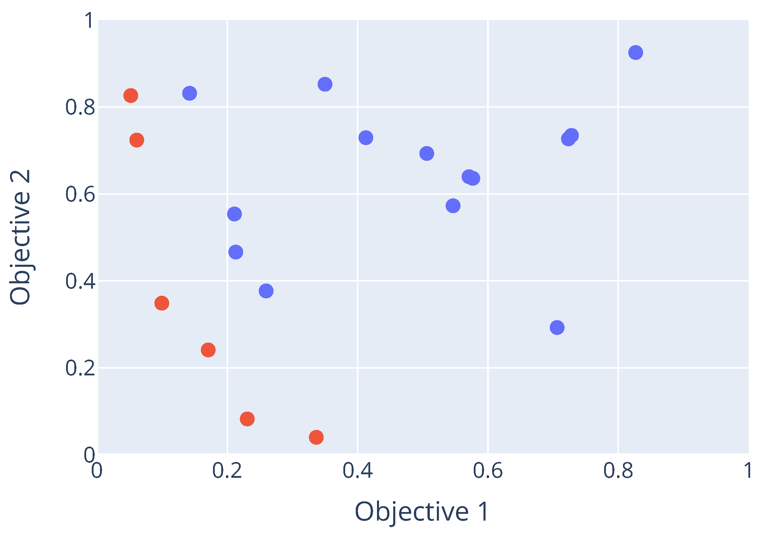
The definition of Pareto optimality, and by extension, the Pareto-optimal set, is based on the concept of non-dominance. Suppose two parameter configurations ${\theta }_1$ and ${\theta }_2$ with respective performance vectors $\mathbf{C}\left({\theta }_1\right)={\mathbf{C}}_1=\left[C_1^1,C_1^2,\dots ,C_1^n\right]$ and $\mathbf{C}\left({\theta }_2\right)={\mathbf{C}}_2=\left[C_2^1,C_2^2,\dots ,C_2^n\right]$. Configuration ${\theta }_1$ dominates configuration ${\theta }_2$ (denoted ${\theta }_1\prec {\theta }_2$), if and only if $C_1^i\le C_2^i\forall i\in \{1,2,\dots ,n\}$, and $\exists j\in \{1,2,\dots ,n\}$ such that $C_1^j<C_2^j$.

Now suppose a subset $\overline{\mathrm{\Theta }}\subset \mathrm{\Theta }$ where $\forall \overline{\theta }\in \overline{\mathrm{\Theta }}$, $\nexists \theta \in \mathrm{\Theta }\setminus \overline{\mathrm{\Theta }}$ such that $\theta \prec \overline{\theta }$. Such a set $\overline{\mathrm{\Theta }}$ contains non-dominated (or Pareto-optimal) parameter configurations. It is known as a Pareto-optimal set. The corresponding objective vectors of the configurations in this set, when plotted in objective space, will form a Pareto front. An example of a Pareto front is shown in Figure 1. Here, the red data points are the set of non-dominated points, while the blue dots are all points that are dominated by at least one point in the Pareto optimal set.

4.3. M-Race

This section describes the details of M-race, a multi-objective tuning algorithm for determining the Pareto-optimal set of parameter configurations. Based on F-race [6], M-race repeatedly evaluates control parameter configurations on a problem instance and eliminates suboptimal configurations as soon as enough statistical evidence is gathered to support worse performance. The main concern when generalising a single-objective tuning approach to a multi-objective setting is determining how a parameter configuration must be ranked in terms of performance when considering more than one objective. M-race employs non-dominated sorting, developed by Deb et al. [24], to rank configurations. By using this technique to assign a ranking, the same statistical test used by F-race to determine differences in rankings can be used to eliminate candidate configurations. Furthermore, the race is terminated when there is evidence that no more eliminations will take place. The rest of this section presents the details of M-race, with the pseudocode shown in Algorithm 2.

4.3.1. The Initial Sample

M-race begins by randomly sampling parameter configurations from the search space. Since this initial sample is the only set of configurations that will be evaluated, it is important that the sample covers as much of the search space as uniformly as possible. Sobol sequences, first introduced by Sobol’ [25], are a method developed for randomly generating points in a hypercube such that the points are distributed uniformly within the hypercube. The technique can be used when uniform sampling is required, and Klazar and Engelbrecht [8] showed that when used for sampling of control parameters, it provides good coverage of the parameter space, which allows for thorough exploration of the parameter space.

M-race employs Sobol sequences when performing the initial sample of parameter configurations. Due to the nature of the sequence generation, the length of the sequence can only be a power of two. Thus, the size of the initial sample is bound by this condition.

4.3.2. Determining Non-Dominated Configurations

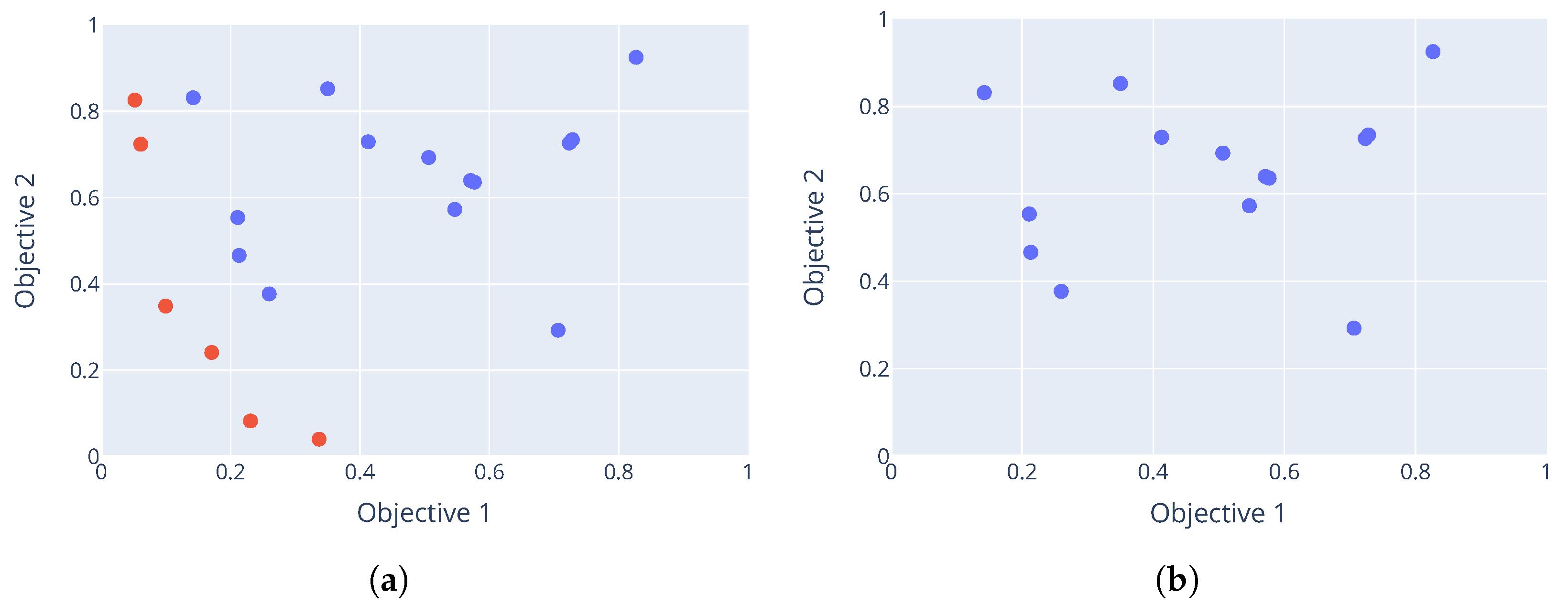
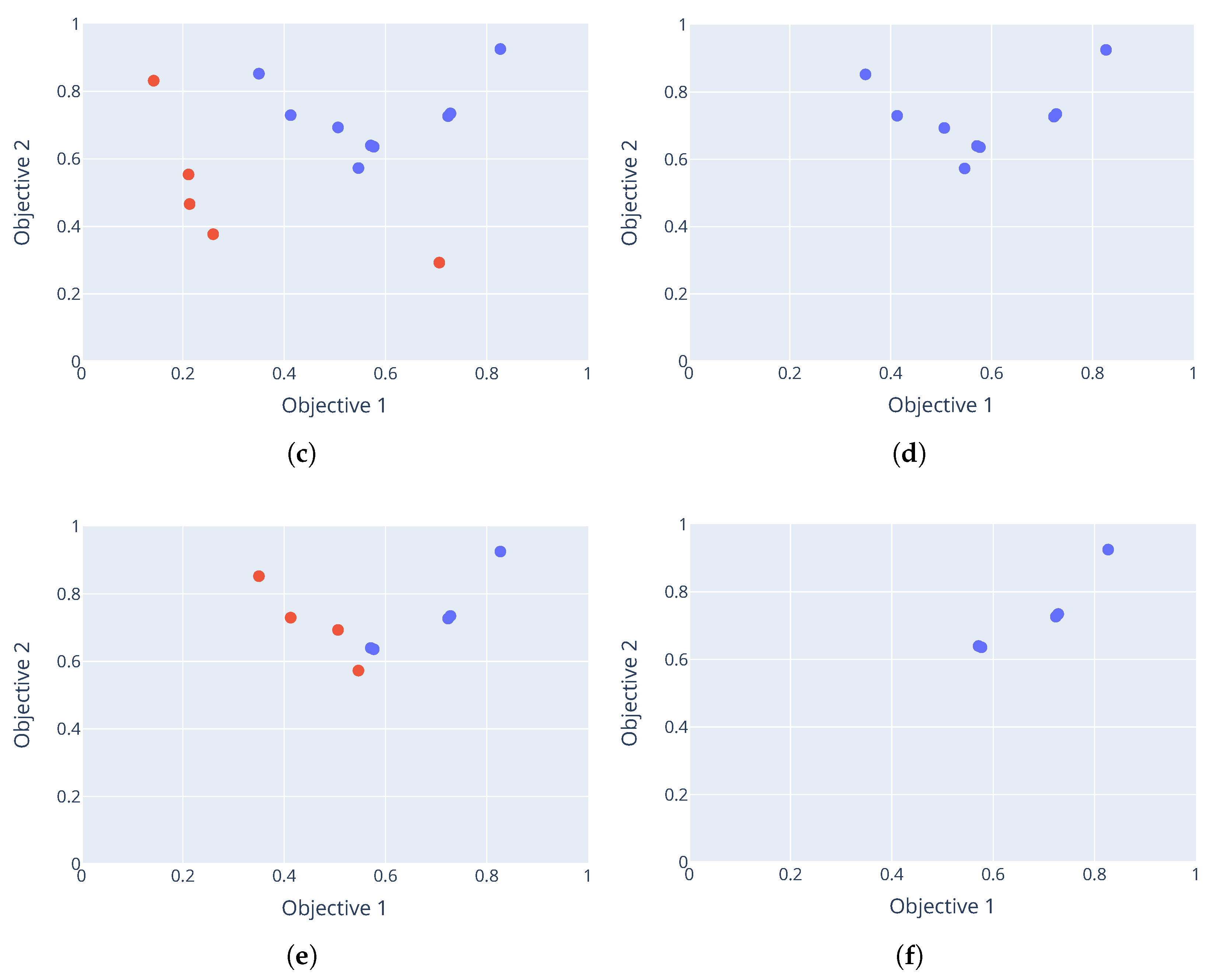
Non-dominated sorting was introduced by Deb et al. [24] for use in a multi-objective evolutionary algorithm. It is a technique for ranking points based on the ‘level’ of dominance. This ranking is used to eliminate underperforming candidates that consistently have a low rank.

Algorithm 2 M-race.

Sample N configurations uniformly with d control parameters each using a Sobol sequence. Let $\alpha$ be the chosen significance level.   $k\leftarrow 0$   Let ${\mathrm{\Theta }}_k$ be the surviving configs at iteration k   Let P be the history of p-values   while  $|{\mathrm{\Theta }}_k|>n_{min}$  do       Evaluate the performance of each $\theta \in {\mathrm{\Theta }}_k$       Rank ${\mathrm{\Theta }}_k$ using NDS       Perform Friedman test on ${\mathrm{\Theta }}_k$       Let p be the p-value of the test       $P\leftarrow P\cup p$       if $p<\alpha$ then           Remove worst configs from ${\mathrm{\Theta }}_k$           $P\leftarrow \varnothing$       else           Perform least-squares regression on P           Let m be the gradient of regression line           if $m\ge 0$ then return ${\mathrm{\Theta }}_k$           end if       end if       $k\leftarrow k+1$   end while   return  ${\mathrm{\Theta }}_0$

Suppose a set of parameter configurations ${\mathrm{\Theta }}_1$, with each configuration ${\theta }_i\in {\mathrm{\Theta }}_1$ having a corresponding performance vector ${\mathbf{C}}_i$. Ranking of the configurations proceed by determining the Pareto-optimal front of the performance vectors. All the parameter configurations that have corresponding performance vectors in this front are assigned the best rank of 1. Let this set of Pareto-optimal configurations be ${\overline{\mathrm{\Theta }}}_1\subset {\mathrm{\Theta }}_1$. Then, all configurations in ${\overline{\mathrm{\Theta }}}_1$ are removed from ${\mathrm{\Theta }}_1$ to form ${\mathrm{\Theta }}_2={\mathrm{\Theta }}_1\setminus {\overline{\mathrm{\Theta }}}_1$. This new set contains all the configurations that were dominated by those in the Pareto-optimal front. Now, the Pareto-optimal front of ${\mathrm{\Theta }}_2$ is calculated. Configurations in this front form another Pareto-optimal set ${\overline{\mathrm{\Theta }}}_2$ and are assigned a rank of 2. Again these configurations are removed to form ${\mathrm{\Theta }}_3={\mathrm{\Theta }}_2\setminus {\overline{\mathrm{\Theta }}}_2$. This process is repeated until all configurations have been assigned a rank. Figure 2 shows an example of non-dominated sorting. The red dots indicate the non-dominated solutions that form the Pareto front, while the blue dots represent dominated solutions that are assigned higher ranks in subsequent iterations of the sorting process.

4.3.3. Eliminating Candidates

Due to the stochastic nature of the performance of the parameter configurations, repeated evaluations and rankings are performed to gather evidence of performance. With several samples of ranks, the Friedman test described in Section 2.2 is employed to eliminate any candidates that show statistically significantly lower rankings than the rest. If there is not enough evidence to support the elimination of candidates, more evaluation and ranking are performed to gather additional evidence.

4.3.4. Stopping the Race

In F-race, the evaluation and elimination of candidates continue until only one or some specified number of candidates remains. This is no longer a valid stopping criterion for M-race, since the number of Pareto-optimal configurations is unknown. Section 2.2 also describes a way to prematurely stop the race if there is evidence that no further eliminations will occur. While this technique, introduced by Klazar and Engelbrecht [8], is merely an enhancement of F-race, it is a necessity as a termination condition for M-race.

It involves performing a regression analysis on the p-values of the Friedman test. The p-value indicates the probability of observing the rankings in the samples, assuming that all parameter configurations have an equal probability distribution of ranks (the null hypothesis). Initially, with few samples used in the test, the p-value would be high, since there is not enough evidence to warrant a rejection of the null hypothesis. As more evidence is gathered, this p-value decreases leading to an eventual rejection of the null hypothesis and the elimination of candidates. However, if all remaining candidates have equal distributions of ranks, the p-value will stagnate. If this happens, it is safe to conclude that it is unnecessary to gather more evidence, because it will not lead to further eliminations and the current set of remaining candidates can be considered Pareto-optimal. To detect this stagnation, a linear regression model is fitted to the p-values of the test. If the gradient of the regression line becomes greater than or equal to 0, the p-values have stagnated.

In addition to this stopping criterion, M-race also has a threshold to stop the race. If the number of remaining candidates falls below this threshold, the race is stopped. This is to prevent too few configurations from being found by the algorithm. It is also useful in controlling the running time of the algorithm. A larger threshold will stop the algorithm sooner. Algorithm 2 describes the M-race algorithm.

4.4. Empirical Procedure

This section details the empirical procedure followed in evaluating M-race. M-race was evaluated on a PSO [19] as well as a DE algorithm [26]. The test functions that were used as problems were as follows:

• Rastrigin [22]:

  $$f\left(\mathbf{y}\right)=10D+\sum _{i=0}^{D-1}\left(y_i^2-10cos\left(2\pi y_i\right)\right)$$
• Rana [27]:

  $$\begin{array}{cc}\hfill f\left(\mathbf{y}\right)& =\sum _{i=0}^{D-2}\left[y_i·cosa(y_{i+1},y_i)·sinb(y_{i+1},y_i)\right.\hfill \\ \hfill & +\left.\left(1+y_{i+1}\right)·sina(y_{i+1},y_i)·cosb\left(y_{i+1,y_i}\right)\right]\hfill \end{array}$$

  where

  $$\begin{array}{cc}\hfill a(y_{i+1},y_i)& =\sqrt{|y_{i+1}+y_i+1|}\hfill \\ \hfill b(y_{i+1},y_i)& =\sqrt{|y_{i+1}-y_i+1|}\hfill \end{array}$$
• Schwefel [28]:

  $$f\left(\mathbf{y}\right)=418.9829·D\sum _{i=0}^{D-1}{y}_{i}sin\sqrt{|y_i|}$$

Each function was tested in $D=20$ dimensions. The search space was a hypercube, centred on the origin, with lower and upper bounds defined in

Table 6. Lower and upper bounds of the hypercubes defining the search spaces.

Function	Lower Bound	Upper Bound
Rastrigin	−5.12	5.12
Rana	−512	512
Schwefel	−500	500

. A significance level of $\alpha =0.05$ was used for the Friedman test. An initial sample of 2048 parameter configurations were considered. Tuning was performed based on two performance objectives, namely accuracy and efficiency (see Section 3.2 for definitions), and a threshold value of $n_{min}=10$ was used.

Additionally, an analysis of the sensitivity to the initial sample was performed by running M-race on all the benchmark functions 10 times. The hypervolume measure [29] was used to compare the quality of the calculated Pareto fronts over the different tuning runs, for different initial sampling sizes of $2^k$, where k ranged from [5,10]. The calculated front is taken as the average of the performance of each parameter configuration with respect to each objective over the course of the tuning run. Since M-race has a minimum threshold where the algorithm is stopped prematurely, some configurations that remain may be dominated configurations. For the sake of this analysis, all such dominated configurations are removed before the hypervolume of the front is calculated. Furthermore, to compare the performance of M-race across different benchmark functions, the objective space is scaled to the interval [0,1] for each objective. This is performed using min–max normalisation. The reference point for the hypervolume measure is taken as (0,0). Thus, the smaller the hypervolume measure, the better the quality of the Pareto front. A PSO was tuned for the sake of the sensitivity analysis. In addition to the functions used for the general evaluation, sensitivity analysis was also conducted on the Ackley function defined in Section 3.2.

4.4.1. Particle Swarm Optimiser

The following parameters were tuned for the PSO:

• w, the inertia weight;
• $c_1$, the cognitive component;
• $c_2$, the social component;
• N, the number of particles in the swarm;

Parameters were sampled in the ranges $w\in [0,1]$, $c_1\in [0,2]$, $c_2\in [0,2]$, and $N\in [5,30]\cap \mathbb{Z}$.

4.4.2. Differential Evolution

The differential evolution algorithm has five total parameters to tune:

• N: The population size.
• Strategy: The evolutionary strategy to use. See [30] for a description.
• F: The mutation constant.
• $CR$: The crossover constant.
• T: The relative tolerance.
• A: The absolute tolerance.

Parameters were sampled in the ranges $N\in [5,30]\cap \mathbb{Z}$, $F\in [0,2]$, $CR\in [0,1]$, $T\in [0,1]$, $A\in [0,1]$. The strategy parameter is a categorical parameter and can take on the values DE/best/1/bin, DE/best/1/exp, DE/rand/1/exp, DE/randtobest/1/exp, DE/currenttobest/1/exp, DE/best/2/exp, DE/rand/2/exp, DE/randtobest/1/bin, DE/currenttobest/1/bin, DE/best/2/bin, DE/rand/2/bin, DE/rand/1/bin. Each categorical value was encoded as an integer so that it could be sampled by the Sobol sequence.

4.5. Results

This section presents and discusses the results obtained by the M-race algorithm.

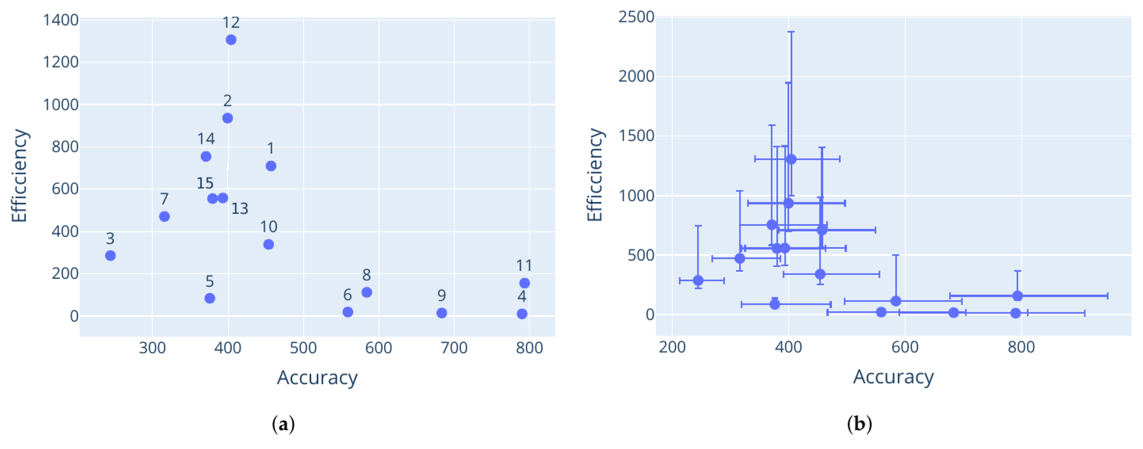
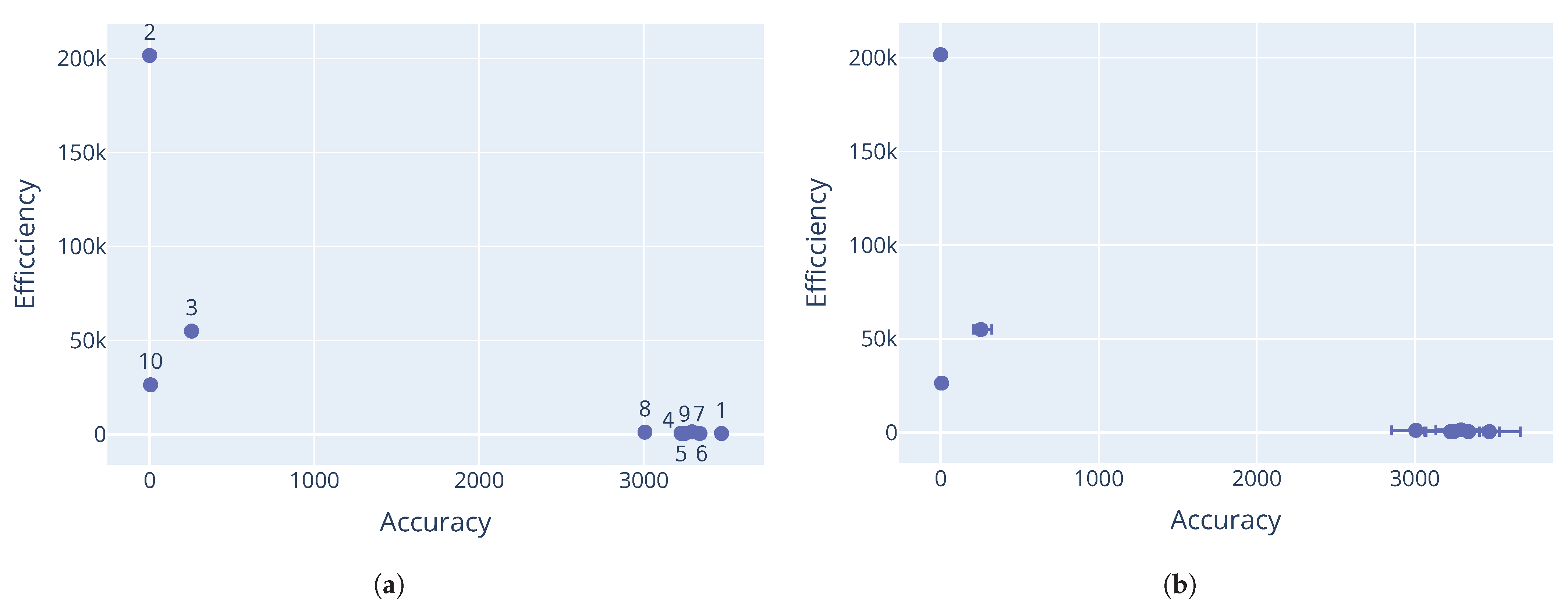
The Pareto-optimal parameter configurations that were found by M-race for the particle swarm optimiser are provided in

Table 7. PSO non-dominated parameter configurations for the Rastrigin function.

Label	w	${\mathit{c}}_1$	${\mathit{c}}_2$	N
1	0.0148	1.6057	0.7687	17
2	0.4764	1.6315	1.6076	23
3	0.231	1.8541	1.4445	12
4	0.7594	0.497	0.5405	9
5	0.0647	1.2039	1.3902	19
6	0.3799	0.6592	1.1041	10
7	0.9249	1.0682	0.7064	23
8	0.5435	1.6347	1.274	12
9	0.6338	1.558	1.5178	21
10	0.8139	1.9296	0.2609	22

,

Table 8. PSO non-dominated parameter configurations for the Rana function.

Label	w	${\mathit{c}}_1$	${\mathit{c}}_2$	N
1	0.0852	1.9385	0.6522	5
2	0.0345	0.568	1.0747	15
3	0.2756	1.5969	0.037	19
4	0.4022	0.4069	0.9894	21
5	0.7864	1.003	0.0141	9
6	0.4185	0.7537	1.1715	9
7	0.3894	1.4816	0.2774	29
8	0.6875	0.2586	0.5046	8
9	0.4948	0.1032	1.9488	19
10	0.1912	1.0772	0.9084	15
11	0.5677	1.2136	0.336	24
12	0.1698	0.5187	0.4446	27
13	0.2709	0.4904	1.6231	8
14	0.0431	1.4537	0.5232	26
15	0.0636	0.2606	1.3408	18

and

Table 9. PSO non-dominated parameter configurations for the Schwefel function.

Label	w	${\mathit{c}}_1$	${\mathit{c}}_2$	N
1	0.126	1.9799	1.992	15
2	0.9234	0.3485	1.0633	22
3	0.8687	0.7007	1.0449	15
4	0.6749	0.3639	0.8626	27
5	0.8472	1.3102	0.6326	11
6	0.6469	1.9117	1.9677	21
7	0.7004	1.8728	0.7175	28
8	0.8526	0.5382	1.704	26
9	0.8765	1.6726	0.4142	24

. The corresponding performance vectors are shown in Figure 3, Figure 4 and Figure 5. The performance data plotted here are the means of the performance for each configuration with respect to each objective. It is clear that different control parameter values result in different performance vectors, further supporting the claims made in Section 3. The results for each problem show a good Pareto-optimal front, indicating successful elimination of dominated configurations from the candidate set.

The minimum threshold was reached for the Rastrigin and Schwefel functions, which triggered an early stop. This explains why configuration 10 for the Rastrigin function and configuration 9 for the Schwefel function seem to dominate the other configurations. Further evaluations would likely have eliminated more configurations, leaving only these dominant solutions in the Pareto front.

Having dominated solutions remaining in the resulting Pareto-optimal set is evidence of a weakness with the M-race algorithm. Like F-race, only the initial sample of parameter configurations are considered in the race. It is possible that only a small number of configurations from the initial sample are truly non-dominant. If the initial sample was even larger, more non-dominated configurations could have been discovered. This shows that the performance of M-race is sensitive to the initial configuration sample.

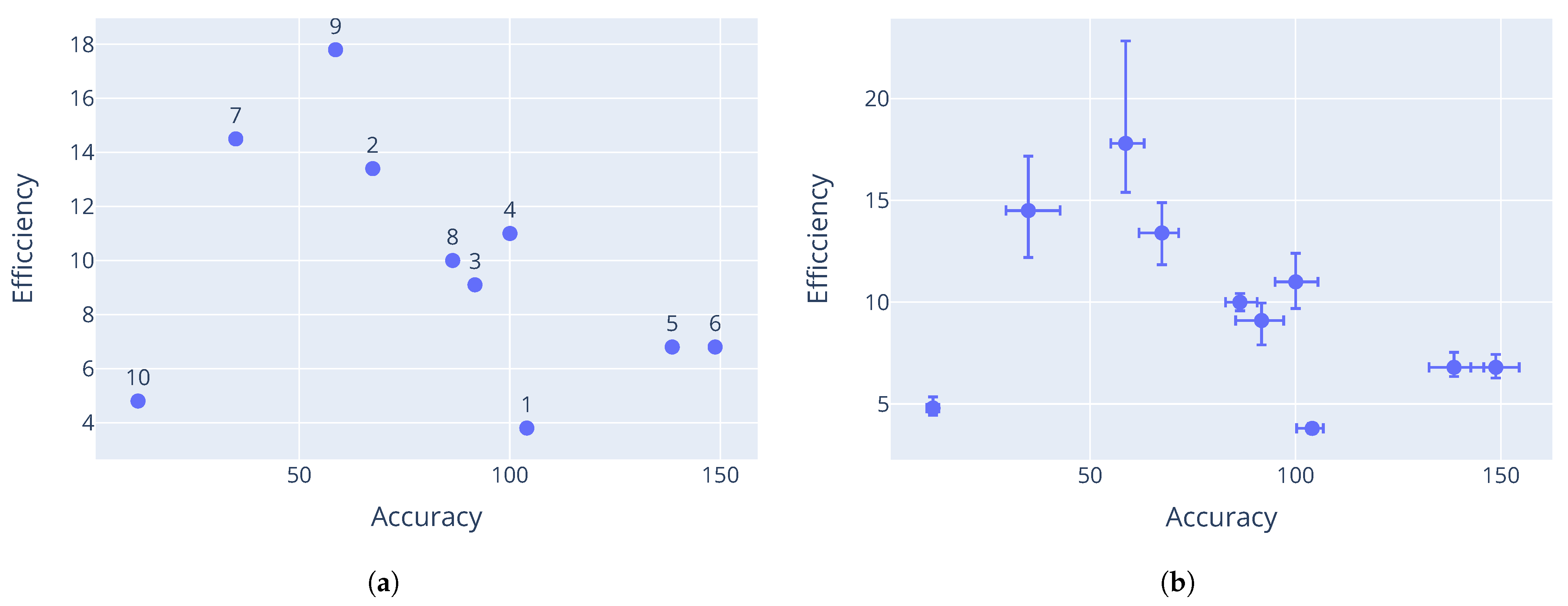
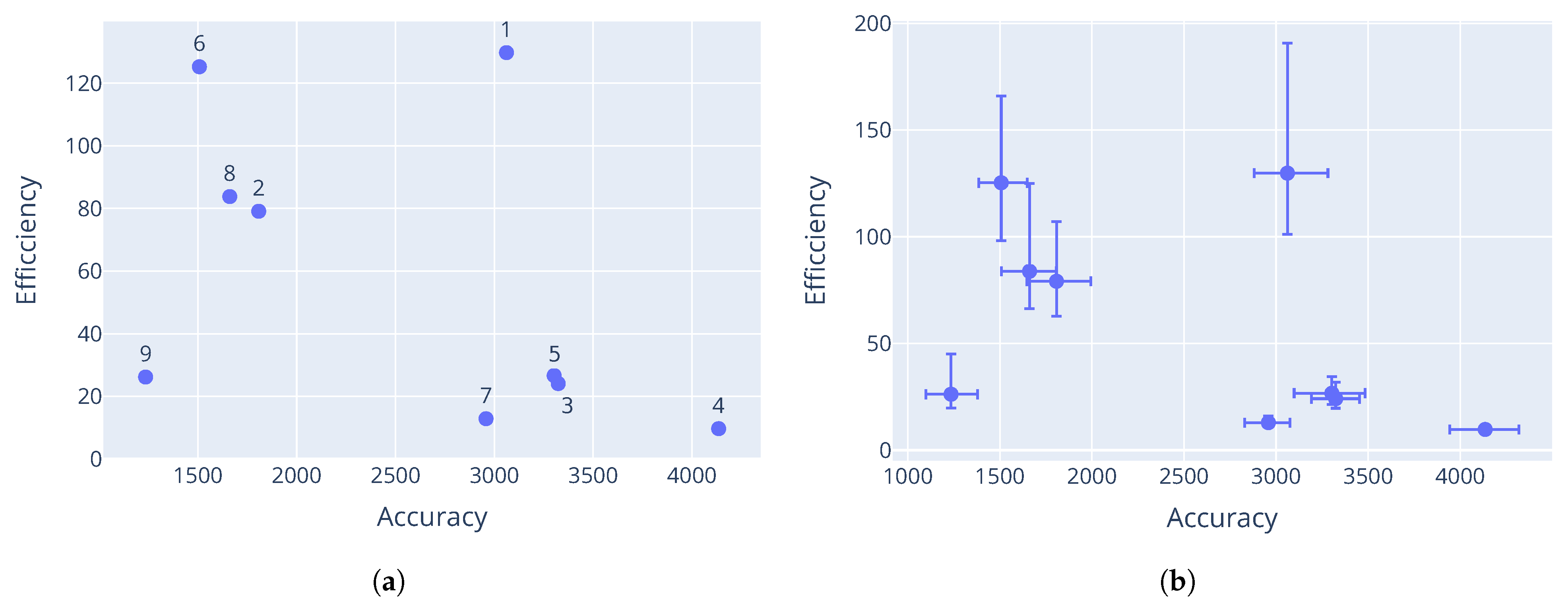
The Rana function also shows a few configurations that appear to dominate the rest. However, as can be seen in Figure 4b, the performance of the configurations has significant variance. The minimum threshold was not triggered on this function. Thus, despite the mean performance of the configurations, there is no statistical evidence (at a significance level of 0.05) that the presented configurations dominate each other.

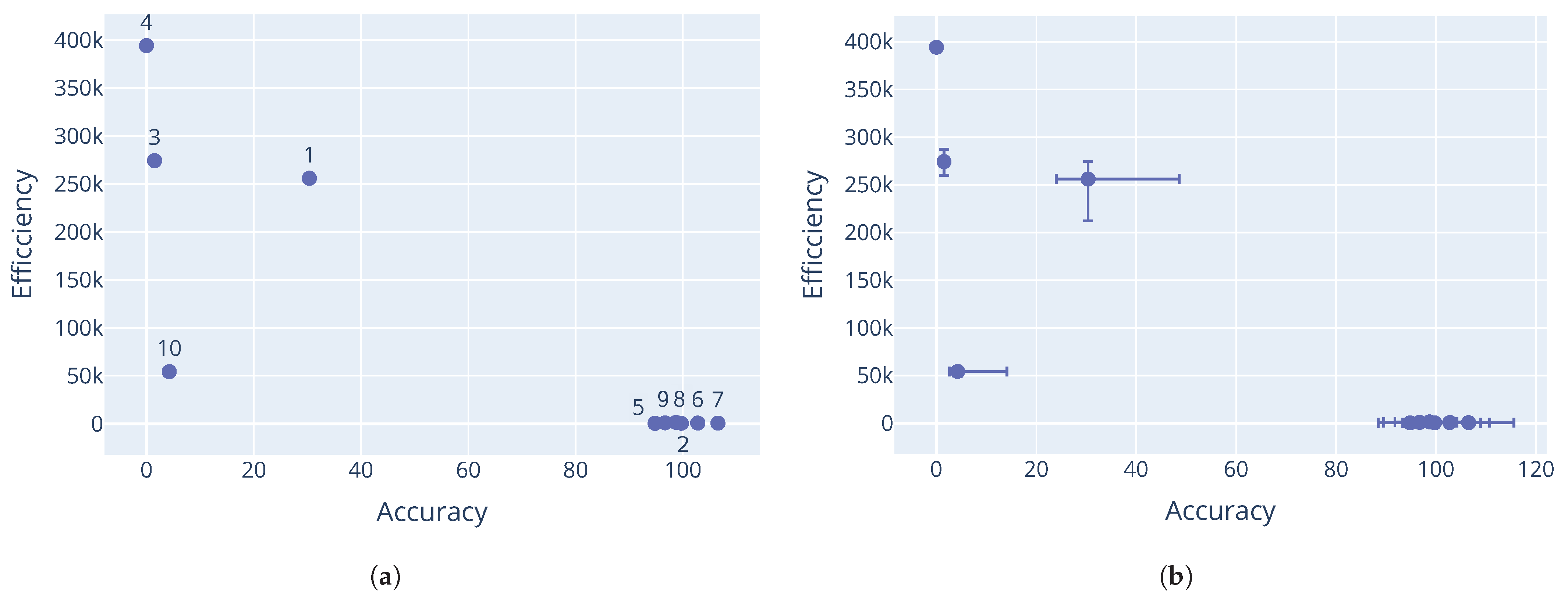
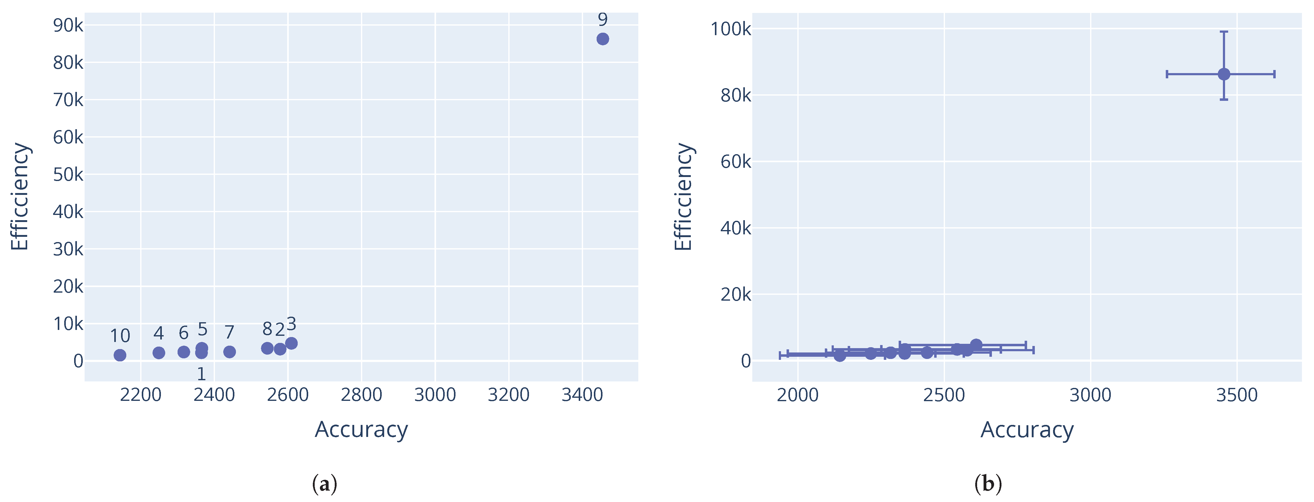
Looking at the differential evolution results on the Rastrigin and Schwefel function in Figure 6, decent non-dominated solutions were discovered, albeit with a rather large gap in the Pareto-optimal front, indicating that better coverage of the search space was needed. Results from the Rana function in Figure 7 further illustrate the sensitivity to the initial sample. Here the minimum threshold was triggered, but it is clear that more candidates would have been eliminated had the race continued. This would have resulted in only one dominant candidate being discovered. Similar results were observed for the Schwefel function in Figure 8. Corresponding parameter values for the differential evolution algorithm are shown in

Table 10. DE control parameter configurations for the Rastrigin function.

Label	N	Strategy	F	$\mathbf{CR}$	T	A
1	5	DE/currenttobest/1/exp	1.9559	0.0935	0.1122	0.3195
2	7	DE/rand/2/bin	0.0624	0.2985	0.6217	0.4909
3	14	DE/randtobest/1/bin	0.4642	0.4946	0.0887	0.8393
4	14	DE/rand/1/exp	1.2777	0.5097	0.077	0.4769
5	5	DE/rand/2/bin	1.1005	0.393	0.9706	0.393
6	13	DE/currenttobest/1/exp	0.9232	0.4025	0.6186	0.8046
7	10	DE/rand/1/bin	0.878	0.4909	0.7785	0.1921
8	29	DE/randtobest/1/exp	0.701	0.4483	0.3664	0.2892
9	18	DE/rand/2/exp	1.3405	0.9267	0.3994	0.9853
10	9	DE/randtobest/1/bin	0.2343	0.2757	0.1096	0.6826

,

Table 11. DE control parameter configurations for the Rana function.

Label	N	Strategy	F	$\mathbf{CR}$	T	A
1	10	DE/best/1/bin	0.8621	0.678	0.8867	0.773
2	20	DE/currenttobest/1/bin	1.7235	0.7477	0.6799	0.2787
3	29	DE/rand/1/bin	0.325	0.0961	0.9689	0.4053
4	11	DE/best/1/bin	1.6361	0.9089	0.7503	0.4309
5	9	DE/rand/2/bin	0.0437	0.7525	0.3221	0.8904
6	7	DE/randtobest/1/exp	0.6712	0.95	0.4842	0.7173
7	5	DE/randtobest/1/exp	1.364	0.5665	0.9832	0.4935
8	26	DE/randtobest/1/bin	1.1143	0.697	0.7702	0.3755
9	6	DE/rand/2/bin	1.8174	0.5336	0.1084	0.4341
10	5	DE/rand/1/bin	0.4412	0.7342	0.91	0.2763

and

Table 12. DE control parameter configurations for the Schwefel function.

Label	N	Strategy	F	$\mathbf{CR}$	T	A
1	5	DE/best/2/bin	0.3573	0.0111	0.169	0.9515
2	19	DE/rand/1/bin	0.8913	0.1194	0.057	0.257
3	17	DE/best/1/exp	0.2677	0.7468	0.0853	0.6672
4	6	DE/best/1/bin	0.2278	0.1407	0.3483	0.4018
5	5	DE/currenttobest/1/exp	1.2763	0.9164	0.4119	0.6636
6	5	DE/rand/1/bin	0.7773	0.2686	0.9745	0.3436
7	29	DE/rand/1/exp	0.2575	0.4623	0.398	0.3932
8	DE/randtobest/1/exp	23	0.8027	0.8998	0.4279	0.2945
9	5	DE/best/1/exp	0.117	0.7154	0.8709	0.7443
10	21	DE/randtobest/1/bin	0.0029	0.7324	0.0349	0.0934

.

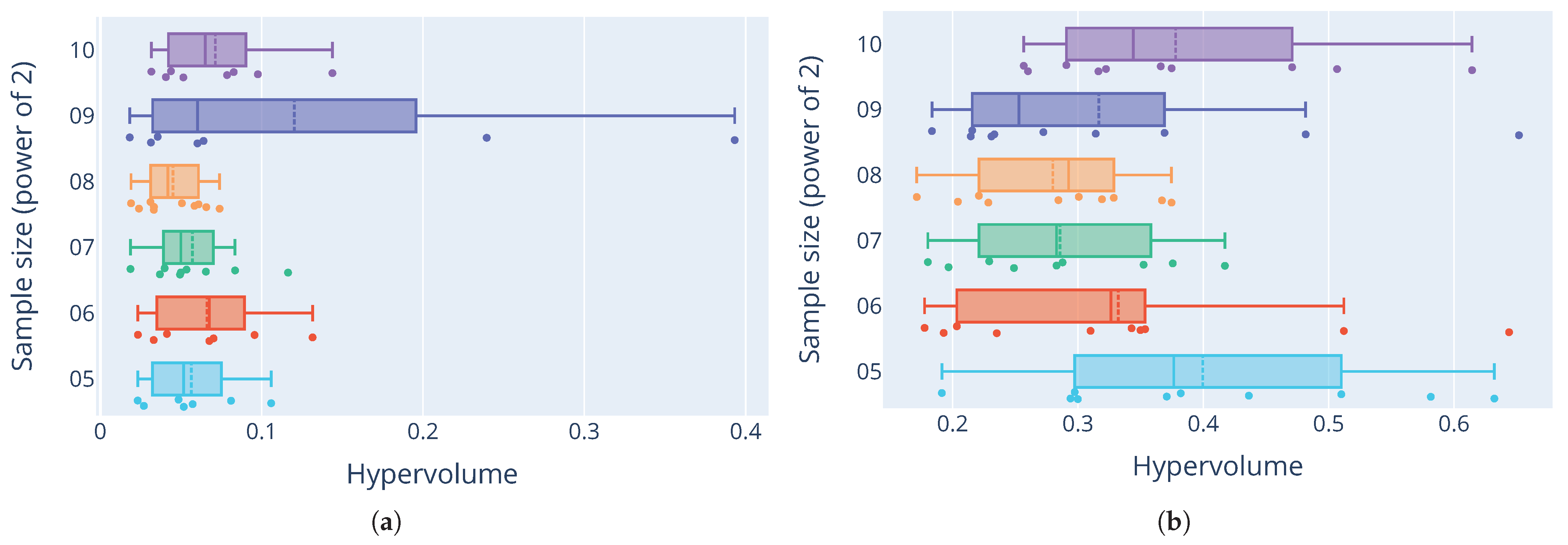
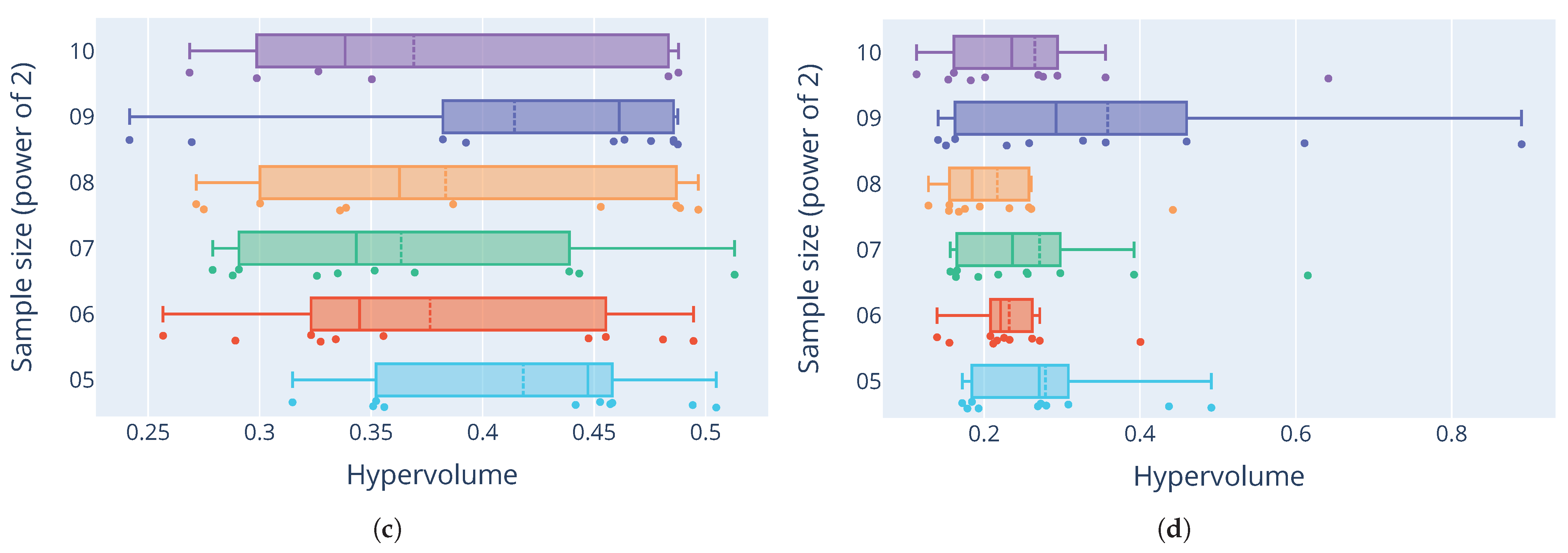
The results of the sensitivity analysis generally show varying levels of the quality of the generated Pareto-optimal fronts. For the Ackley function, Figure 9a shows consistently low hypervolumes for most sample sizes, apart from a sample size of $2^9$, which shows unusually high outliers. For the Rastrigin function in Figure 9b, the distribution of hypervolumes is more varied when comparing different sample sizes. The distributions tend to be skewed towards smaller hypervolume measures. Still, large variance of the hypervolumes indicates high sensitivity to the initial distribution of the starting sample. The Rana function in Figure 9c has a much larger variance in the quality of the fronts. The stark difference between distributions for this function and the others show how the quality of the tuned configurations differs not only between different sizes of the initial sample, but the underlying optimisation problem itself. Some problems prove to be much more difficult to tune consistently. Figure 9d shows that parameter configurations for the Schwefel function had similar quality distributions as those for the Ackley function. Hypervolumes are on average relatively small, with some outliers, especially with a sample size of $2^9$. As these results show, M-race is very sensitive to the quality and size of the initial sample of parameters.

5. Conclusions

This study investigated the relationship between the tuned values of meta-heuristic control parameters and the performance objective that is used for the tuning process. Using iterated F-race, it was shown that different values for control parameters are optimal for different performance objectives.

Multi-objective tuning allows for multiple performance objectives to be taken into account when tuning a meta-heuristic. However, with multiple objectives being considered, a single parameter configuration can no longer be considered optimal. Some configurations result in better performance for one objective than another. Multi-objective tuning thus requires the discovery of several Pareto-optimal parameter configurations, each representing different levels of trade-off between competing performance objectives.

This paper presented M-race, a multi-objective tuning algorithm that discovers Pareto-optimal control parameters using a racing strategy. It uses non-dominated sorting to rank candidate parameter configurations based on their performance on each objective. Results showed that M-race has the ability to discover Pareto-optimal configurations for both a particle swarm optimiser and a differential evolution algorithm on different benchmark optimisation problems. However, the quality of the generated Pareto-optimal fronts is sensitive to the initial sample of candidate configurations. Good coverage of the search space with many candidate configurations is required for decent results.

Future work should address this sensitivity through improved sampling strategies. A promising direction is the development of an iterative version similar to iterated F-race, where new samples are drawn from an already discovered Pareto-optimal set to further explore the search space. However, the feasibility of such an approach requires careful consideration given the sensitivity of meta-heuristics to parameter variations. Additionally, investigating adaptive sampling methods that adjust coverage based on the emerging Pareto front could enhance the robustness of the tuning process. Future research could also evaluate M-race on other meta-heuristic algorithms beyond PSO and DE to further validate its generalisability across different algorithmic paradigms.

References

- Dymond, A.; Engelbrecht, A.; Kok, S.; Heyns, P. Tuning Optimization Algorithms Under Multiple Objective Function Evaluation Budgets. IEEE Trans. Evol. Comput. 2015, 19, 341–358. [Google Scholar] [CrossRef]
- Ugolotti, R.; Cagnoni, S. Analysis of evolutionary algorithms using multi-objective parameter tuning. In Proceedings of the Annual Conference on Genetic and Evolutionary Computation, Vancouver, BC, Canada, 12–16 July 2014; pp. 1343–1350. [Google Scholar]
- Zhang, T.; Georgiopoulos, M.; Anagnostopoulos, G. S-Race: A multi-objective racing algorithm. In Proceedings of the 15th Annual Conference on Genetic and Evolutionary Computation, Amsterdam, The Netherlands, 6–10 July 2013; pp. 1565–1572. [Google Scholar]
- Ridge, E. Design of Experiments for the Tuning of Optimisation Algorithms; University of York: York, UK, 2007. [Google Scholar]
- Montgomery, D. Design and Analysis of Experiments; John Wiley & Sons: Hoboken, NJ, USA, 2020. [Google Scholar]
- Birattari, M.; Yuan, Z.; Balaprakash, P.; Stützle, T. F-Race and Iterated F-Race: An Overview. In Experimental Methods for the Analysis of Optimization Algorithms; Springer: Berlin/Heidelberg, Germany, 2010; pp. 311–336. [Google Scholar] [CrossRef]
- Conover, W. Practical Nonparametric Statistics; John Wiley & Sons: Hoboken, NJ, USA, 1999; pp. 369–371. [Google Scholar]
- Klazar, R.; Engelbrecht, A. Parameter optimization by means of statistical quality guides in F-Race. In Proceedings of the IEEE Congress on Evolutionary Computation, Beijing, China, 6–11 July 2014; pp. 2547–2552. [Google Scholar]
- Bartz-Beielstein, T.; Lasarczyk, C.; Preuß, M. Sequential parameter optimization. In Proceedings of the IEEE Congress on Evolutionary Computation, Edinburgh, UK, 2–5 September 2005; Volume 1, pp. 773–780. [Google Scholar]
- Nannen, V.; Eiben, A. Efficient relevance estimation and value calibration of evolutionary algorithm parameters. In Proceedings of the IEEE Congress on Evolutionary Computation, Singapore, 25–28 September 2007; pp. 103–110. [Google Scholar]
- Mockus, J. The Bayesian Approach to Local Optimization. In Bayesian Approach to Global Optimization: Theory and Applications; Springer: Dordrecht, The Netherlands, 1989; pp. 125–156. [Google Scholar] [CrossRef]
- Brochu, E.; Cora, V.M.; de Freitas, N. A Tutorial on Bayesian Optimization of Expensive Cost Functions, with Application to Active User Modeling and Hierarchical Reinforcement Learning. Technical Report UBC TR-2009-023; Department of Computer Science, University of British Columbia: Vancouver, BC, Canada, 2009. [Google Scholar]
- Roman, I.; Ceberio, J.; Mendiburu, A.; Lozano, J. Bayesian optimization for parameter tuning in evolutionary algorithms. In Proceedings of the IEEE Congress on Evolutionary Computation, Vancouver, BC, Canada, 24–29 July 2016; pp. 4839–4845. [Google Scholar] [CrossRef]
- Bergstra, J.; Bardenet, R.; Bengio, Y.; Kégl, B. Algorithms for hyper-parameter optimization. Adv. Neural Inf. Process. Syst. 2011, 24, 2546–2554. [Google Scholar]
- Li, L.; Jamieson, K.; DeSalvo, G.; Rostamizadeh, A.; Talwalkar, A. Hyperband: A novel bandit-based approach to hyperparameter optimization. J. Mach. Learn. Res. 2018, 18, 1–52. [Google Scholar]
- Holm, S. A Simple Sequentially Rejective Multiple Test Procedure. Scand. J. Stat. 1979, 6, 65–70. [Google Scholar]
- Zhang, T.; Georgiopoulos, M.; Anagnostopoulos, G.C. SPRINT Multi-Objective Model Racing. In Proceedings of the Annual Conference on Genetic and Evolutionary Computation, Madrid, Spain, 11–15 July 2015; pp. 1383–1390. [Google Scholar] [CrossRef]
- Wald, A. Sequential Analysis; Courier Corporation: North Chelmsford, MA, USA, 2004. [Google Scholar]
- Eberhart, R.; Kennedy, J. A new optimizer using particle swarm theory. In Proceedings of the Sixth International Symposium on Micro Machine and Human Science, Nagoya, Japan, 4–6 October 1995; pp. 39–43. [Google Scholar] [CrossRef]
- Shi, Y.; Eberhart, R. A modified particle swarm optimizer. In Proceedings of the IEEE International Conference on Evolutionary Computation, Anchorage, AK, USA, 4–9 May 1998; pp. 69–73. [Google Scholar] [CrossRef]
- Poli, R. Mean and Variance of the Sampling Distribution of Particle Swarm Optimizers During Stagnation. IEEE Trans. Evol. Comput. 2009, 13, 712–721. [Google Scholar] [CrossRef]
- Hoffmeister, F.; Bäck, Y. Genetic Algorithms and evolution strategies: Similarities and differences. In Parallel Problem Solving from Nature; Springer: Berlin/Heidelberg, Germany, 1991; pp. 455–469. [Google Scholar]
- Ackley, D. A Connectionist Machine for Genetic Hillclimbing; Kluwer Academic Publishers: Norwell, MA, USA, 1987; pp. 82–99. [Google Scholar]
- Deb, K.; Agrawal, S.; Pratap, A.; Meyarivan, T. A Fast Elitist Non-dominated Sorting Genetic Algorithm for Multi-objective Optimization: NSGA-II. In Parallel Problem Solving from Nature PPSN VI; Springer: Berlin/Heidelberg, Germany, 2000; pp. 849–858. [Google Scholar]
- Sobol’, I. On the distribution of points in a cube and the approximate evaluation of integrals. USSR Comput. Math. Math. Phys. 1967, 7, 86–112. [Google Scholar] [CrossRef]
- Storn, R.; Price, K. Differential Evolution—A Simple and Efficient Heuristic for global Optimization over Continuous Spaces. J. Glob. Optim. 1997, 11, 341–359. [Google Scholar] [CrossRef]
- Vanaret, C.; Gotteland, J.; Durand, N.; Alliot, J. Certified Global Minima for a Benchmark of Difficult Optimization Problems. arXiv 2020, arXiv:2003.09867. [Google Scholar]
- Schwefel, H. Numerical Optimization of Computer Models; John Wiley & Sons, Inc.: Hoboken, NJ, USA, 1981. [Google Scholar]
- Cao, Y.; Smucker, B.; Robinson, T. On using the hypervolume indicator to compare Pareto fronts: Applications to multi-criteria optimal experimental design. J. Stat. Plan. Inference 2015, 160, 60–74. [Google Scholar] [CrossRef]
- Mezura-Montes, E.; Velázquez-Reyes, J.; Coello Coello, C. A Comparative Study of Differential Evolution Variants for Global Optimization. In Proceedings of the 8th Annual Conference on Genetic and Evolutionary Computation, Seattle, WA, USA, 8–12 July 2006; pp. 485–492. [Google Scholar] [CrossRef]