Sampling Method Based on Fuzzy Membership for Computing Negative Sample Credibility and Its Applications

Abstract

Current sampling methods do not provide effective quantitative assessment mechanisms for evaluating the intrinsic credibility of negative samples. This impedes the systematic quantification of the effect of misselection of geologically predisposed areas (i.e., potential landslide zones) as negative samples on the accuracy of landslide susceptibility evaluation models. To overcome this challenge, this study proposes a fuzzy membership-based sampling method for assessing negative sample credibility in the Liangshan Yi Autonomous Prefecture, where credibility is defined as the confidence level of stable nonlandslide samples. Subsequently, negative samples were sampled across stratified credibility thresholds to construct a frequency ratio–random forest coupled model. The influence of negative sample credibility on model performance was then systematically evaluated using various metrics, including the F1-score (metrics for evaluating classification performance), area under the receiver operating characteristic curve (AUC), and actual landslide distribution ratio (landslide proportion) in high-susceptibility zones. The results are as follows: (1) Increasing the credibility threshold progressively improves model precision while inducing systematic overestimation bias in regional susceptibility assessment; (2) Integrated analysis of model performance and landslide distribution characteristics (where recall, F1-score, and AUC values initially increase then decrease) confirms the optimal effectiveness when selecting negative samples within a credibility threshold range of 0.7–1.0. This study innovatively achieves quantitative optimization of negative samples and provides a universal solution for improving the performance of diverse models reliant on negative sampling strategies.

1. Introduction

Landslide susceptibility mapping refers to the evaluation and prediction of the spatial likelihood of landslide occurrence in a region based on its disaster-predisposing geological conditions through qualitative analyses or quantitative modeling [1]. This assessment serves not only as a critical component of disaster prevention and mitigation but also as a fundamental basis for resource management, environmental protection, and policy formulation [2]. With technological advancements, machine learning (ML) models have emerged as vital tools for improving assessment accuracy because of their superior nonlinear mapping capabilities. However, their application efficacy is significantly constrained by training data quality, particularly the credibility of negative samples [3,4].

The credibility of negative samples, which represent confidence levels in stable nonlandslide instances, constrains the precision and accuracy of ML models [4]. However, no standardized criteria for selecting scientifically sound negative samples have been established. Based on method similarities, existing sampling approaches can be categorized into four distinct types. Four primary methodologies for negative sample selection have been established based on geographical similarities in sampling mechanisms: (1) random sampling, involving stochastic selection across the study area, ensures uniform spatial distribution devoid of subjective bias but risks contamination by latent landslide instances, i.e., spatial locations exhibiting predisposing conditions for slope failure without historical occurrences, thereby compromising interclass discriminability [5]; (2) buffer-controlled sampling selects samples beyond predefined perimeters around landslides, leveraging environmental dissimilarity while introducing subjectivity through arbitrary buffer distances and neglecting regional geomorphological homogeneity [6,7]; (3) model-coupled sampling derives negative samples from low-susceptibility zones predicted by negative-sample-independent models or via physical modeling-based slope safety factors, thereby achieving superior prediction accuracy though constrained by computational inefficiency at scale [8]; (4) environmental factor-constrained sampling employs single/multiple constraints (e.g., low-gradient zones, extrapolation sampling), offering high efficiency and generalizability but suffering from either overemphasis on specific factors (single-constraint) or stochastic noise introduction (multi-constraint) that degrades sample integrity [9]. Despite widespread adoption of the aforementioned negative sampling methodologies, two fundamental challenges persist [10]: (1) the absence of a robust quantitative metric for evaluating the credibility of selected nonlandslide samples and (2) inadequate investigation into the mechanistic effect of credibility thresholds on the accuracy of susceptibility evaluation models. Addressing these challenges is critical for fully exploiting the predictive capability and generalizability of ML approaches.

Given these considerations, this study selected the Liangshan Yi Autonomous Prefecture in Sichuan Province, China, which is a region characterized by the densest tectonic structures, most intense seismic activity, and highest geohazard susceptibility, as its research area [11]. This study focuses on the following two primary objectives. (1) To address the lack of quantitative evaluation criteria for negative samples, this study proposes a fuzzy membership-based sampling method to compute the credibility of negative samples (defined as the confidence level of stable nonlandslide instances). The proposed method quantifies the “dissimilarity” between candidate nonlandslide locations and known landslide environments based on fuzzy membership theory and generates spatially continuous credibility distribution maps (with a value range of 0–1), where higher scores indicate more reliable nonlandslide attributes. (2) To investigate the mechanistic influence of negative sample credibility thresholds on landslide susceptibility model accuracy, we rigorously evaluated the effects of varying credibility thresholds on model performance and landslide susceptibility zoning using various metrics, including F1-score, the area under the receiver operating characteristic curve (AUC), and landslide ratio. This analysis aims to decipher the mechanisms by which credibility thresholds govern model precision. This study aims to (1) propose a sampling method capable of quantitatively evaluating negative sample credibility to generate high-precision landslide susceptibility maps, thereby providing guidance for landslide risk management in the Liangshan Prefecture; (2) elucidate the quantitative relationship between negative sample credibility thresholds and model accuracy to identify the optimal selection threshold for negative samples in landslide susceptibility assessment in the Liangshan Prefecture; and (3) establish a transferable negative sample sampling framework to provide a practical paradigm for geohazard-prone regions facing similar challenges globally.

2. Study Areas and Data Sources

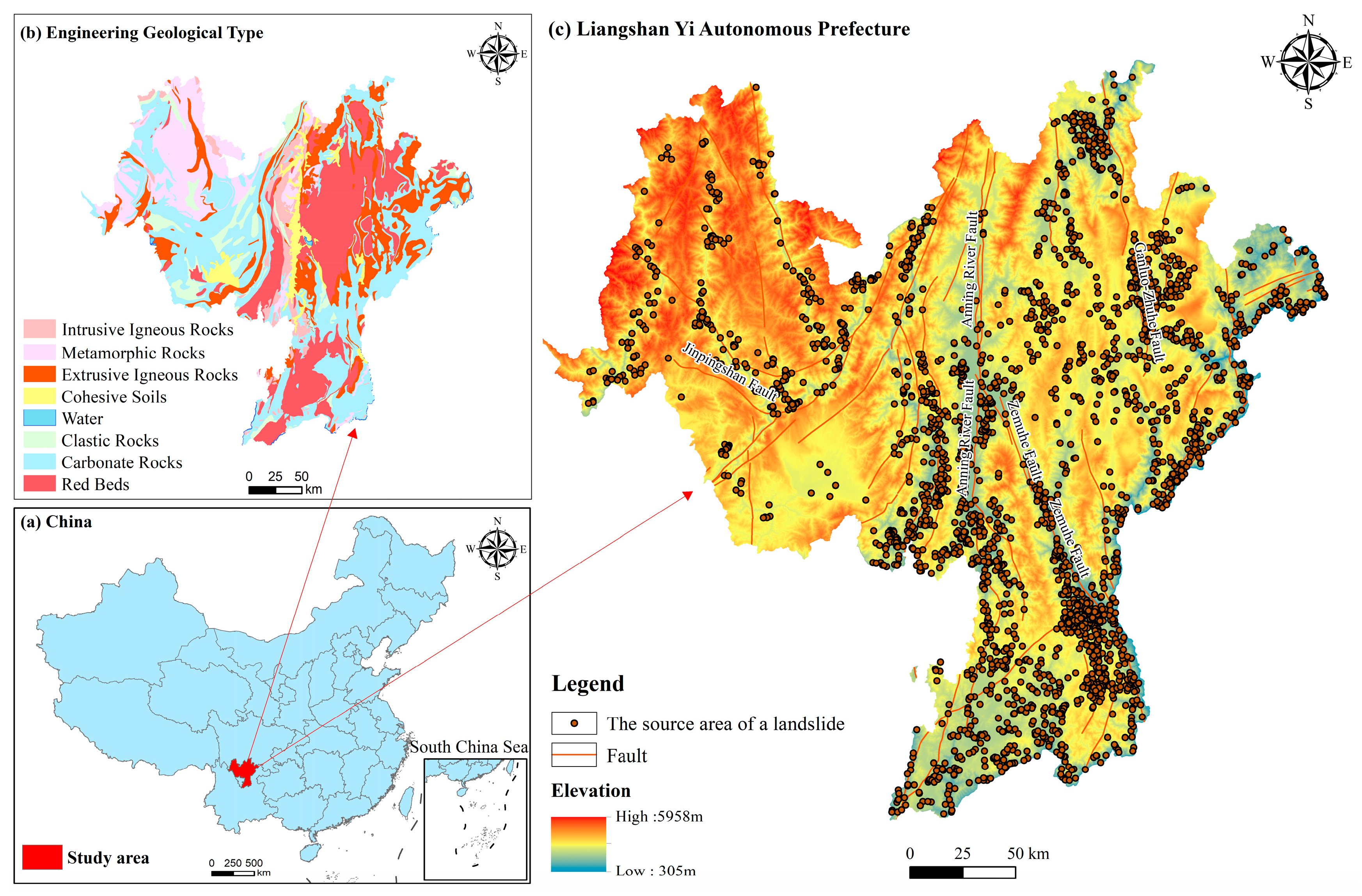
2.1. Study Areas

The Liangshan Yi Autonomous Prefecture is in southwestern Sichuan Province, China, where the western edge of the Yangtze Craton meets the eastern edge of the Tibetan Plateau. The Liangshan Prefecture is in the southern region of the Sichuan–Yunnan tectonic belt. The primary active fractures in the study area include the Anning River Fault, Zemuhe Fault, Ganluo–Zhuhe Fault, Xihe–Meigu Fault, Ebian–Jinyang Fault, and Jinpingshan Fault. The Anning River Fault is the most significant fracture in the Liangshan Prefecture.

The primary strata in the area include periods (P1, P2), which are predominantly composed of limestone and basalt. During the Triassic period (T1, T2, T3), the strata comprised interbedded sandstone and mudstone with interspersed tuff. During the Jurassic period (J1, J2, J3), the strata comprised mudstone and sandstone interbedded with tuff and conglomerate layers interbedded with sandstone. During the Cretaceous period (K1, K2), the strata comprised sandstone interbedded with marl and conglomerates. Based on the engineering geological properties, genesis types, and structural characteristics of the rocks, the study area is classified into seven engineering geology rock types: cohesive soils, clastic rocks, carbonate rocks, intrusive igneous rocks, extrusive igneous rocks, red beds, and metamorphic rocks. The distribution of these rocks is illustrated in Figure 1.

2.2. Data Sources

By the end of 2022, 2681 landslides had been reported in the Liangshan Prefecture. Statistical analysis indicated that earthy landslides were the most prevalent, with 2619 occurrences, accounting for 97.7% of the total. In contrast, rocky landslides are relatively rare, with only 62 occurrences, representing 2.3% of the cases. The landslide data and sources of the evaluation factors used in this study are presented in

Table 1. Multisource data and parameters for landslide assessment in the Liangshan Prefecture.

Name	Source	Data Type	Scale
Landslides	Chengdu Geological Survey Center	Shop
DEM	Global digital elevation model(GDEM)	Tiff	90 m
Geological information	National Geological Data Center	Shop	1:200,000
Roads	Digital Earth Science Platform	Shop	1:100,000
Rivers	Resource and Environmental Science Data Platform	Shop	1:100,000
Faults	National Earthquake Data Center	Shop	1:100,000

.

3. Methods

The workflow of this study is illustrated in Figure 2.

(1) Landslide Dataset Construction: this study first established a precise historical landslide distribution layer by georeferencing and spatially positioning the collected historical landslide inventory data for the research area using the ArcGIS platform. Subsequently, 14 evaluation factors were selected: (1) elevation, (2) slope, (3) aspect, (4) surface cutting depth (SCD), (5) plan curvature (PLC), (6) profile curvature (PRC), (7) engineering geological group (EGG), (8) soil erosion intensity (SEI), (9) soil thickness (STK), (10) soil moisture content (SMC), (11) population density (PD), (12) road density (RD), (13) fault density (FD), and (14) drainage density (DD). All raw factor data underwent standardized preprocessing in ArcGIS, including unified spatial reference conversion, projection adjustment, resampling (to a consistent resolution), and research area clipping. Topographic factors (elevation, slope, aspect, SCD, PLC, and PRC) were derived using Digital Elevation Model (DEM) surface analysis tools, and density-based factors (RD, FD, DD, and PD) were generated using the kernel density estimation method. Finally, a structured landslide susceptibility assessment database was constructed by spatially integrating the historical landslide distribution layer with the preprocessed raster data of the 14 evaluation factors.

(2) Quantification of Negative Sample Credibility and Construction of Negative Sample Sets: first, evaluation factors were screened based on their coefficient of variation, nonlinear correlation with landslides, and collinearity diagnosis, ultimately selecting elevation, SEI, and SMC. Using the fitting tools in Origin software, the functional relationships between the selected evaluation factors and landslide frequency (the relative number of landslides occurring within specific factor classes) were fitted to construct fuzzy membership functions. Weighted by the proportional contribution of the correlation of each factor (weight = factor correlation/sum of all factor correlations), a spatially continuous negative sample credibility distribution map was generated through comprehensive weighted calculations in ArcGIS version 10.8.2 using the Raster Calculator. Based on predefined credibility thresholds, five negative sample sets were constructed: Set A (credibility: 0.5–1.0), Set B (credibility: 0.6–1.0), Set C (credibility: 0.7–1.0), Set D (credibility: 0.8–1.0), and Set E (credibility: 0.9–1.0).

(3) Construction of the Frequency Ratio–Random Forest Coupled Model and Susceptibility Mapping: Integrated training samples were constructed by combining positive samples and five negative sample sets of varying credibility (Sets A–E). Based on the frequency ratio–random forest (FR–RF)-coupled methodology, Models A–E were trained separately. The impact of negative sample credibility thresholds on model performance was rigorously evaluated using the F1-score, AUC, and landslide ratio metrics to identify the optimal credibility threshold for landslide susceptibility assessment in the Liangshan Prefecture. Finally, the susceptibility indices generated by the optimal threshold model were normalized and divided into five susceptibility levels at 0.2 intervals: extremely low (0–0.2), low (0.2–0.4), moderate (0.4–0.6), high (0.6–0.8), and very high (0.8–1.0). This process yielded a high-precision landslide susceptibility zoning map for regional risk management.

3.1. Evaluation Methods

3.1.1. Frequency Ratio Model

The frequency ratio (FR) model analyzes the likelihood of landslides within a factor classification by calculating the number of landslides occurring within the specific factor classification [12]. This model effectively quantifies the contribution of the evaluation factors and provides high efficiency and convenience, making it one of the most extensively used models for susceptibility mapping [13]. The calculation formula is as follows:

$${FR}_{ij}={\displaystyle \frac{N_{ij}}{N}}/{\displaystyle \frac{S_{ij}}{S}}$$

(1)

where ${FR}_{ij}$ denotes the FR of the i-th evaluation factor in the j-th classification, $N_{ij}$ denotes the number of landslides of the i-th evaluation factor in the j-th classification, N represents the total number of landslides in the study area, $S_{ij}$ denotes the area of the i-th evaluation factor in the j-th classification, and S represents the total study area.

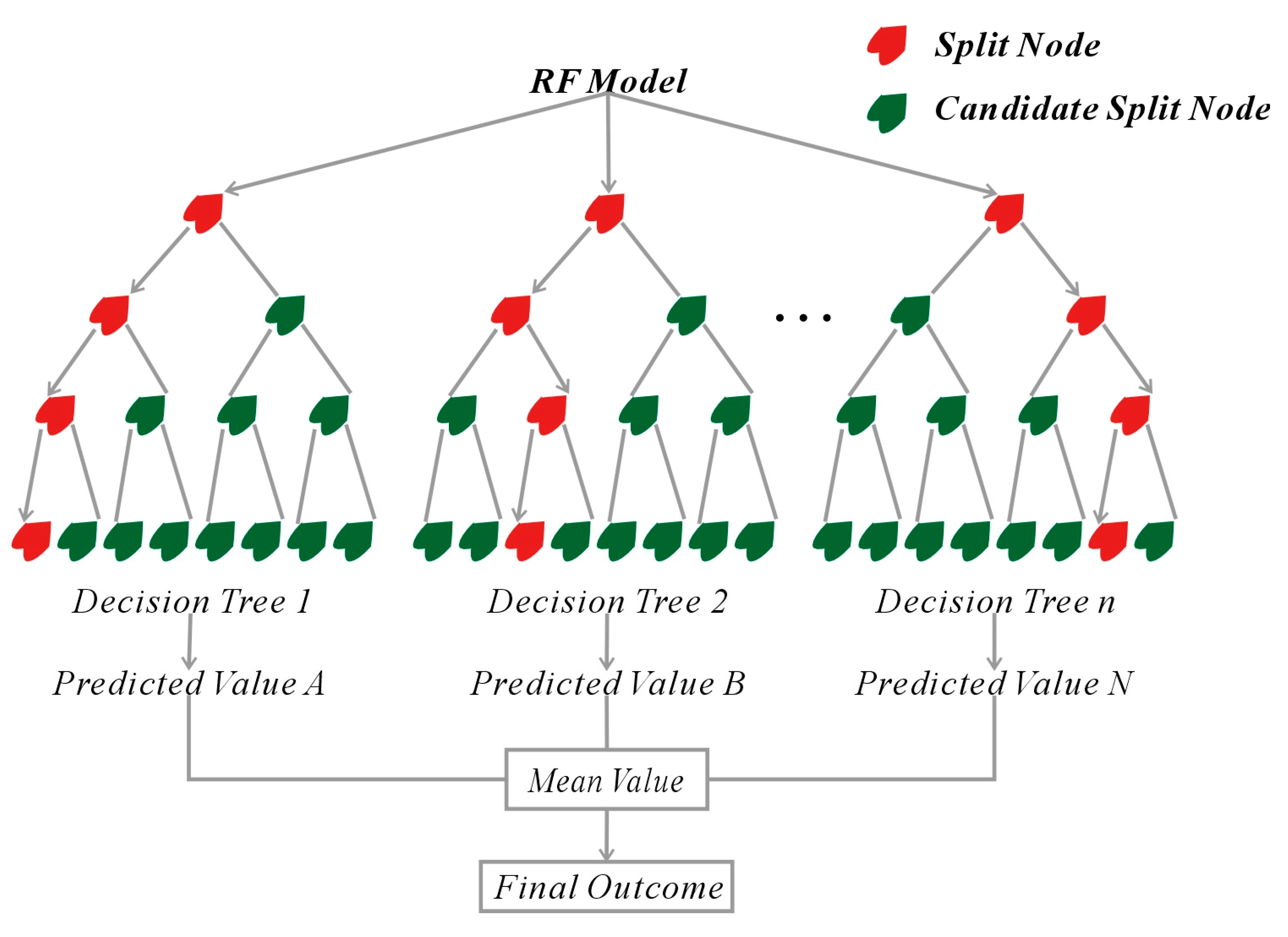
3.1.2. Random Forest Model

Random forest (RF) modeling is a bagging-type ensemble method that integrates multiple decision trees [14]. RF models randomly select samples with replacement, use specific features as inputs, and make predictions based on the average values of the decision trees. This approach is effective not only in dealing with nonlinear problems but also with numerous samples and features [13,15]. Consequently, RF models exhibit strong generalizability and void issues related to overfitting. RF modeling is implemented as follows (Figure 3):

(1)

Multiple data subsets containing K samples are created by drawing samples with replacements from the original sample set;

(2)

When each sample has N attributes, m (where m << N) attributes are randomly selected. An information-gain strategy is then applied to identify a split attribute for the given node from the m selected attributes;

(3)

Decision trees are constructed by splitting each node according to Step 2 until further splits are no longer possible;

(4)

The above steps are repeated until the desired number of decision trees has been generated;

(5)

Samples are divided into training and test sets, with factor FRs as inputs and actual states (landslide or nonlandslide) as outputs. Each decision tree predicts an outcome for each sample, which is then averaged to obtain the final regression result (Equation (2)).

$$f\left(x\right)={\displaystyle \frac{1}{M}}{\sum }_{m=1}^M f_m\left(x\right)$$

(2)

where $f\left(x\right)$ denotes the model output, $M$ represents the number of decision trees, $f_m\left(x\right)$ denotes the output of each decision tree, and $x$ represents the input evaluation factor of the RF model.

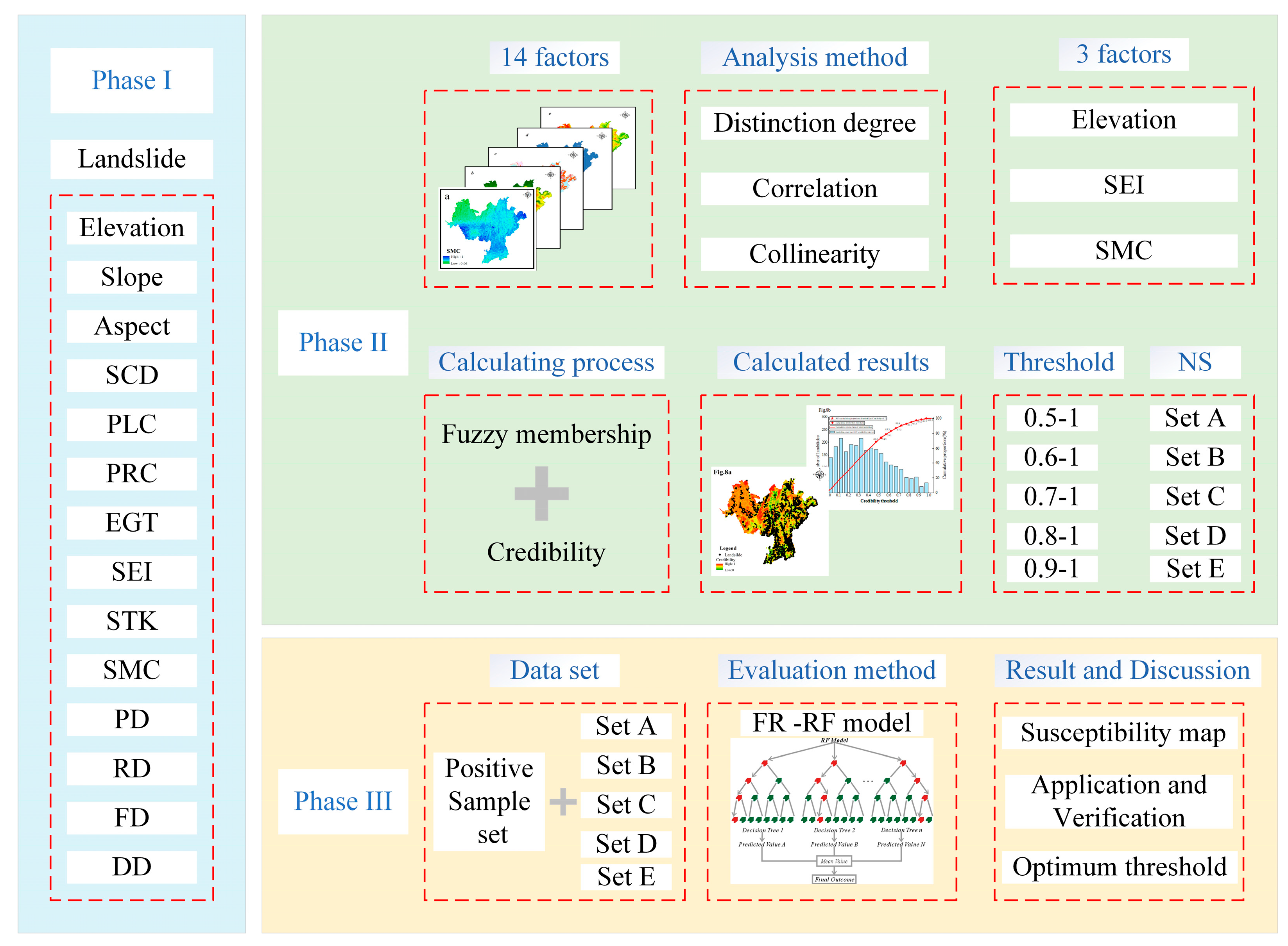
3.2. Evaluation Factor Selection Method

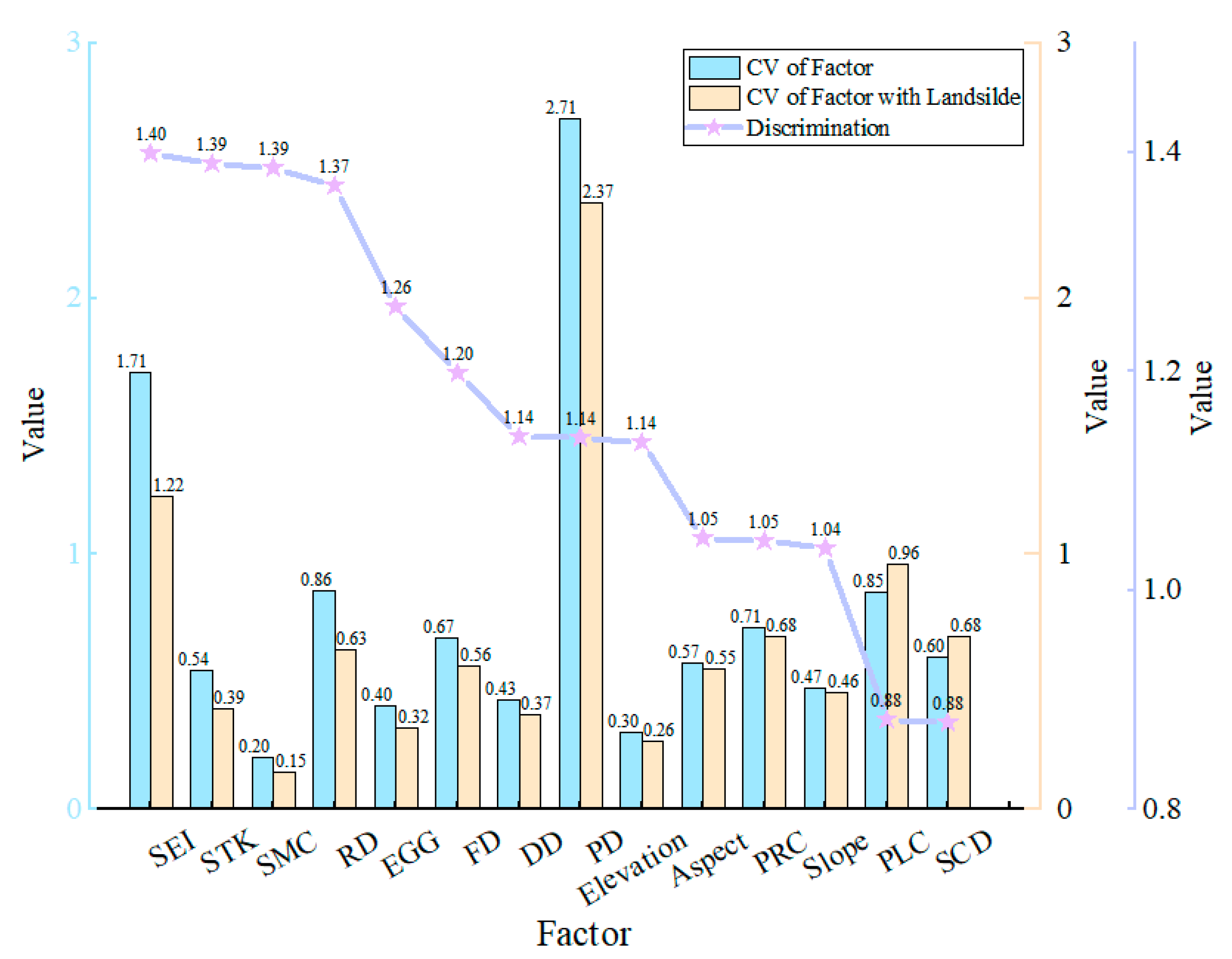
3.2.1. Differentiation

This study introduces a differentiation index to evaluate the effect of evaluation factors on landslides [16]. A higher differentiation value indicates a more significant influence on landslides, whereas a lower value suggests minimal influence [17]. The differentiation value is calculated as follows:

$$D_i={\displaystyle \frac{{CV}_{Area}}{{CV}_{Landslide}}}$$

(3)

$${CV}_i={\displaystyle \frac{{SD}_i}{{AVG}_i}}$$

(4)

where $D_i$ represents the differentiation value of the evaluation factor, and ${CV}_{Area}$ and ${CV}_{Landslide}$ denote the coefficients of variation in the evaluation factor within the study area and at the landslide, respectively; ${SD}_i$ denotes the standard deviation of the evaluation factors; and ${AVG}_i$ denotes the mean value of the evaluation factor, with $i$ representing the nonlandslide or landslide.

3.2.2. Maximum Mutual Information Coefficient Method

Mutual information quantifies the influence of the occurrence of a random event on the occurrence probability of another random event. The maximum mutual information coefficient is a statistical method for assessing the correlation between two random variables based on mutual information [18]. This statistical method is universal, equitable, and symmetric, effectively illustrating the degree of correlation between any two random variables and facilitating a deeper exploration of their relationships. The calculation process is as follows:

Let $X=\{x_1,x_2,\cdots ,x_N\}$ and $Y=\{y_1,y_2,\cdots ,y_N\}$ be two random variables. We construct an ordered pair sample set $D=\left\{\right(x_i,y_i\left)\right|i=1,2,\cdots ,N\}$ distributed in two-dimensional space, where N represents the sample size. The ranges of variables X and Y are divided into a and b subintervals, resulting in a × b grid spaces G [19]. The constraint on the total number of grids G is given by $a\times b<B\left(N\right)$, where $B\left(N\right)=N^{\phi }$ is a function of the sample size, with φ generally set between 0 and 1, typically at 0.6.

The mutual information ${\gamma }_M\left(D\right|G)$ for different grid partitioning methods can be obtained as follows:

$${\gamma }_M(D|G)={\sum }_{x\in X,y\in Y}p(x,y){\mathrm{l}\mathrm{o}\mathrm{g}}_2{\displaystyle \frac{p(x,y)}{p\left(x\right)p\left(y\right)}}$$

(5)

where $D|G$ represents the probability distribution introduced when set D is partitioned into grid space G$; p\left(x,y\right)$ denotes the joint probability density function of the random variables X and Y; and p(x) and p(y) denote the marginal probability density functions of the random variables X and Y, respectively.

Due to the existence of multiple partitioning methods for grid space G, the maximum value of ${\gamma }_M\left(D\right|G)$ under different partitioning approaches is taken as the maximum mutual information value ${\gamma }_M(D,a,b)$ for grid space G, as shown in Equation (6). To compare the maximum mutual information under different numbers of grids, it is necessary to normalize the maximum mutual information value ${\gamma }_M(D,a,b)$ of the grid space G (Equation (7)) to obtain the maximum mutual information coefficient ${\gamma }_{Z.a,b}\left(D\right)$, denoted as the most $MIC\left(D\right)$.

$${\gamma }_M(D,a,b)=max\left\{{\gamma }_M\right(D\left|G\right)\}$$

(6)

$${\gamma }_{Z.a,b}\left(D\right)={\displaystyle \frac{{\gamma }_M\left(D,a,b\right)}{{\log }_2\min \left\{a,b\right\}}},$$

(7)

$$MIC(D)=\underset{a\times b<B\left(N\right)}{max}\{{\gamma }_Z(D{)}_{a,b}\}$$

(8)

3.2.3. Collinearity Diagnosis

In landslide susceptibility modeling, it is essential to avoid multicollinearity among the evaluation factors to ensure that no factor can be nearly represented as a linear combination of others [20]. This study uses the variance inflation factor (VIF) to assess multicollinearity between the evaluation factors.

$$VIF={\displaystyle \frac{1}{1-R^2}}$$

(9)

where $R^2$ represents the coefficient of determination from the regression of other independent variables with $x_i$ as the dependent variable. A significance value of less than 0.05 and a VIF value of less than 10 indicate no multicollinearity between the evaluation factors.

3.3. Negative Sample Selection Method

3.3.1. Geographical Information Similarity

This study employs the FR method for discrete evaluation factors and the fuzzy membership method for continuous evaluation factors to calculate geographical information similarity [21,22]. The FR method, which is a standard bivariate analysis method, identifies which classification of discrete factors is more likely to contribute to landslides, as detailed in Equation (1). To ensure consistency with continuous factors, the values are normalized using Equation (10), scaling them to a range of 0–1, thereby establishing the similarity between the discrete factor classification and the factor typical classification of landslide.

$$S_{ij}={\displaystyle \frac{F{R}_{ij}-min\left(F{R}_i\right)}{max\left(F{R}_i\right)-min\left(F{R}_i\right)}}$$

(10)

where $S_{ij}$ denotes the similarity between the j-th classification of the i-th factor and the factor typical classification, $F{R}_{ij}$ denotes the FR for the j-th classification of the i-th factor, and $max\left(F{R}_i\right)$ and $min\left(F{R}_i\right)$ denote the maximum and minimum values of $F{R}_i$, respectively.

The fuzzy membership function measures the membership level of an element in a fuzzy set [23,24]. The primary advantage of the function is its ability to assign precise membership weights to fuzzy events based on the frequency of occurrence of certain events. Let there be n landslide events with the following evaluation factor values: $x_{1,},x_{2,},x_3,\dots ,x_n$. The fundamental definition of the membership function for evaluation factor x is as follows:

$$F(A_{ij})={\displaystyle \frac{A_{ij}-A_{imin}}{A_{imax}-A_{imin}}},i=\mathrm{1,2},\dots ,n$$

(11)

where $\left(A_{ij}\right)$ denotes the frequency value of landslides under the classification ${ A}_{ij}$ and $A_{ij}$ denotes the number of landslides associated with the j-th classification of the i-th factor. In contrast, $A_{imax}$ and $A_{imin}$ represent the maximum and minimum values of $A_{ij}$, respectively.

In this study, to more accurately characterize the nonlinear relationship between the evaluation factors and the landslide occurrence frequency (i.e., the relative proportion of landslides within each factor classification interval), we did not directly apply the linear normalization formula (Equation (9)). Instead, the functional relationship f(x) between the evaluation factor values and the corresponding landslide frequency was derived using the curve fitting tools in Origin software.

$$f(x)=y_0+{\displaystyle \frac{A}{w\sqrt{\pi /2}}}\mathrm{e}\mathrm{x}\mathrm{p}(-2{({\displaystyle \frac{x-x_c}{w}})}^2)$$

(12)

where $f\left(x\right)$ represents the predicted landslide frequency value corresponding to the evaluation factor x, whose mathematical expression is determined by the landslide frequency distribution pattern; $y_0$ denotes the baseline offset parameter, $A$ represents the peak area, $x_c$ denotes the peak position, and $w$ represents the peak width parameter. By applying Equation (11) to normalize the $f\left(x\right)$ function, the membership degree $S_x$ for a single evaluation factor is obtained as follows:

$$S_x={\displaystyle \frac{f\left(x\right)-min\left(f\right(x\left)\right)}{max\left(f\right(x\left)\right)-min\left(f\right(x\left)\right)}}$$

(13)

By integrating the similarity value of both discrete and continuous factors, the final geographic information similarity can be obtained as follows:

$$S=f(S_1,S_2,\cdots ,S_i,\cdots ,S_n)$$

(14)

where $S$ represents the geographical information similarity at a given location, n represents the number of evaluation factors, and $f\left(\right)$ denotes the integrated method. This study employs weighted synthesis methods.

3.3.2. Credibility Computational Method

The similarity values between the negative samples and landslide geographic environments range from 0 to 1; thus, this study employs Equation (13) to evaluate the credibility of the negative samples [25]. The resulting credibility values also span [0, 1], with higher values indicating higher credibility. Consequently, a spatial distribution map was created to demonstrate the reliability of the negative samples within the study area.

$$Reliabilit{y}_{i,j}=1-S_{i,j}$$

(15)

where $S_{i,j}$ denotes the similarity of the location at position (i, j) to the landslide geographic environment, and ${Reliability}_{i,j}$ represents the credibility of the location being identified as a negative sample.

3.4. Testing of the Evaluation Results

3.4.1. F1-Scores

The F1-score is a statistical measure of the precision of a binary grading model, which is defined as the harmonic mean of precision and recall [26]. The F1-score ranges from 0 to 1, with higher values indicating better model prediction performance. The F1-score is particularly suitable for evaluating landslide susceptibility mapping because it considers both the likelihood that a predicted landslide is accurate (precision) and that an actual landslide is correctly predicted (recall).

$$\mathrm{Precision}={\displaystyle \frac{\mathrm{T}\mathrm{P}}{\mathrm{T}\mathrm{P}+\mathrm{F}\mathrm{P}}}$$

(16)

$$\mathrm{Recall} ={\displaystyle \frac{\mathrm{T}\mathrm{P}}{\mathrm{T}\mathrm{P}+\mathrm{F}\mathrm{N}}}$$

(17)

$$F1={\displaystyle \frac{2\times \mathrm{Precision} \times \mathrm{Recall} }{ \mathrm{Precision}+ \mathrm{Recall} }}$$

(18)

where TP denotes the number of actual positive samples (correctly identified landslides), TN denotes the number of actual negative samples (correctly identified nonlandslides), FP denotes the number of false positive samples (predicted landslides that are nonlandslides), and FN denotes the number of false negative samples (predicted nonlandslides that are landslides).

3.4.2. AUC Value

The quality of susceptibility mapping can be evaluated using the AUC value. The range of AUC values is [0.5, 1]. The closer the value is to 1, the greater the ability of the model to rank the samples [27]. This value is not tied to a specific threshold; thus, it cannot accurately represent the actual performance of the model at any given threshold.

$$AUC={\displaystyle \frac{\sum _{i=1}^{\mathrm{M}}Rank\left(M_i\right)-(\mathrm{M}+1)/2}{\mathrm{M}\times \mathrm{N}}},$$

(19)

where M represents the number of positive samples; N represents the number of negative samples; and $Rank\left(M_i\right)$ denotes the sorted position of the i-th positive sample after ranking all samples (both positive and negative) in descending order based on their predicted probabilities.

4. Results

4.1. Selection of Evaluation Factors

Landslide formation is a complex process influenced by various evaluation factors. Research has demonstrated that retaining highly important but low-correlation factors can effectively minimize redundant information. Consequently, this study selects and weights the evaluation factors using differentiation, the MIC method, and collinearity diagnosis. This study then calculates the membership function of these factors to assess the credibility of the negative samples.

The 14 evaluation factors were analyzed based on differentiation. The results are presented in Figure 4. Factors with higher differentiation have a more significant influence on the landslide. To improve computational efficiency, this study established a differentiation threshold of 1.1, ultimately retaining nine evaluation factors: elevation, EGG, SEI, STK, SMC, PD, RD, DD, and FD.

This study used the MIC method, with a threshold of 0.1, to calculate the nonlinear correlation coefficients between the evaluation factors and slope conditions (Figure 5). In addition, collinearity diagnostics were performed to address multicollinearity between the evaluation factors, with thresholds set at a significance value < 0.05 and VIF > 3. The results of these calculations are presented in

Table 2. Results of collinearity diagnosis for evaluation factors.

Factor	Significance	VIF
Elevation	0	1.287
PD	0.078	1.05
SEI	0	1.02
RD	0.183	1
SMC	0	1.229

.

In summary, after conducting MIC nonlinear correlation analysis and collinearity diagnostics, seven evaluation factors were eliminated: RD, EGG, FD, DD, PD, and STK. Ultimately, three evaluation factors were retained: SEI with a weight of 0.27, elevation with a weight of 0.54, and SMC with a weight of 0.19 (Figure 6). The proportion of correlation of each factor to the total correlation sum was used as the weight for the subsequent plotting of the spatial distribution map of negative sample credibility.

4.2. Spatial Distribution Map of Negative Sample Credibility

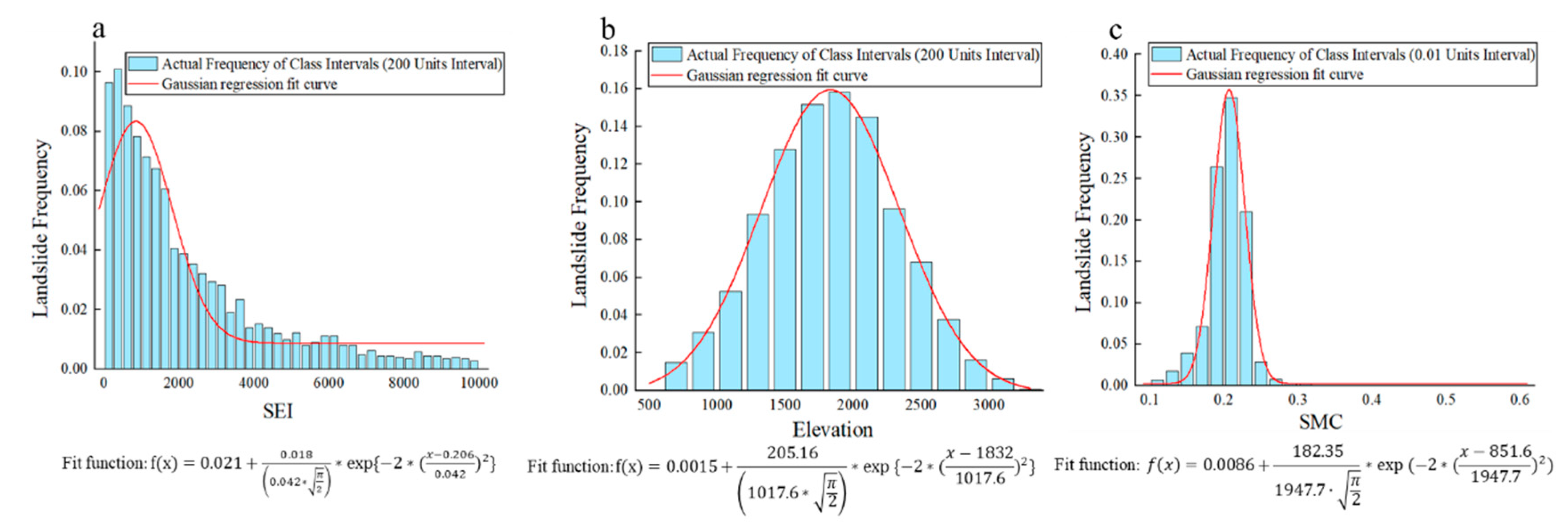
4.2.1. Calculation of the Membership Function

Based on the absence of discrete factors in the preprocessed evaluation factors, this study calculated the membership functions for the continuous evaluation factors using 2681 historical landslides in the study area. The workflow for deriving membership functions for each continuous factor was as follows. (1) Discretization and frequency calculation: Continuous evaluation factors were automatically discretized into graded intervals using Origin software 2022 landslide occurrence frequency (frequency count/total samples) within each interval was then statistically analyzed (blue histogram in Figure 7). (2) Nonlinear regression modeling: To precisely characterize the nonlinear relationship between the evaluation factors (x) and the landslide frequency (y), regression fitting via Equation (10) was applied. This established a mapping function f(x) between the median value of the graded intervals and the landslide frequency (red curve and equation in Figure 7). (3) Normalization and closed-form derivation: The normalized membership degree of f(x) was computed according to Equation (11). Piecewise closed-form expressions were then derived based on the fitting results and frequency distribution characteristics (Equations (20)–(22)).

As shown in Figure 7, the landslide-prone areas in the Liangshan Yi Autonomous Prefecture exhibit the following environmental characteristics: SEI below 850, elevation ranging between 1750 and 2250 m, and SMC between 0.18 and 0.22. Further investigation reveals that topographic constraints confine human engineering activities, resulting in SEI, elevation, and SMC exerting greater influence on landslide occurrence. In contrast, factors such as DD, fracture density, and engineering geological rock groups have relatively less impact on landslide initiation.

$$S_x=\left\{\begin{array}{c}0,\\ \exp (-2\cdot {({\displaystyle \frac{x-0.206}{0.042}})}^2),\\ 0,\end{array}\right.\begin{array}{cc}& x<0.14\\ & 0.14\le x\le 0.26\\ & x>0.26\end{array}$$

(20)

$$S_x=\exp \left(-2\times {\left({\displaystyle \frac{x-1832}{1017.6}}\right)}^2\right),$$

(21)

$$S_x=\left\{\begin{array}{c}1,\\ \exp (-2\times {({\displaystyle \frac{x-851.6}{1947.7}})}^2)\end{array}\right.\begin{array}{cc}& x<851.6\\ ,& x\ge 851.6\end{array},$$

(22)

4.2.2. Negative Sample Credibility

Equations (13) and (14) were used to perform a weighted calculation of the similarity for each evaluation factor, which yielded the overall similarity in the study region. Subsequently, the credibility of the negative samples for the entire study area was calculated using Equation (15). The credibility distribution for the negative samples in the study area is illustrated in Figure 8a. Figure 8b shows the frequency distribution for the landslide samples.

Figure 8a illustrates that landslides are primarily located in green areas with low negative sample credibility, whereas orange areas with high-credibility show very few landslides. This figure indicates that the credibility distribution map developed using the fuzzy membership credibility-integrated negative sampling method is scientifically valid and practically applicable. The negative sample credibility distribution continuity was robust and showed no significant spatial segmentation. This indicates that the map effectively captures variations in credibility and facilitates the selection of appropriate negative samples.

Figure 8b reveals that 90% of the landslides are located within the range in which the negative sample credibility is below 0.7, while only a tiny fraction are located within areas in which the credibility exceeds 0.7. This result highlights the usefulness of the credibility distribution map in rapidly selecting negative samples and assessing quality. Consequently, negative sample sets were established based on different credibility thresholds: Set A (0.5–1), Set B (0.6–1), Set C (0.7–1), Set D (0.8–1), and Set E (0.9–1). These sets are used to construct the FR–RF-coupled model.

4.3. Optimal Credibility Threshold

The ML model can autonomously adjust the weights of the evaluation factors. To reduce the risk of losing important information due to excessive removal of these factors, this study retains five evaluation factors (elevation, PD, SEI, RD, and SMC) identified through MIC nonlinear correlation analysis as inputs while using the slope state as the output. A training sample set was established using landslide and negative samples with different credibility thresholds, resulting in the development of FR–RF-coupled models (Models A–E). The predictive performance of these models was quantitatively assessed using the F1-score and AUC metrics (

Table 3. Impact analysis of the negative sample credibility threshold on FR–RF model performance.

Verification Method	Model A	Model B	Model C	Model D	Model E
Precision	0.928	0.926	0.938	0.975	0.974
Recall	0.839	0.936	0.942	0.883	0.889
F1-score	0.881	0.926	0.940	0.927	0.928
AUC	0.887	0.925	0.941	0.932	0.937

). We also calculated the ratio of landslides at each susceptibility level to the total number of landslides, denoted as A. Furthermore, we determined the ratio of the area corresponding to each susceptibility level to the total area of the study region, referred to as B. Finally, we computed the landslide ratio (B/A), as detailed in

Table 4. Susceptibility zone statistics and landslide ratio of FR–RF models.

Model	Factor	Zone I	Zone II	Zone III	Zone IV	Zone V
Model A	A	0.02	0.10	0.08	0.08	0.72
	B	0.40	0.20	0.07	0.04	0.29
	A/B	0.05	0.51	1.10	1.89	2.47
Model B	A	0.03	0.03	0.10	0.09	0.76
	B	0.44	0.09	0.09	0.06	0.32
	A/B	0.06	0.34	1.07	1.46	2.38
Model C	A	0.02	0.03	0.04	0.10	0.82
	B	0.38	0.08	0.08	0.10	0.37
	A/B	0.05	0.36	0.51	1.00	2.24
Model D	A	0.04	0.04	0.03	0.04	0.85
	B	0.37	0.09	0.04	0.04	0.45
	A/B	0.10	0.43	0.84	0.90	1.88
Model E	A	0.04	0.03	0.03	0.02	0.88
	B	0.38	0.07	0.03	0.02	0.50
	A/B	0.10	0.45	1.03	0.99	1.77

Zones I–V: very low/low/medium/high/very high; A: landslide proportion, B: area proportion, and A/B: landslide ratio.

.

Table 3 indicates that as the credibility of the negative samples increases, the precision of the model increases and stabilizes. This suggests that in the early stages of enhancing the credibility of the negative samples, the model reduces the misclassification of the negative samples, thereby decreasing the FP. However, as the credibility of the negative samples continues to improve, the precision does not continue to improve indefinitely due to the limitations of the model. The recall rate initially increases and then decreases, indicating that in the early stages of enhancing the credibility of negative samples, the model reduces the misclassification of positive samples, which decreases the number of FN. However, as the credibility of the negative samples improves, to reduce the FP, the model increases the identification threshold of positive samples, thereby increasing the FN. Thus, establishing a suitable credibility threshold range is essential.

This study employs the F1-score and AUC as evaluation metrics to identify an appropriate credibility threshold. Model C achieved the highest F1-score among the coupled models, indicating a lower omission rate (high recall) and a lower FP rate (high precision). Model C also exhibited the highest AUC value, demonstrating an effective balance between sensitivity and specificity, high global ranking performance, and strong discriminative ability.

Further analysis indicates that when the credibility thresholds are set to 0.5–1 (Model A) and 0.6–1 (Model B), mixed negative and positive samples are obtained, resulting in reduced and unstable quality of negative samples. This makes it difficult for the model to distinguish between the samples, leading to poor global ranking and overall balancing ability. In contrast, with credibility thresholds of 0.8–1 (Model D) or 0.9–1 (Model E), the negative and positive samples exhibited significantly different characteristics. This allows the model to distinguish between them accurately and achieve very high accuracy. However, the negative samples only represent the typical characteristics of nonlandslide areas in the study area. The model may increase the high-susceptibility zone by lowering the classification threshold, which may result in FP and an overestimation of susceptibility in the study area. In conclusion, the optimal threshold for selecting negative samples in the study area is 0.7–1 (Model C).

Based on the dual principles of minimizing the area proportions of the high-/very-high-susceptibility zones and maximizing the concentration of landslide distribution (landslide ratio), this study comprehensively ranked the candidate models. The area proportions of the high-/very-high-susceptibility zones across the models were ranked in descending order as follows: Model E (0.52) > Model D (0.49) > Model C (0.47) > Model B (0.38) > Model A (0.36). The landslide ratios in areas of high and extremely high susceptibility for each model, ranked from highest to lowest (Table 4), are as follows: Model C (0.92) > Model E (0.90) > Model D (0.89) > Model B (0.85) > Model A (0.80). Based on further analysis, only Models B, C, and D strictly comply with the distribution requirement that the landslide ratio value increases monotonically with susceptibility levels and exhibits high concentrations in higher-susceptibility zones (high and very high). Through a comprehensive analysis of these indicators and their conformity to the distribution patterns, Model C, constructed by selecting negative samples within the credibility threshold range of 0.7–1, was identified as the optimal landslide susceptibility evaluation model. Model C not only demonstrates exceptional performance (high-credibility differentiation ability) and reliability within this threshold but also produces the most rational susceptibility zoning results (Figure 9), namely, high- and very-high-susceptibility zones occupy a moderate proportion (47%), while concentrating the vast majority of historical landslide events (92%) in the study area.

Based on the optimal model (Model C), this study generated a high-precision spatial distribution map of landslide susceptibility (Figure 9). The map intuitively reveals that landslides in the study area are predominantly concentrated in zones of higher susceptibility grades (high- and very-high-susceptibility zones), with marked spatial heterogeneity providing direct evidence for identifying landslide risk hotspot areas. These results effectively balance model performance and the geoscientific characteristics of landslide distribution, thereby providing robust spatial information support for developing scientific and rational landslide risk prevention measures in the study area.

5. Discussion

5.1. Comparative Analysis of Application Effects and Novel Approach Advantages in Negative Sampling Methods

Distinct negative sample selection methods significantly impact the quality of negative samples. To rigorously validate the effectiveness of the proposed sampling approach, this study generated spatial distribution maps of negative landslide samples using the geographic similarity-based sampling method (Figure 10a) and the FR model sampling method (Figure 10b) [9,28].

Figure 10a shows the credibility distribution map of the negative samples, which was created by integrating the kernel density of the evaluation factors within a search radius of 500 m. The map illustrates that regions with a higher density of landslides correspond to the lower credibility of negative samples, whereas areas with a lower density of landslides demonstrate higher credibility. Although this method successfully confines low-credibility areas to those adjacent to near landslides, it fails to map the environmental feature space defined by evaluation factors throughout the study area, inadequately reflecting the distribution characteristics of potential landslides. Figure 10b shows the landslide susceptibility map constructed using the FR model. Using the constructed map to select negative samples from low-susceptibility areas has several limitations. First, the FR values of the evaluation factors are not continuous, which leads to low continuity in the landslide susceptibility map and pronounced spatial patchiness, thereby complicating the selection of negative samples. Second, classifying landslide susceptibility involves subjectivity; this study categorizes the susceptibility of the study area into five levels with intervals of 0.2. Most areas are classified as extremely low or low susceptibility, but they also contain many historical landslides, which results in the quality of negative samples not being guaranteed.

Although methods such as geographic environmental similarity and FR model sampling primarily address the spatial delineation of “where to select” negative samples (i.e., defining nonlandslide areas), a quantitative evaluation standard for the “reliability” of selected samples is yet to be established for these models. This limitation impedes the systematic analysis of the effect of variations in negative sample quality on the performance of landslide susceptibility assessment models [4,29]. In contrast, the proposed fuzzy membership-based credibility sampling method achieves a fundamental breakthrough: it pioneers an intuitive and quantitative expression of negative sample reliability through “credibility” metrics. By generating a spatially continuous credibility distribution map, the proposed approach not only reveals the quality gradients of negative samples across regions but also provides an objective basis for screening high-quality samples (i.e., high-credibility samples). The proposed method significantly enhances both the theoretical foundation and operational feasibility of producing high-precision landslide susceptibility maps.

5.2. Application and Validation Based on Machine Learning Models

We also used a support vector machine (SVM) model to evaluate the effects of negative samples with different credibility thresholds on ML performance. Using the negative sample sets (A–E) and positive samples (landslide samples) described in Section 4.2.2, we developed FR-SVM-coupled models (models a–e). The validation results of the models are summarized in

Table 5. Validation of FR-SVM performance under negative sample credibility thresholds.

Verification Method	Model a	Model b	Model c	Model d	Model e
Precision	0.855	0.854	0.938	0.946	0.966
Recall	0.891	0.912	0.942	0.896	0.792
F1 score	0.873	0.882	0.940	0.920	0.870
AUC	0.872	0.885	0.939	0.902	0.874

.

Table 5 demonstrates that the evaluation metrics of the FR-SVM-coupled models are closely aligned with those of the FR–RF-coupled models. Both models achieve optimal performance when the credibility threshold range for negative samples is 0.7–1. This result suggests that the negative sample credibility distribution map constructed using the proposed method demonstrates a level of universality, providing a dependable foundation for selecting negative samples for landslide research in the study area [30]. In addition, as shown in Table 3 and Table 5, the evaluation metrics of the FR-SVM-coupled models exhibit more substantial variations than those of the FR–RF-coupled models as the credibility threshold for negative samples changes. Furthermore, the optimal prediction values of the FR-SVM-coupled models were slightly lower than those of the FR–RF-coupled models. This result indicates that the stability and predictive capability of the FR–RF-coupled models are superior [3,15]. In future research, the authors will explore the application of various ML models for landslide susceptibility mapping in the study area to enhance assessment precision.

5.3. Limitations and Future Directions

Although the proposed fuzzy membership-based credibility quantification method for negative samples exhibits significant advantages in terms of enhancing representational capacity (spatial continuity and reflection of potential landslide distribution) and achieving quantitative reliability assessment of negative samples, several noteworthy limitations remain to be addressed in future research:

The construction of negative sample credibility maps inherently heavily relies on the selected evaluation factors (in this study: elevation, SEI, and SMC). Although the factor selection process was optimized by rigorous discriminative power analysis, nonlinear correlation assessment, and collinearity diagnostics, this dependency is unavoidable because credibility is computed within the environmental space defined by these factors [14,31]. Consequently, significant changes in the geological–geographical settings, dominant landslide mechanisms, or key triggering factors of a study area may necessitate re-evaluation and screening of the most relevant evaluation factors to ensure the validity of the constructed credibility map. Future research should validate the proposed approach across more diverse regions and explore the establishment of adaptive factor screening frameworks that respond to region-specific controlling factors.

The core of the proposed method lies in constructing fuzzy membership functions by fitting the functional relationships between the evaluation factors and the landslide frequency, thereby integrating the statistical patterns into fuzzy theory [32]. However, the selection of optimal function forms (e.g., linear, sigmoid, and Gaussian) and the parameter determination process introduce subjectivity [24]. Different functional forms may yield subtle variations in the credibility computation results. Although this study aimed to capture nonlinear relationships between factors and negative samples, establishing more objective and robust fuzzy membership functions to reduce uncertainty due to subjectivity remains a critical issue that warrants in-depth exploration in future research.

Although the proposed negative sample sampling method demonstrates universal applicability across two mainstream ML models, namely, SVM and RF, with consistent optimal threshold intervals, significant differences exist in their responsiveness to negative sample quality variations (e.g., RF exhibits superior stability and predictive capability). This indicates that the precision and robustness of the final landslide susceptibility mapping results are significantly influenced by the inherent characteristics of the selected ML model. These findings imply that extensively adopted general-purpose ML models (e.g., SVM and RF) exhibit substantial disparities in capturing the intrinsic complex spatial dependencies and multisource data integration requirements of landslide susceptibility assessment [33]. Consequently, there is an urgent need for an in-depth exploration of the application efficacy of diverse ML models in this domain [34].

6. Conclusions

(1)

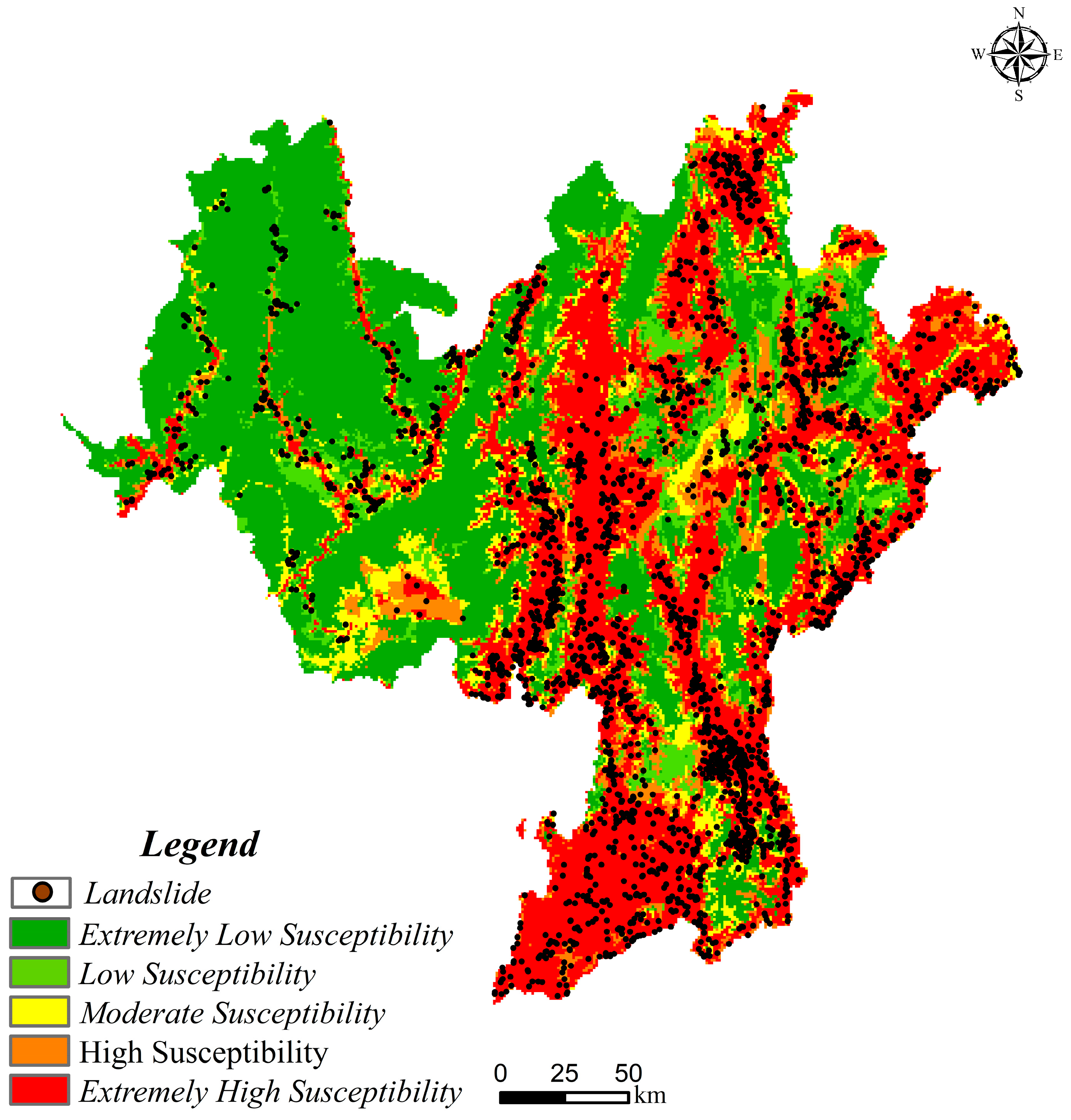
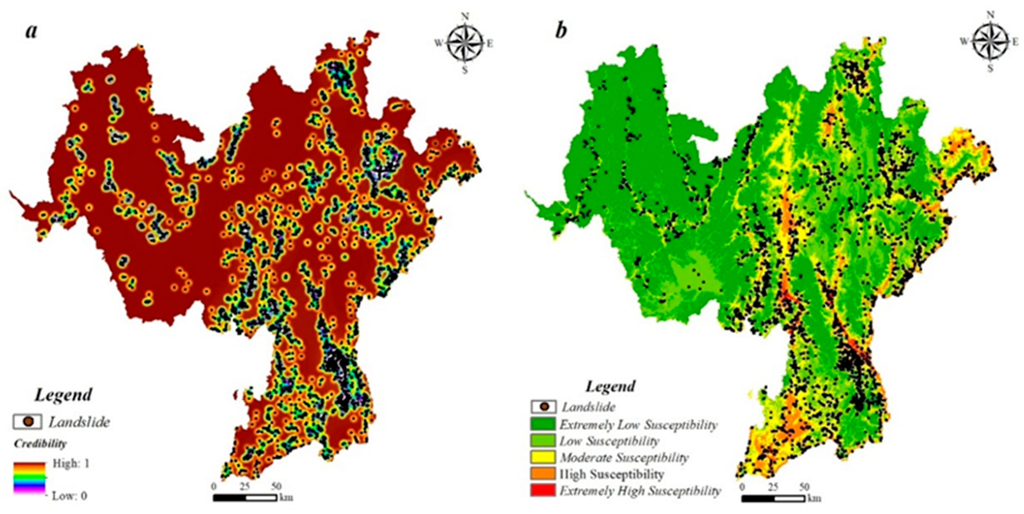
This study successfully developed and applied a fuzzy membership-based method for calculating negative sample credibility for landslide susceptibility assessment. The proposed approach triggers a paradigm shift: from defining “where to select negative samples” to quantitatively evaluating “how reliable the selected samples are.” The proposed method not only overcomes the significant limitations of conventional sampling methods (such as inadequate spatial continuity and fragmented representations of environmental feature spaces) but also establishes an intuitive and quantifiable reliability metric (i.e., credibility) for negative landslide samples. The resulting credibility distribution map of the negative samples exhibits exceptional spatial continuity and effectively characterizes the nonlandslide spatial patterns, thereby substantially enhancing the scientific rigor and reliability of negative sample selection. Crucially, the proposed method provides robust theoretical and operational support for constructing high-precision landslide susceptibility models;

(2)

Systematic validation using SVM and RF models confirms that negative samples with credibility thresholds in the 0.7–1.0 range represent the optimal choice for balancing model performance and landslide distribution characteristics. Selecting negative samples within this threshold range enables the generation of scientifically robust landslide susceptibility maps. The results were systematically validated across two distinct ML models, demonstrating the broad applicability of the credibility mapping framework and the proposed sampling methodology. The proposed approach establishes a robust theoretical framework for selecting reliable negative samples in the study area and analogous regions;

(3)

The primary contribution of this study lies in its pioneering application of fuzzy membership theory to spatialized quantitative representation of negative sample credibility, which provides a novel and effective technical solution to the long-standing challenge of negative sample quality in landslide susceptibility modeling. The generated continuous, high-resolution credibility distribution map deepens our understanding of the spatial heterogeneity in “nonlandslide areas” and its latent association with landslide occurrence mechanisms. This result provides a reliable tool for geoscientists to select high-credibility negative samples and provides critical technical support for disaster managers in generating high-fidelity susceptibility maps and robust scientific foundations for land-use planning and disaster risk reduction policy formulation across diverse regions.

References

1. Lu, J.; He, Y.; Zhang, L.; Zhang, Q.; Tang, J.; Huo, T.; Zhang, Y. A synergistic CNN-DF method for landslide susceptibility assessment. IEEE J. Sel. Top. Appl. Earth Obs. Remote Sens. 2025, 18, 6584–6599. [Google Scholar] [CrossRef]
2. Tekin, S.; Quesada Román, A.; Çan, T. Landslide susceptibility assessment of the Asi watershed, southern Türkiye. Turk. J. Earth Sci. 2024, 33, 208–223. [Google Scholar] [CrossRef]
3. Kudaibergenov, M.; Nurakynov, S.; Iskakov, B.; Iskaliyeva, G.; Maksum, Y.; Orynbassarova, E.; Akhmetov, B.; Sydyk, N. Application of Artificial Intelligence in Landslide Susceptibility Assessment: Review of Recent Progress. Remote Sens. 2025, 17, 34. [Google Scholar] [CrossRef]
4. Zhu, Y.; Liu, S.; Yin, K.; Zeng, T.; Guo, Z.; Liu, Z.; Yang, H. Impact of negative sampling strategies on landslide susceptibility assessment. Adv. Space Res. 2025. [Google Scholar] [CrossRef]
5. Li, M.; Tian, H. Insights from Optimized Non-Landslide Sampling and SHAP Explainability for Landslide Susceptibility Prediction. Appl. Sci. 2025, 15, 1163. [Google Scholar] [CrossRef]
6. Fu, Y.; Fan, Z.; Li, X.; Wang, P.; Sun, X.; Ren, Y.; Cao, W. The Influence of Non-Landslide Sample Selection Methods on Landslide Susceptibility Prediction. Land 2025, 14, 722. [Google Scholar] [CrossRef]
7. Zhang, Q.; He, Y.; Zhang, Y.; Lu, J.; Zhang, L.; Huo, T.; Tang, J.; Fang, Y.; Zhang, Y. A Graph–Transformer Method for Landslide Susceptibility Mapping. IEEE J. Sel. Top. Appl. Earth Obs. Remote Sens. 2024, 17, 14556–14574. [Google Scholar] [CrossRef]
8. Ke, C.; Sun, P.; Zhang, S.; Li, R.; Sang, K. Influences of non-landslide sampling strategies on landslide susceptibility mapping: A case of Tianshui city, Northwest of China. Bull. Eng. Geol. Environ. 2025, 84, 123. [Google Scholar] [CrossRef]
9. Guo, Z.; Tian, B.; Zhu, Y.; He, J.; Zhang, T. How do the landslide and non-landslide sampling strategies impact landslide susceptibility assessment?—A catchment-scale case study from China. J. Rock Mech. Geotech. Eng. 2024, 16, 877–894. [Google Scholar] [CrossRef]
10. Jiang, W.; Li, L.; Niu, R. Impact of Non-Landslide Sample Sampling Strategies and Model Selection on Landslide Susceptibility Mapping. Appl. Sci. 2025, 15, 2132. [Google Scholar] [CrossRef]
11. Li, M.; Li, L.; Lai, Y.; He, L.; He, Z.; Wang, Z. Geological Hazard Susceptibility Analysis Based on RF, SVM, and NB Models, Using the Puge Section of the Zemu River Valley as an Example. Sustainability 2023, 15, 11228. [Google Scholar] [CrossRef]
12. Ahmed, S.; Fatma, O.; Yacine, S.; Fatna, M.; Youcef, B.; Said, G.M. Statistical-based methods for landslides susceptibility mapping in the Wilaya of Mila (northeast Algeria). J. Earth Syst. Sci. 2025, 134, 21. [Google Scholar] [CrossRef]
13. Pham, B.T.; Vu, V.D.; Costache, R.; Phong, T.V.; Ngo, T.Q.; Tran, T.-H.; Nguyen, H.D.; Amiri, M.; Tan, M.T.; Trinh, P.T.; et al. Landslide susceptibility mapping using state-of-the-art machine learning ensembles. Geocarto Int. 2025, 37, 5175–5200. [Google Scholar] [CrossRef]
14. Huang, F.; Liu, K.; Jiang, S.; Catani, F.; Liu, W.; Fan, X.; Huang, J. Optimization method of conditioning factors selection and combination for landslide susceptibility prediction. J. Rock Mech. Geotech. Eng. 2025, 17, 722–746. [Google Scholar] [CrossRef]
15. Huang, F.; Yang, Y.; Jiang, B.; Chang, Z.; Zhou, C.; Jiang, S.-H.; Huang, J.; Catani, F.; Yu, C. Effects of different division methods of landslide susceptibility levels on regional landslide susceptibility mapping. Bull. Eng. Geol. Environ. 2025, 84, 276. [Google Scholar] [CrossRef]
16. Mirus, B.B.; Belair, G.M.; Wood, N.J.; Jones, J.; Martinez, S.N. Parsimonious High-Resolution Landslide Susceptibility Modeling at Continental Scales. AGU Adv. 2024, 5, e2024AV001214. [Google Scholar] [CrossRef]
17. Ning, Z.; Tie, Y.; Sun, C.; Xu, W. Geohazard susceptibility mapping considering spatial heterogeneity: A case study of Xide County in Sichuan Province. Nat. Hazards 2024. [Google Scholar] [CrossRef]
18. Aldiansyah, S.; Wardani, F. Assessment of resampling methods on performance of landslide susceptibility predictions using machine learning in Kendari City, Indonesia. Water Pract. Technol. 2024, 19, 52–81. [Google Scholar] [CrossRef]
19. Tan, S.-Q.; Zhang, X.; Li, Q.; Ai, C. Information push model-building based on maximum mutual information coefficient(Article). J. Jilin Univ. 2018, 48, 558–563. [Google Scholar] [CrossRef]
20. Dunlong, L.; Qian, X.; Xuejia, S.; Shaojie, Z.; Hongjuan, Y. Landslide susceptibility prediction method based on HSOM and IABPA-CNN in Wenchuan earthquake disaster area. J. Mt. Sci. 2024, 21, 4001–4018. [Google Scholar]
21. Hong, H.; Wang, D.; Zhu, A.-X.; Wang, Y. Landslide susceptibility mapping based on the reliability of landslide and non-landslide sample. Expert Syst. Appl. 2024, 243, 122933. [Google Scholar] [CrossRef]
22. Xiao, Y.; Li, G.; Wei, L.; Ding, J.; Zhang, Z. Landslide Susceptibility Assessment Using the Geographical-Optimal-Similarity Model. Appl. Sci. 2025, 15, 1843. [Google Scholar] [CrossRef]
23. Baharvand, S.; Rahnamarad, J.; Soori, S.; Saadatkhah, N. Landslide susceptibility zoning in a catchment of Zagros Mountains using fuzzy logic and GIS. Environ. Earth Sci. 2020, 79, 204. [Google Scholar] [CrossRef]
24. Oleng, M.; Ozdemir, Z.; Pilakoutas, K. Co-seismic and rainfall-triggered landslide hazard susceptibility assessment for Uganda derived using fuzzy logic and geospatial modelling techniques. Nat. Hazards 2024, 120, 14049–14082. [Google Scholar] [CrossRef]
25. Xu, Q.; Li, W.; Liu, J.; Wang, X. A geographical similarity-based sampling method of non-fire point data for spatial prediction of forest fires. For. Ecosyst. 2023, 10, 195–214. [Google Scholar] [CrossRef]
26. Zhao, P.; Wang, Y.; Xie, Y.; Uddin, M.G.; Xu, Z.; Chang, X.; Zhang, Y. Landslide susceptibility assessment using information quantity and machine learning integrated models: A case study of Sichuan province, southwestern China. Earth Sci. Inform. 2025, 18, 190. [Google Scholar] [CrossRef]
27. Cao, W.-g.; Fu, Y.; Dong, Q.-y.; Wang, H.-g.; Ren, Y.; Li, Z.-y.; Du, Y.-y. Landslide susceptibility assessment in Western Henan Province based on a comparison of conventional and ensemble machine learning. China Geol. 2023, 6, 409–419. [Google Scholar]
28. Khabiri, S.; Crawford, M.M.; Koch, H.J.; Haneberg, W.C.; Zhu, Y. An Assessment of Negative Samples and Model Structures in Landslide Susceptibility Characterization Based on Bayesian Network Models. Remote Sens. 2023, 15, 3200. [Google Scholar] [CrossRef]
29. Wang, J.; Wang, Y.; Li, M.; Qi, Z.; Li, C.; Qi, H.; Zhang, X. Improved landslide susceptibility assessment: A new negative sample collection strategy and a comparative analysis of zoning methods. Ecol. Indic. 2024, 169, 112948. [Google Scholar] [CrossRef]
30. Huang, F.; Teng, Z.; Yao, C.; Jiang, S.-H.; Catani, F.; Chen, W.; Huang, J. Uncertainties of landslide susceptibility prediction: Influences of random errors in landslide conditioning factors and errors reduction by low pass filter method. J. Rock Mech. Geotech. Eng. 2024, 16, 213–230. [Google Scholar] [CrossRef]
31. Shu, H.; Qi, S.; Liu, X.; Shao, X.; Wang, X.; Sun, D.; Yang, S.; He, J. Relationship between continuous or discontinuous of controlling factors and landslide susceptibility in the high-cold mountainous areas, China. Ecol. Indic. 2025, 172, 113313. [Google Scholar] [CrossRef]
32. Sun, X.; Yuan, L.; Tao, S.; Liu, M.; Li, D.; Zhou, Y.; Shao, H. A novel landslide susceptibility optimization framework to assess landslide occurrence probability at the regional scale for environmental management. J. Environ. Manag. 2022, 322, 116108. [Google Scholar] [CrossRef] [PubMed]
33. Topaçli, Z.K.; Ozcan, A.K.; Gokceoglu, C. Performance Comparison of Landslide Susceptibility Maps Derived from Logistic Regression and Random Forest Models in the Bolaman Basin, Türkiye. Nat. Hazards Rev. 2024, 25, 04023054. [Google Scholar] [CrossRef]
34. Xu, W.; Xu, W.; Cui, Y.; Wang, J.; Gong, L.; Zhu, L. Landslide susceptibility zoning with five data models and performance comparison in Liangshan Prefecture, China. Front. Earth Sci. 2024, 12, 1417671. [Google Scholar] [CrossRef]
Figure 1. Geographic overview and landslide distribution in the Liangshan Yi Autonomous Prefecture.
Applsci 15 07646 g001
Figure 2. Workflow of the sampling method based on fuzzy membership credibility for landslide susceptibility assessment.
Applsci 15 07646 g002
Figure 3. Flowchart of RF model construction and prediction.
Applsci 15 07646 g003
Figure 4. Preliminary selection results of evaluation factors based on the discrimination threshold.
Applsci 15 07646 g004
Figure 5. Nonlinear correlation analysis between evaluation factors and the slope state.
Applsci 15 07646 g005
Figure 6. Selected evaluation factors: (a) SEI; (b) elevation; and (c) SMC.
Applsci 15 07646 g006
Figure 7. Relationships and fitting curves between evaluation factors and landslide frequency: (a) SEI; (b) elevation; and (c) SMC.
Applsci 15 07646 g007
Figure 8. Spatial credibility distribution of negative samples based on fuzzy membership and its validation with landslide samples. (a) Spatial distribution of negative sample credibility. (b) Distribution and cumulative proportion of landslides across credibility intervals.
Applsci 15 07646 g008
Figure 9. Landslide susceptibility refined assessment map of the study area based on the optimal model (Model C).
Applsci 15 07646 g009
Figure 10. Spatial manifestations of two negative sample sampling strategies: (a) geographic environmental similarity sampling and (b) FR model sampling.
Applsci 15 07646 g010