AI-Driven Belt Failure Prediction and Prescriptive Maintenance with Motor Current Signature Analysis

Abstract

Industrial belt failures pose significant challenges to manufacturing operations, often resulting in costly downtime and maintenance interventions. This study presents a comprehensive approach to belt failure analysis, leveraging advanced monitoring and diagnostic techniques. Through the integration of motor current signature analysis (MCSA) and machine learning algorithms, particularly long short-term memory (LSTM) networks, this study aims to predict and detect belt degradation in real time. The methodology involves the collection and pre-processing of raw spectral data from industrial assets, followed by the training and optimization of predictive models. The effectiveness of the approach is demonstrated through extensive testing against real-world data, showcasing its ability to accurately forecast belt failures and enable proactive maintenance strategies. The results obtained from the testing phase reveal a high level of accuracy in predicting belt failures, with the developed models consistently outperforming traditional methods. The incorporation of LSTM networks and swarm intelligence algorithms led to a significant improvement in predictive capabilities, allowing for the early detection of degradation patterns and timely intervention. By harnessing the power of data-driven predictive analytics, the research offers a promising pathway towards enhancing operational efficiency and minimizing unplanned downtime in industrial settings. This study not only contributes to the field of predictive maintenance but also underscores the transformative potential of advanced monitoring technologies in optimizing asset reliability and performance.

1. Introduction

The vast majority of industrial operations rely on induction motors. Their robust construction, stemming from the absence of brushes and commutators, makes them the preferred choice across a wide range of applications. As these machines power most industrial loads, any failure in their components can become a critical bottleneck, leading to operational delays and economic losses.

Three-phase induction motors are extensively employed across industrial sectors due to their high reliability, energy efficiency, low maintenance requirements, and straightforward construction [1,2]. These attributes make them essential in applications such as manufacturing, automation, and energy systems.

Structurally, an induction motor comprises the following two main components: the stator and the rotor. The stator, energized by an alternating current (AC), generates a rotating magnetic field. This field induces an electric current in the rotor, which in turn creates a secondary magnetic field. The interaction between these fields produces torque, causing the rotor to rotate and provide mechanical power to external systems [3,4].

Despite their robustness, induction motors remain susceptible to faults that can com-promise operational continuity. Among these, belt failures are particularly frequent in motor-driven systems that rely on belt–pulley mechanisms for power transmission [5,6]. Such failures can lead to mechanical unbalances, decreased efficiency, unscheduled down-time, and increased maintenance costs. Belt degradation manifests itself in several forms, including misalignment, slippage, tension loss, fraying, cracking, and material fatigue, often results from prolonged operation, harsh environments, or improper setup [7,8].

Given the critical role that belts play, the early detection and prediction of belt-related faults have become a priority in industrial maintenance. Advances in sensing technologies and data analytics have enabled the transition from reactive to predictive maintenance strategies. In particular, the use of machine learning techniques has shown promise in forecasting equipment degradation and preventing failures before they occur.

Among these techniques, artificial neural networks (ANNs)—especially deep learning architectures such as recurrent neural networks (RNNs) and long short-term memory (LSTM) networks—have demonstrated strong performance in modeling time-dependent patterns within complex, non-linear, and noisy datasets [9]. These models eliminate the need for extensive manual feature extraction and have been successfully applied in various prognostic applications. However, most existing approaches target general motor faults or rely on processed vibration signals, often neglecting the potential of electrical data to identify mechanical issues such as belt wear.

This study aims to address this gap. We propose a time-domain forecasting framework for the early detection of belt degradation using electrical data captured by embedded sensors. The methodology begins with a statistical baseline model (ARIMA) [10,11] and evolves toward a more advanced deep learning approach, specifically LSTM networks [12,13]. The objective is to develop a dynamic, robust, and practical tool capable of predicting belt failure with high accuracy, contributing to smarter maintenance planning and reduced operational risk in the industry.

2. Motor Fault Diagnosis and Prediction

2.1. The Problem of Fault Diagnosis

Fault detection and diagnosis in electric motors are key enablers for predictive maintenance strategies. As motor-driven systems become more complex and critical, the early identification of anomalies is essential to avoid costly failures and downtime. A typical diagnosis process is structured into the following four stages: signal acquisition, signal processing, fault detection, and fault classification [14,15].

The first step involves acquiring signals such as current, voltage, or vibration, typically using non-invasive sensors. Once collected, these signals are preprocessed to enhance relevant features and suppress noise. In the detection stage, anomalies are identified based on deviations from expected patterns, which are then classified to determine fault type, severity, and location.

Faults in electric motors manifest through changes in electrical behavior and are often subtle and masked by operational variability. This complexity necessitates advanced diagnostic methods capable of extracting meaningful patterns from noisy and dynamic data streams. The challenge lies not only in detecting these anomalies, but also in predicting their evolution over time [16].

2.2. Motor Current Signature Analysis

Motor current signature analysis (MCSA) is a widely used condition monitoring technique that evaluates the frequency components of stator current signals to infer motor health. It is particularly attractive due to its non-intrusive nature, requiring no mechanical disassembly or additional instrumentation beyond current sensors [17].

The presence of faults, electrical or mechanical, introduces characteristic frequency components into the motor current. These frequencies arise from phenomena such as rotor asymmetry, load unbalances, or mechanical misalignment, which disturb the magnetic field and alter the current waveform. By applying spectral analysis, often via Fast Fourier Transform (FFT), these fault signatures can be isolated and monitored over time [18].

The effectiveness of MCSA lies in its ability to detect both localized defects and systemic issues. However, its accuracy depends on consistent operating conditions, as variations in load or supply can affect signal interpretation. Despite this, it remains a foundational method in motor diagnostics and is particularly effective when combined with data-driven analysis techniques [9,14].

LSTM

Long short-term memory (LSTM) networks are a specialized type of recurrent neural network (RNN) designed to model sequential data with long-range dependencies. Traditional RNNs often suffer from vanishing gradient issues when learning from extended time sequences. LSTMs address this limitation through the use of memory cells and gating mechanisms that regulate information flow [19].

In the LSTM structure, f_t, i_t, and o_t are three gates designed to control the flow of information. f_t controls the information of the memory cells from t − 1 to time t. i_t controls the input of information into the memory cells at time t. In the end, o_t controls the information of the memory cells at time t in the hidden state of h_t. These are shown in the following equation:

$$f_t=\sigma \left(w_{f_c}{C}_{t-1}+w_{f_h}{h}_{t-1}+w_{f_x}{x}_t+b_f\right)$$

(1)

$$i_t=\sigma \left(w_{i_c}{C}_{t-1}+w_{i_h}{h}_{t-1}+w_{i_x}{x}_t+b_i\right)$$

(2)

$$o_t=\sigma \left(w_{o_c}{C}_{t-1}+w_{o_h}{h}_{t-1}+w_{o_x}{x}_t+b_o\right)$$

(3)

where w_fc, w_ih, and w_oh are the weight matrices between gate f_t and memory cell C_t−1, and b _f is the bias of the gate f_t. Other weight matrices are derived as follows: C_t and C_t−1 represent the values of memory cells at time t and time t − 1, b_f, b_i, and b_o represent the biases, and σ is the activation function. The structure of the unit of the long short-term memory network is shown in Figure 1.

In predictive maintenance contexts, LSTMs are highly effective for modeling time series data such as vibration levels, current amplitudes, or frequency domain features. Their strength lies in capturing nonlinear temporal trends and forecasting future signal evolution based on past behavior. This makes them well-suited for predicting gradual degradation processes that precede fault events.

3. Related Work

The concept of maintenance has evolved over time, due to developments in research and maintenance policies related to the realities of institutions, ensuring the efficiency, quality, and availability of assets [14].

Maintenance strategies in industrial systems are traditionally classified into corrective, preventive, and predictive approaches. Each reflects a different balance between operational risk, cost, and system reliability.

Corrective maintenance is the most basic strategy, where action is only taken after a failure has occurred. While it requires minimal planning and resources upfront, this reactive model often leads to unplanned downtime, higher repair costs, and potential safety hazards. In critical systems, such as those involving continuous production or vital machinery, this strategy is typically avoided due to its disruptive nature [17].

Preventive maintenance, on the other hand, is based on performing scheduled interventions according to fixed time intervals or usage cycles. It aims to reduce the probability of unexpected failures by replacing or servicing components before they reach the end of their expected lifespan. However, preventive maintenance can lead to inefficiencies, including premature part replacement and excessive maintenance effort, especially when failure modes are not easily predicted by time-based criteria [17,20].

Predictive maintenance (PdM) has emerged as a more intelligent and cost-effective alternative. By leveraging sensor data, condition monitoring, and machine learning techniques, PdM enables the early detection of performance degradation and forecasts potential failures with greater precision [16,21,22]. This approach minimizes unnecessary interventions while reducing the risk of unplanned downtime.

3.1. Main Fault Detection Models

Due to its importance in industrial context, motor fault diagnosis and prediction have been subject to some research.

Table 1. Summary of the main fault detection models.

Model	Fault Detection	References
Vibration Analysis	Mechanical failures, bearing failure, eccentricities	[17,20]
Axial Magnetic Flux	Stator winding short-circuits, broken rotor bars	[15,23]
MCSA	Stator winding short-circuits, broken rotor bars, bearings, belts, pulleys	[17,24]
Park Vector	Stator winding short-circuits, broken rotor bars, unbalance in the power supply	[17,25]
ANN—Artificial Neural Network	Stator winding short-circuits, broken rotor bars	[16,21]

shows a summary of some relevant works in the field.

3.2. Vibration Analysis

This methodology is not limited exclusively to mechanical faults, as shown in the study by Duarte et al. [20]; it is also capable of detecting electrical faults. For example, in the case of a short circuit between turns in a stator winding (an electrical fault), there is a change in the behavior of the total magnetomotive force in the air gap, resulting in variations in magnetic induction in the air gap. These variations generate forces that cause vibrations in various components of the machine. Consequently, in the presence of an electrical fault, the standard vibration spectrum of the machine is modified, reflecting changes in the characteristics of the forces acting on it.

Thus, by analyzing these modifications in the spectrum, it becomes possible to diagnose whether the variation in vibration dynamics is caused by a fault in an electrical or mechanical component [26]. However, it is imperative to have knowledge of the natural vibration frequencies of the structural components of the machine, as well as the frequencies associated with faults, in order to identify the specific origin of the fault.

3.3. Axial Magnetic Flux

In any induction machine, even under normal operating conditions without faults, there are small unbalances in the phase currents, which are due to imperfections in the construction of windings and unbalances in the power supply network. The unbalance in the phase currents results in the presence of negative sequence currents in the machine and also in the unbalance in the coil flux, which thus results in flux in the axial direction of the machine [27].

Placing a coil at the end of the machine concentrically with its axis allows for measuring this axial flux, and through the analysis of its frequency spectrum, it is possible to detect short circuits in the stator windings, eccentricities, and rotor bar breakage. In high-voltage and high-power machines, where the analysis of stator currents is very complex, the use of an axial flux coil presents itself as a good alternative in fault detection [28].

3.4. Park Vector

The relevance of the park vector is emphasized in its specific application for the self-diagnosis of power converters. The results demonstrate not only the effectiveness of the technique but also its applicability and distinct performance in industrial environments. The ability of early and accurate fault detection becomes crucial in these contexts, where unplanned disruptions can have significant impacts on system operation.

Thus, according to the authors [17,25], the park vector solidifies itself as an indispensable tool in the field of fault diagnosis in industrial electrical systems. Its versatility and effectiveness, demonstrated through the application of different algorithms, reinforce its position as a prominent technique for improving reliability and efficiency.

3.5. ANN—Artificial Neural Network

The main characteristic of ANN is the ability to deal with problems involving a large number of variables and data. Additionally, they have the capacity to represent nonlinear and time-varying systems, requiring little information about analytical models. ANNs have the unique ability to develop their own criteria and internally adjust based on the learning algorithms to which they are subjected. This capability is crucial for modeling complex systems, where analytical expression is challenging, making it possible to define rules necessary for algorithm construction [29,30].

Due to their characteristics, as noted by Filippetti et al. [16], ANNs stand out as an effective tool in the diagnosis of faults in electrical machines. Their stability and parallel processing capability result in reduced calculation times for electrical circuit parameters, while maintaining accuracy compared to conventional techniques. In particular, ANN- based methods have demonstrated success in detecting short circuits in stator windings [31]. However, it is important to note that their application requires a learning period and continuous monitoring of the machine’s electrical variables.

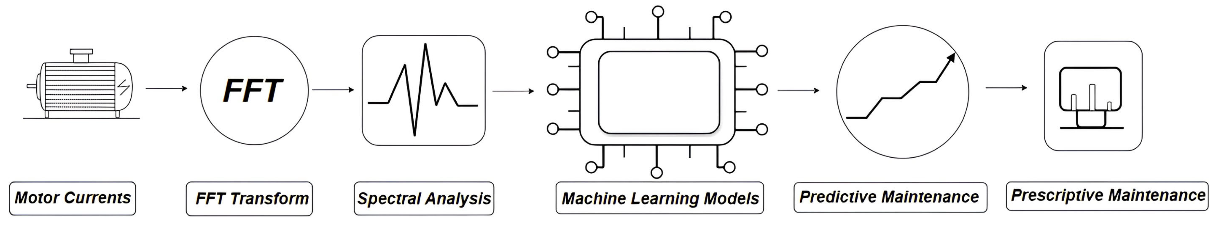
4. Advanced Machine Health Diagnosis Framework

To support the development of predictive maintenance strategies in industrial motor systems, we propose an integrated framework that combines non-invasive current monitoring with advanced signal processing and deep learning algorithms. The goal is to enable accurate fault prediction and deliver prescriptive maintenance recommendations in real time. The proposed framework is composed of six core stages, each designed to transform raw electrical data into actionable insights, as shown in Figure 2.

4.1. Current Signal Acquisition

The system begins with the continuous acquisition of motor current data from installed sensors, typically at the phase level. As this step is non-intrusive and leverages existing motor instrumentation, it ensures minimal disruption to operations while capturing dynamic electrical behavior over time.

4.2. Frequency-Domain Transformation

The acquired time-domain signals are converted into the frequency domain using the Fast Fourier Transform (FFT) [18]. This process isolates the harmonic content of the signal, revealing fault-related frequency components that may indicate early stage degradation. Frequency resolution and noise filtering are adjusted according to the application requirements.

4.3. Spectral Feature Extraction

From the transformed signals, key features are extracted, such as amplitude values at specific frequency bands, sideband patterns, and statistical descriptors. These features form the diagnostic basis for identifying anomalies and feeding machine learning models with structured, highly informative data.

4.4. Machine Learning-Based Prediction

Extracted features are then input into a trained machine learning model, with long short-term memory (LSTM) networks serving as the core prediction engine. The LSTM captures the temporal evolution of spectral patterns and forecasts future degradation behavior [19]. This step enables proactive fault anticipation rather than mere detection.

4.5. Fault Severity Assessment

The predicted degradation trend is projected onto a predefined health scale that classifies fault severity into distinct levels (e.g., incipient, moderate, critical). This classification is based on the amplitude of the fault frequency component. As the amplitude increases and crosses specific thresholds, the system assigns the fault to a corresponding severity class.

These thresholds are established either from historical data patterns or expert-defined criteria and reflect the typical progression of the fault under real operating conditions.

For example, low amplitude values indicate normal degradation (incipient), moderate amplitudes reflect a progressing fault that may soon impact performance, and high amplitudes correspond to a critical condition requiring immediate attention.

This data-driven classification supports maintenance teams by providing a clear, risk-based view of asset health, enabling the prioritization of interventions based on severity and estimated time-to-failure.

4.6. Prescriptive Maintenance Recommendation

Based on the assessed fault severity, the system generates targeted prescriptive maintenance recommendations. These actions are directly aligned with the predicted risk level and may include alerts for inspection, recommendations for component replacement, or automatic scheduling of maintenance activities within existing operational workflows. The severity assessment and all the corresponding actions are based on the amplitude of the fault frequency component.

By translating diagnostic output into actionable guidance, the prescriptive layer serves as a critical bridge between data-driven monitoring and maintenance execution. This integration enables faster, more informed decision-making, reduces unplanned downtime, and strengthens overall asset reliability and operational continuity.

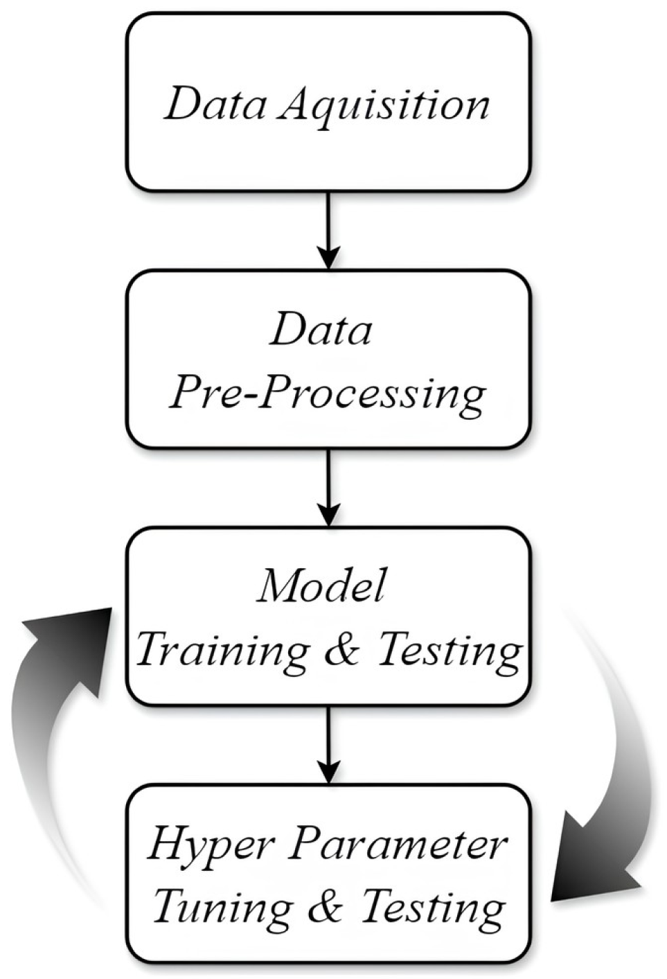
5. Methodology

This study employed a systematic methodology to verify the model’s capability and potential by testing it against real spectral component data of belt failure. Each phase of the methodology is detailed below, with Figure 3 providing an illustrative overview of the process.

5.1. Data Acquisition and Preparation

The first phase involved the acquisition of raw spectral component data of belt failure from the industrial fan monitored. This process ensured the collection of comprehensive and accurate data necessary for subsequent analysis.

Following data acquisition, the raw data underwent meticulous pre-processing to prepare them for analysis. This step involved the removal of any outliers and the application of data cleaning techniques to enhance data quality and reliability.

5.2. Model Training and Testing

The pre-processed data were then subjected to model training and testing, a crucial phase in developing the prognostic model. A machine-learning algorithm was employed to train the model using the normalized data, aiming to capture patterns and relationships that could aid in predicting belt failure.

Once the initial model was trained, hyper parameter testing and fine-tuning were conducted to optimize its performance. This iterative process involved adjusting model parameters such as learning rate, batch size, and number of hidden layers to enhance predictive accuracy and generalization capability. Following hyper parameter tuning, the model underwent rigorous evaluation and validation to assess its predictive performance. Various metrics such as RMSE, MAPE, and accuracy were used to measure the model’s effectiveness in forecasting belt failure, as described in Section 8.1.

6. Case Study

To validate the proposed framework in a real-world industrial context, a case study was conducted on an induction motor operating a belt-driven transmission system. The objective was to evaluate the framework’s effectiveness in detecting, predicting, and prescribing responses to progressive mechanical degradation, using only non-intrusive electrical measurements.

6.1. Experimental Setup

The experimental setup employed in this study features an industrial fan, as shown in Figure 4, monitored through ENGING’s online platform, which enables the continuous extraction of motor current signals and spectral components essential for belt fault detection (

Table 2. Main nominal parameters of the motor.

Power	Voltage	Current	Frequency
200 kW	400 V	346 A	50 Hz

and

Table 3. Industrial fan information.

Dmotor_pulley	fr	Lbelt
300 mm	24.83 Hz	5600 mm

).

While the framework was tested on a single asset, it was designed to be scalable and transferable. Since it uses only electrical data, it can be applied to a wide range of motors and assets with minimal adaptation. This makes it well-suited for integration across different industrial environments.

Nevertheless, scaling to multiple motors may present challenges such as variations in load, operational profiles, or motor characteristics. However, these can be addressed through model retraining or parameter tuning. The method’s modularity and data-driven nature support this flexibility.

6.2. Dataset

The dataset used in this study encompasses nearly two years of high-resolution spectral data, capturing essential electrical and mechanical dynamics of the system. Key spectral components, such as the supply frequency, the motor rotation frequency, the load-related harmonics, and the belt fault frequency, were recorded with high fidelity, at a resolution of 0.1 Hz and spanning a spectral range of up to 1250 Hz. From this rich dataset, a series of features was extracted to characterize both the signal’s magnitude and its evolution over time.

For the scope of this study, the analysis was intentionally focused on the belt fault frequency, as it represents the most direct and diagnostically relevant indicator of progressive belt degradation. This targeted approach enabled the precise assessment of the spectral behavior associated with the fault condition, improving interpretability and ensuring that the model addresses a specific, high-impact failure mode.

To evaluate model performance, the dataset was split into training (80%) and testing (20%) sets using a strict chronological division. All training data preceded the test set in time, ensuring full preservation of temporal order and preventing any future information from leaking into the training process. This time-aware split was carefully chosen to reflect real-world predictive maintenance use cases, where historical data were used to forecast future asset behavior.

Although more rigorous validation strategies, such as walk-forward or roll-window validation, could further enhance robustness, the chosen approach strikes a practical balance between methodological rigor and computational feasibility. Given the long time span, the quality of the data, and the naturally occurring degradation patterns captured, the adopted split provides a representative and reliable basis for evaluating model generalization.

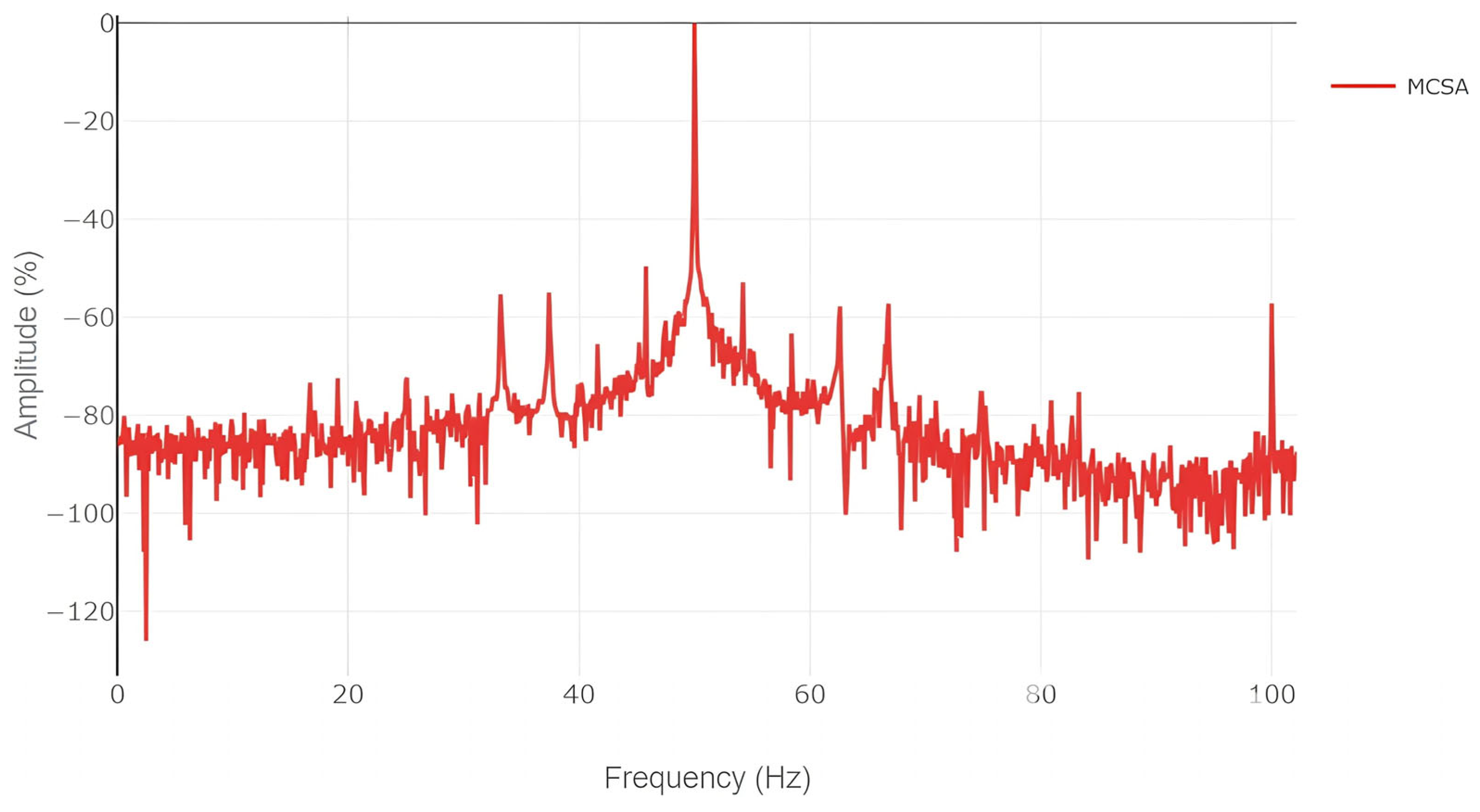
6.3. Data Analysis

An initial visual inspection of the spectral data indicated the presence of a recurring component near 4.2 Hz, later identified as a characteristic frequency related to belt vibration. This frequency was calculated based on the known geometry and speed of the transmission system, and its amplitude was monitored over time as a degradation indicator.

Belt Failure

The first step in monitoring the frequency components of the belt characteristics is to calculate the frequency of the belt (f_b) [32]. In this case, f_b is the characteristic frequency of the belt given by the following:

$$f_b={\displaystyle \frac{\left(D_{\mathit{motor}\text{\_}\mathit{pulley}}\cdot \pi \cdot f_r\right)}{L_{\mathit{belt}}}}$$

(4)

where f_r is the rotation frequency, D_{motor_pulley} is the diameter of the motor pulley, and L_belt is the length of the belt. The sideband components of the fundamental are 323 at f₁ ± f_b.

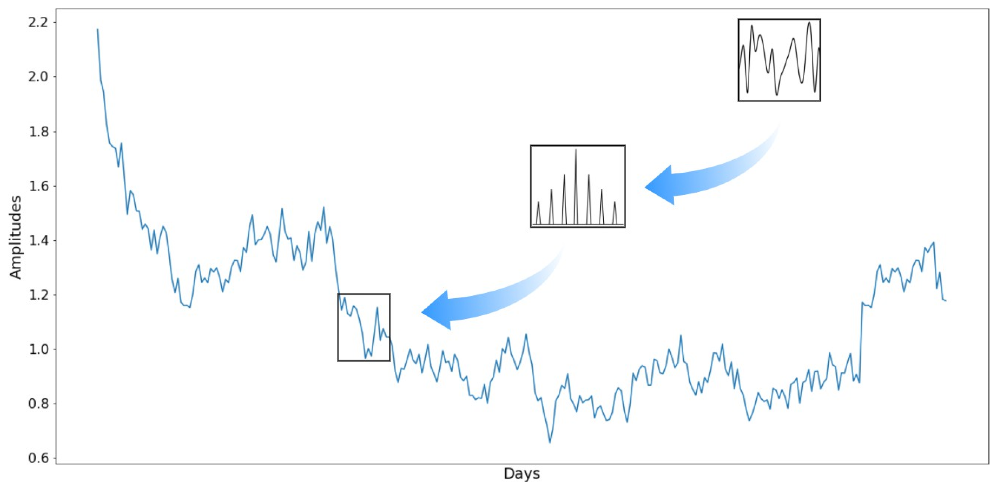
To reduce noise and dimensionality, the dataset was filtered to isolate amplitude values corresponding to frequencies between 4.1 and 4.3 Hz. Outliers due to load variation or unrelated mechanical anomalies (e.g., eccentricity near 24.5 Hz) were removed to ensure data consistency. As seen in Figure 5, when the asset is operating with issues, there is significant noise across the spectrum, with the frequency of the belts exhibiting the highest amplitude.

In Figure 6, it is possible to see a scheme illustrating the data transformation process leading to the obtained curve of the belt failure over time.

7. Prediction Models

Since belt failure records can be considered as a multivariate time series and the current state of a particular failure is expected to be related to previous states, two models were considered for this study.

Initially, the ARIMA (AutoRegressive Integrated Moving Average) model was considered due to its widespread application in time series forecasting [10,11]. ARIMA is particularly effective for modeling univariate time series that exhibit non-stationary behavior, which can be addressed through differencing techniques [33]. The model comprises the following three key components: an autoregressive (AR) part that captures the influence of past values, an integrated (I) part that accounts for the level of differencing required to achieve stationarity, and a moving average (MA) part that models the impact of past forecast errors. These are denoted by the parameters p, d, and q, respectively. When non-stationarity is detected in the data, differencing is applied to stabilize the mean and remove trends, thus transforming the series into a stationary form suitable for further analysis [34].

Subsequently, a deep learning model was considered, particularly an LSTM model [12,13,35]. A sequence of two years of failure component records was used to predict its future evolution.

The values of the hyperparameters were experimentally optimized.

Table 4. Characteristics of the ARIMA model.

Model	p	d	q
ARIMA	3	1	2

and

Table 5. Characteristics of the LSTM model.

Model	LSTM-Sigmoid	LSTM-Tanh	LSTM-ReLU
No. of Hidden Layers	1	1	1
No. of Memory Units	35	40	35
Optimizer	ADAM	SGD	ADAMAX
Batch Size	2	2	2
No. of Epochs	100	100	100

present the parameters used for each model.

For both the LSTM and ARIMA models, they utilized a time series of input data representing the historical performance of the belt system. Each data point in the time series represents a specific measurement of the belt failure frequency over time. The goal of both models was to predict the future performance of the electric motor based on the input data.

For ARIMA, a series of iterations was conducted to discover the optimal values of p, d, and q, and the autocorrelation plots and model diagnostic tests were performed to ensure that the model was well-constructed. Similarly, for LSTM, the same process was carried out, starting with its parameterization and various tests on the correct percentage division into training and testing data until reaching the parameterization described above.

In summary, both the LSTM and ARIMA models underwent rigorous testing and parameter optimization to ensure accurate predictions of the electric motor’s performance. The details of these experiments and the results obtained are discussed in the following sections.

8. Experiments and Results

In this section, the experiments conducted and the results obtained when applying the LSTM model for predicting belt failure are presented. Firstly, the specifics of the experiments conducted were outlined, followed by an analysis of the results and their interpretation.

8.1. Performance Metrics

Assessments of the models used in this work were based on root mean squared error (RMSE), mean average percentage error (MAPE), and accuracy. The formula for calculating RMSE is expressed in Equation (5):

$$RMSE=\sqrt{{\displaystyle \frac{1}{n}}\sum _{i=1}^n{\left(y_i-{\hat{y}}_i\right)}^2}$$

(5)

• n is the total number of observations in the test sample;
• y_i represents the actual value at position i;
• ${\hat{y}}_i$ represents the predicted value at position i.

The RMSE is useful because it provides a measure of error that is in the same unit as the original data, thus facilitating direct interpretation. The lower the RMSE value, the better the model performance, indicating a closer agreement between the predicted values and the actual values [31].

The calculation of MAPE is straightforward and intuitive. For each data point in the test sample, by calculating the absolute percentage difference between the predicted value and the actual value, the average of these differences is obtained [36]. The formula for calculating MAPE is given by the following:

$$MAPE={\displaystyle \frac{1}{n}}\times \sum _{i=1}^n\left|{\displaystyle \frac{y_i-{\widehat{y}}_i}{y_i}}\right|\times 100\%$$

(6)

where:

• n is the total number of observations in the test sample;
• y_i represents the actual value at position i;
• ${\hat{y}}_i$ represents the predicted value at position i.

Finally, accuracy is a fundamental metric for evaluating the overall quality of prediction models [37]. Mathematically, accuracy is calculated as follows:

$$\mathit{Accuracy}={\displaystyle \frac{TP+TN}{n}}\times 100\mathrm{\%}$$

(7)

where:

• TP is the number of correct predictions for samples in the class;
• TN is the number of correct predictions for samples out of the class;
• n is the total number of observations in the test sample.

A high accuracy indicates that the model is making accurate predictions and is correct most of the time, while a low accuracy suggests that the model is struggling to predict observations correctly.

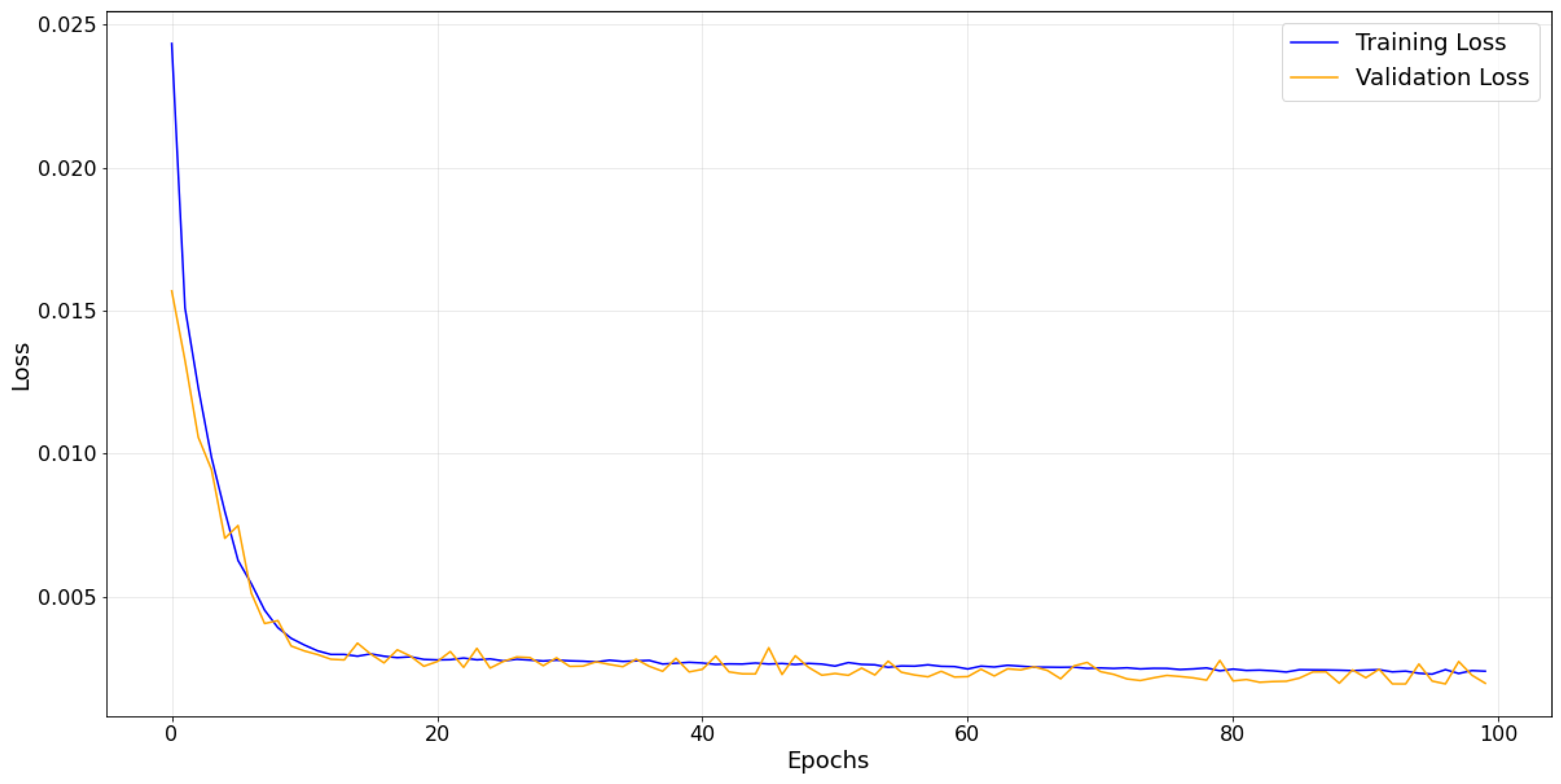
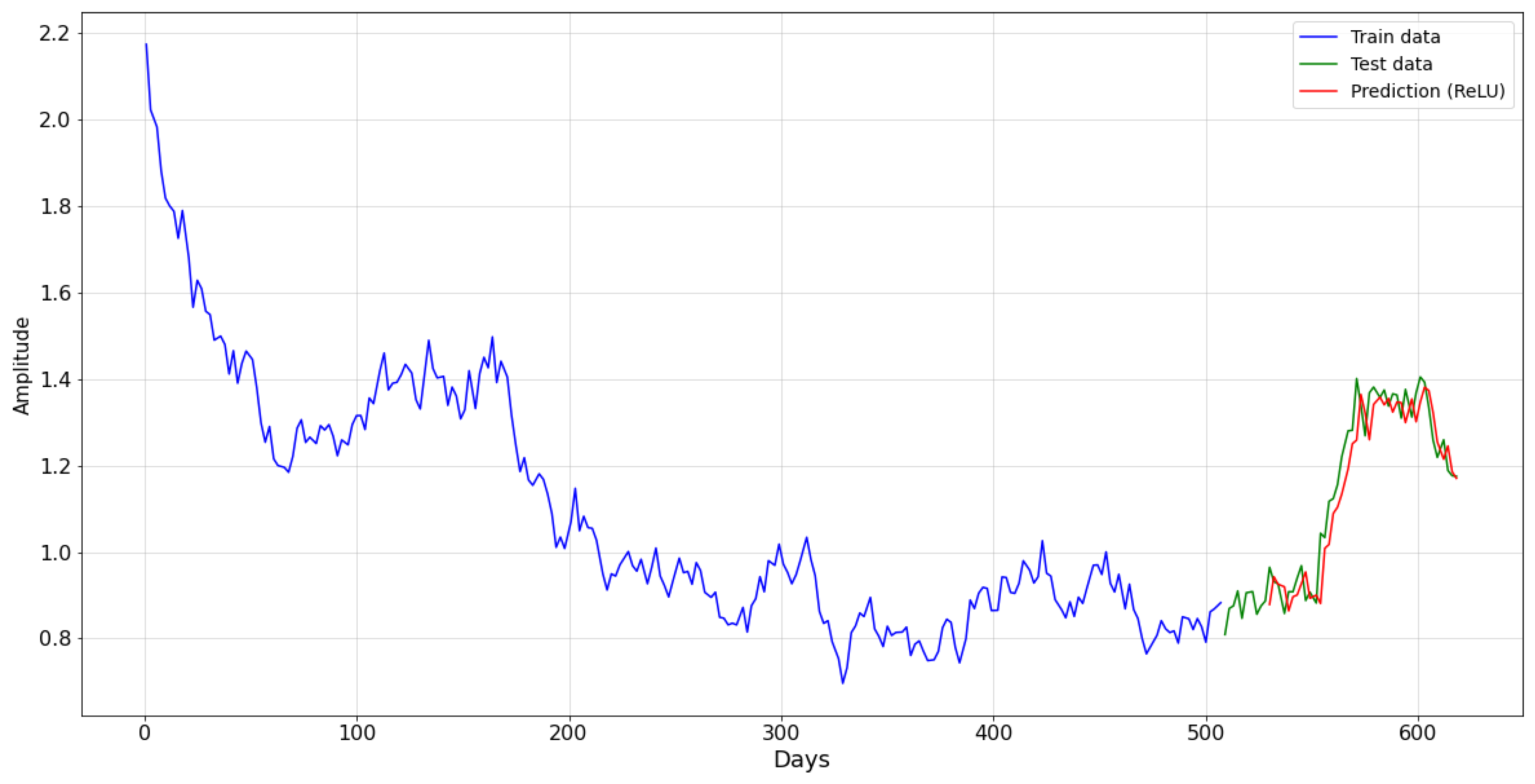
LSTM-ReLU

The performance of the LSTM—ReLU model was the one that showed the best results, as can be seen in Figure 7 and Figure 8.

Figure 8 shows the graph of the predicted and actual amplitude values of the belt failure component. The green color represents the actual amplitudes of the belt failure component, while the red color represents the predicted values. The proposed model accurately predicted the normal values and followed the degradation trend, which was also efficiently predicted.

8.2. Results Comparison

The results achieved by the LSTM—ReLU model and all other tested models are presented in

Table 6. Model evaluation using various metrics.

Model	RMSE	MAPE	Accuracy
ARIMA	0.1	11.20%	88.8%
LSTM-Sigmoid	0.07	6.40%	92.30%
LSTM-Tanh	0.09	7.80%	91.70%
LSTM-ReLu	0.05	5.20%	94.80%

, along with their respective performance comparisons.

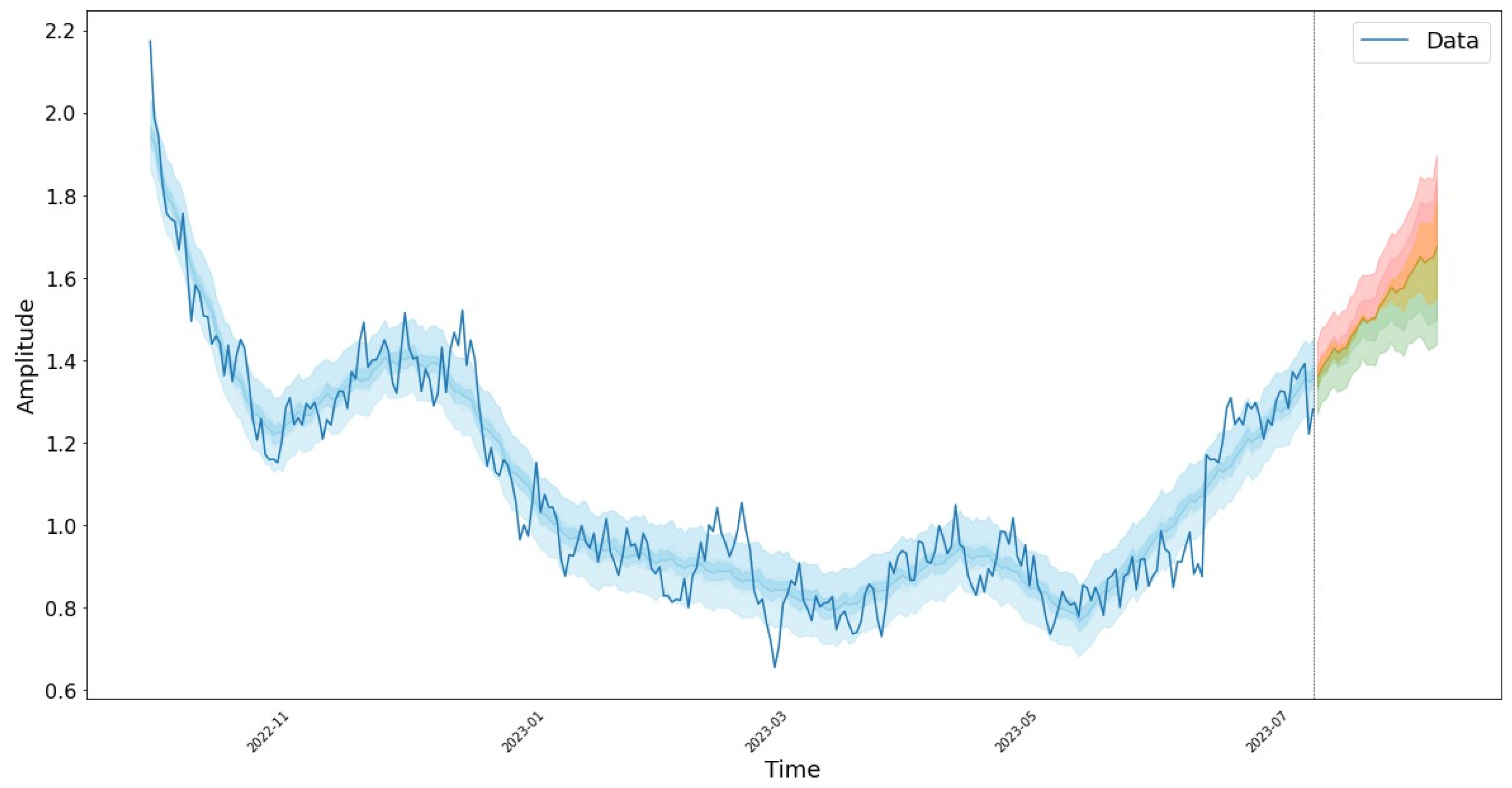
In addition, a forward-looking forecast was generated, predicting the next days based on the previous data. Multiple scenarios were illustrated, as depicted in Figure 9, including optimistic and pessimistic fault trajectories, providing a comprehensive view of potential outcomes.

8.3. Fault-Oriented Prescription

To enhance interpretability and support maintenance decision-making, the predicted amplitude values of the fault frequency component were mapped onto a three-tier risk scale that included green, yellow, and red zones. This health classification scheme enables the intuitive visualization of the asset’s condition and helps prioritize interventions.

• GreenZone: This zone corresponds to low-amplitude variations within the expected operating range. When the predicted values remain within this region, the belt system is considered to be in stable condition, with no indication of significant wear or misalignment. In this scenario, no immediate action is required beyond regular monitoring.
• YellowZone: As the predicted amplitude begins to enter this intermediate zone, it indicates an accelerated degradation trend. This suggests the emergence of wear or tension irregularities in the belt system. Although the asset remains operational, it is recommended that the maintenance team prepares for further inspection, as the likelihood of progression toward failure increases.
• RedZone: This level reflects a critical condition in which the amplitude of the fault frequency is significantly elevated. It signals that a failure is likely under development and that immediate action is required. The system automatically recommends an inspection of the transmission mechanism, with particular focus on verifying belt tension, pulley alignment, and possible belt replacement if necessary.

Importantly, the thresholds used are not generic but are personalized for each asset, which is key to the system’s real value. Generic thresholds could lead to many false positives or false negatives, reducing reliability. However, this tool is not a plug-and-play solution, it requires a learning period, approximately 15 days in this study, during which the model learns the asset’s normal behavior to adjust and fine-tune the thresholds.

Although this process is not fully automatic, the learning phase is essential to capture the typical operational profile of the asset. This allows the system to set accurate limits, minimizing false alarms and providing meaningful insights to maintenance teams and asset managers, tailored to the specific operating conditions.

This zone-based prescription mechanism not only aids in the interpretation of predictive results, but it also shifts maintenance from predictive to prescriptive. By linking specific actions to each risk level, the system transforms passive condition monitoring into an intelligent decision-oriented process and proactively recommends targeted interventions based on the expected progression of the fault, enabling teams to act before failures occur, improving operational continuity, reducing unplanned downtime, and optimizing asset life-cycle management.

9. Conclusions

This work introduces and validates a robust, scalable, and non-intrusive framework for predicting belt degradation in induction motor-driven systems by combining motor current signature analysis (MCSA) with advanced deep learning models. By employing LSTM networks, particularly the LSTM-ReLU variant with spectral analysis, the framework effectively captures the evolving patterns of hidden faults over time with both accuracy and interpretability.

Extensive testing on a long-term industrial dataset demonstrates that this approach consistently outperforms traditional methods such as ARIMA, while also providing a prescriptive layer that supports maintenance decisions with clear and actionable insights. This ability to convert electrical signals into reliable prognostic information promotes proactive maintenance, helping to avoid unexpected failures and reduce downtime.

That said, analysis using higher-resolution data and multi-band spectral features could potentially reveal additional insights and influence model performance. However, since this study was developed in close collaboration with an industrial partner, practical considerations require balancing the maximum achievable resolution with computational efficiency and user interpretability. The current focus on a well-defined fault frequency has yielded strong predictive results, suggesting that while incorporating multi-band analysis and finer resolution might enhance the model, these improvements are unlikely to deliver significant additional value for the main end users, maintenance teams, and asset managers. In other words, the current approach optimizes the trade-off between detailed data analysis and operational usefulness, ensuring that the framework remains both effective and accessible. Overall, this research offers not only a highly accurate fault prediction model but also a practical decision support tool aligned with Industry 4.0 objectives, enhancing operational reliability, extending asset lifespan, and maximizing the benefits of data-driven maintenance strategies. Furthermore, the proposed methodology can be readily integrated with other Industry 4.0 technologies to create more comprehensive and intelligent maintenance systems. For example, it can leverage IoT sensors to collect diverse real-time data streams from multiple assets, enhancing the granularity and the scope of monitoring. Cloud computing and edge processing can support scalable data storage and rapid model inference, enabling near real-time fault detection and response. In addition, combining this framework with advanced analytics and digital twin technologies can facilitate predictive simulations and scenario planning, further optimizing maintenance scheduling and asset management. This integration ensures that the methodology is not only effective in isolation but is also adaptable to evolving smart factory environments, supporting more automated, flexible, and efficient industrial operations.

10. Future Work

This study provides a validated framework for predictive maintenance using electrical signals and deep learning, but it does not implement domain adaptation or transfer learning strategies. However, these approaches were discussed and are considered highly relevant for future developments, particularly in the context of scaling the framework across different industrial settings or motor types.

Future research should explore domain-adaptation techniques to improve the model’s ability to handle data from different operating conditions, motor specifications, or industrial environments. By aligning feature distributions between source and target domains, these methods could reduce performance degradation when the framework is applied to new assets or plants without requiring full model retraining.

Similarly, transfer learning presents a valuable opportunity to reuse knowledge learned from one asset such as a specific motor and apply it to another with minimal labeled data. This is especially relevant given the framework’s design, which is modular and generalizable. It could be adapted to various types of rotating machinery, enabling faster deployment in real-world applications with lower data and computational requirements.

In parallel, by extending the framework to incorporate multi-sensor data, including vibration and temperature would allow for a more comprehensive view of equipment health, potentially capturing fault signatures that are not evident in electrical signals alone. Reinforcement learning also remains a promising path, offering the ability to optimize maintenance policies based on continuous feedback from the environment.

Finally, these future enhancements aim to evolve the current solution into a fully adaptive, cross-domain, and intelligent maintenance framework that meets the practical challenges of diverse Industry 4.0 ecosystems.