
Welding Image Data Augmentation Method Based on LRGAN Model


Abstract
:1. Introduction
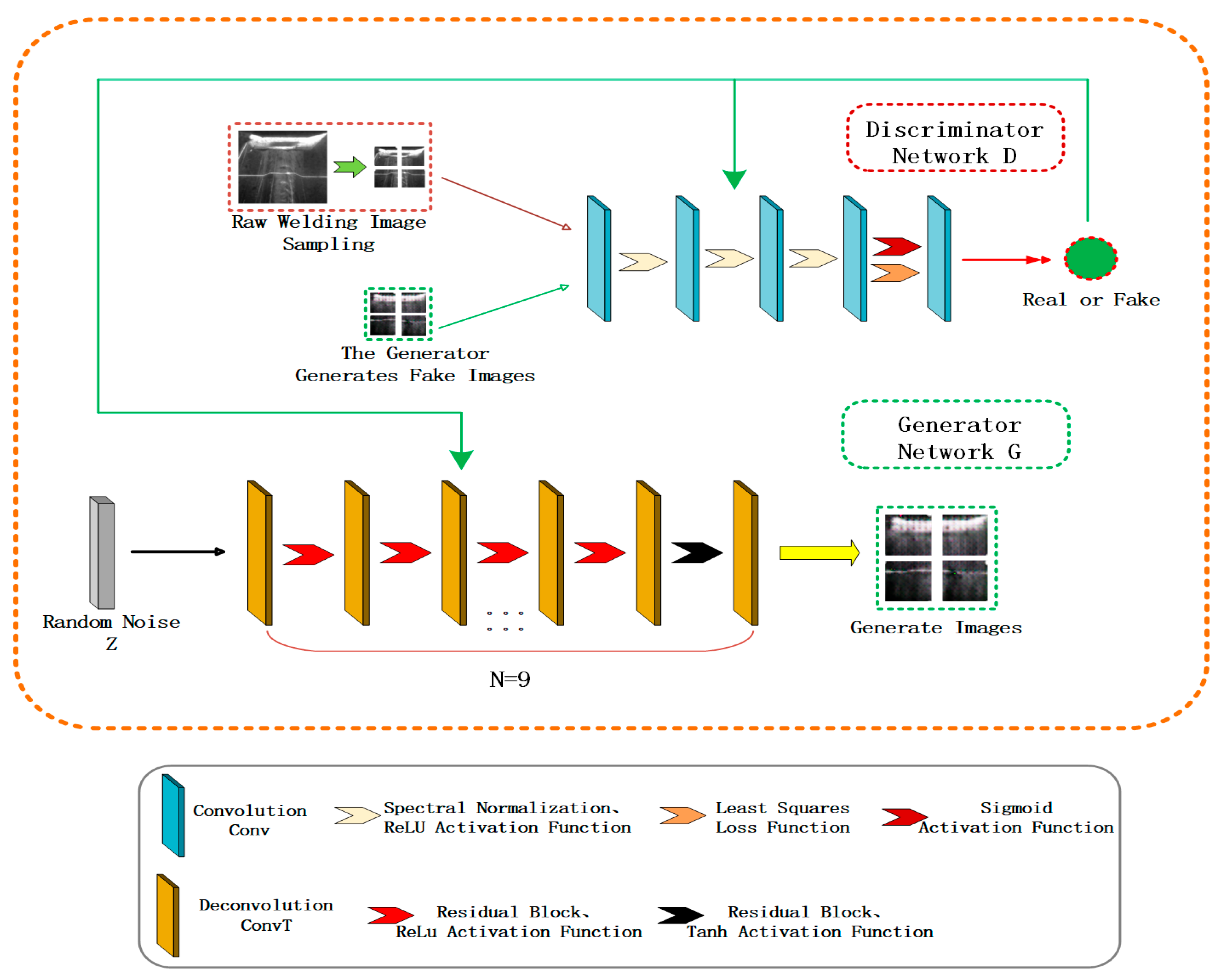
2. LRGAN Model
2.1. The Discriminator Part of the LRGAN Model
2.1.1. The Discriminator Structure of the LRGAN Model
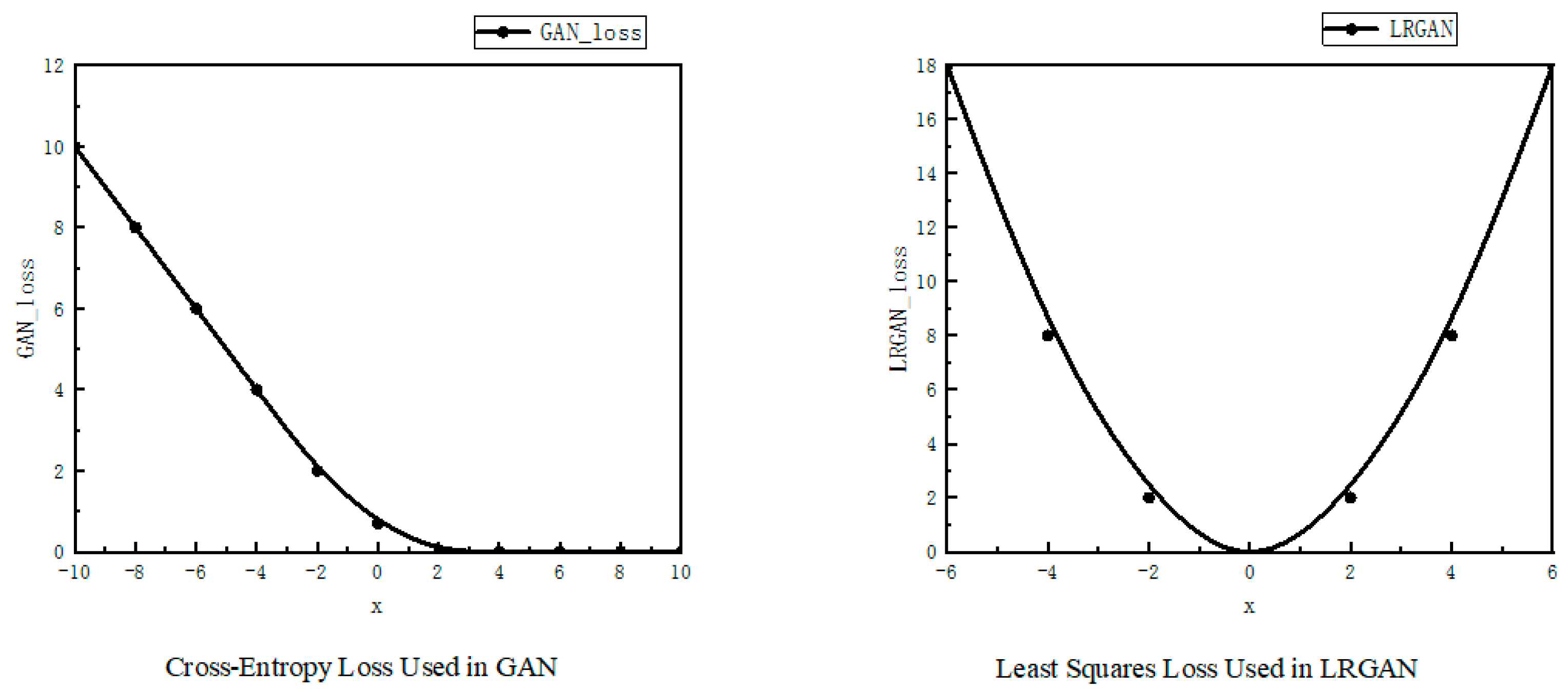
2.1.2. Loss Function
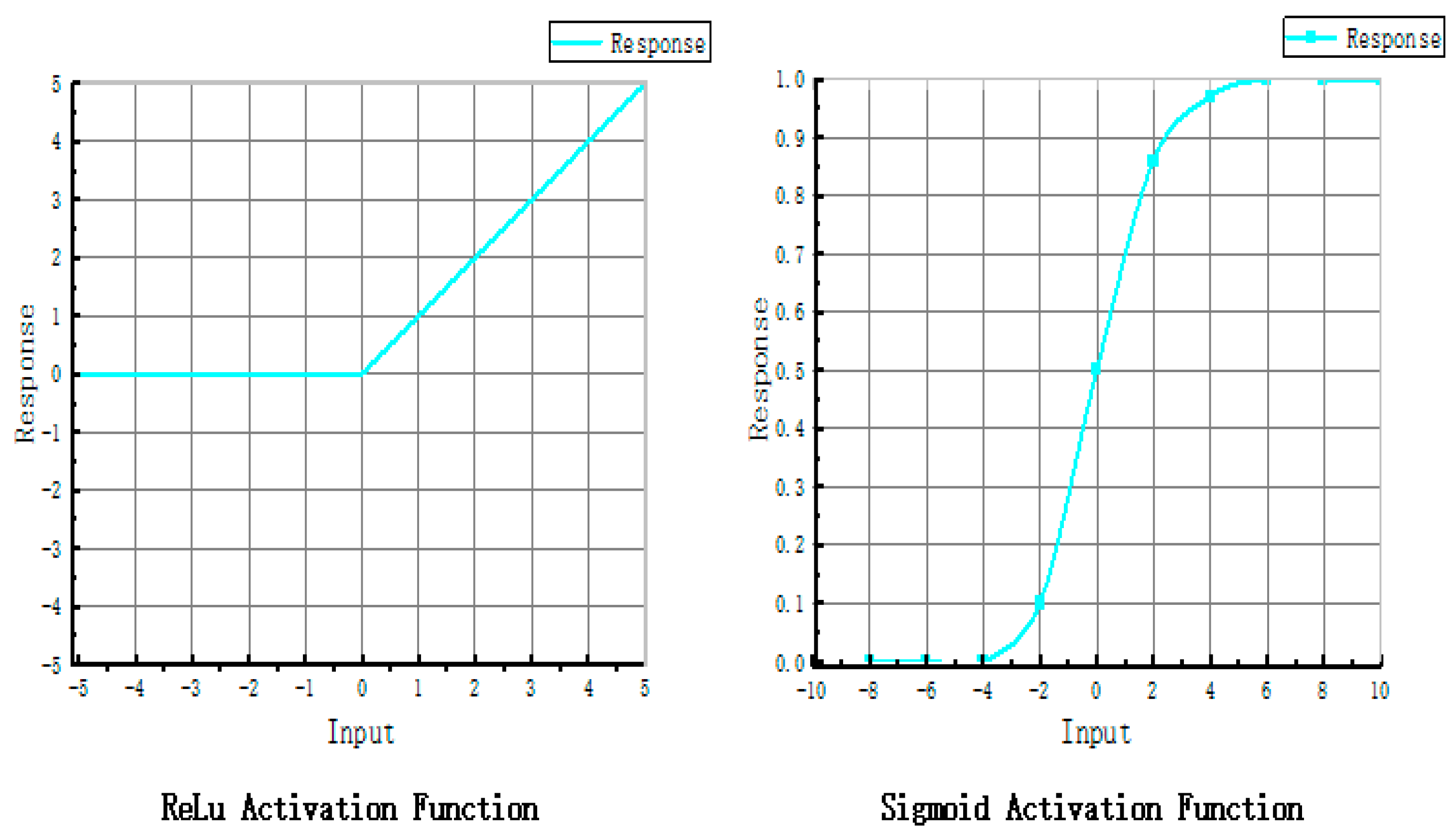
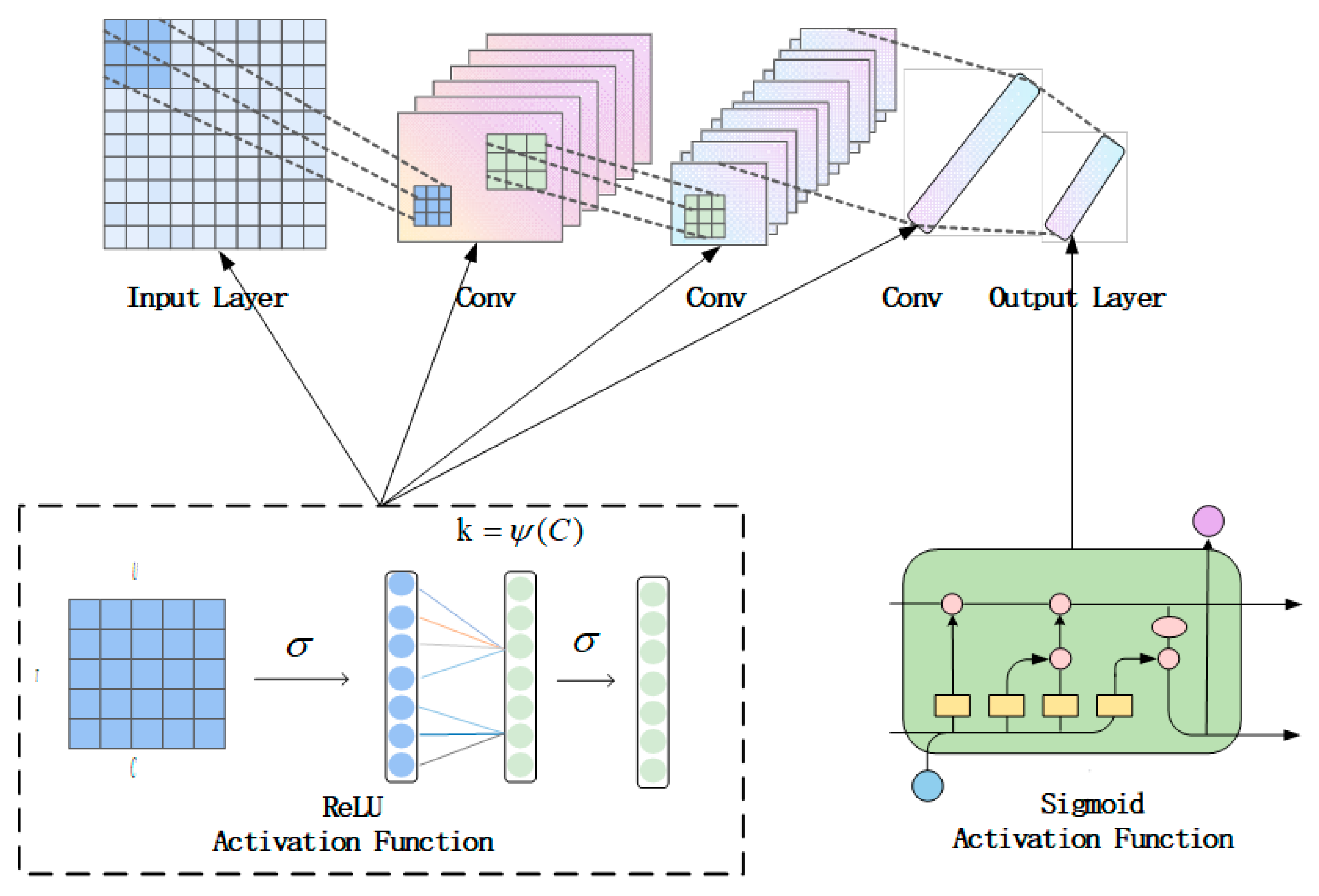
2.1.3. The Activation Function in the Discriminator
2.1.4. Spectral Normalization and Lipschitz Constant
2.2. The Generator Part of the LRGAN Model
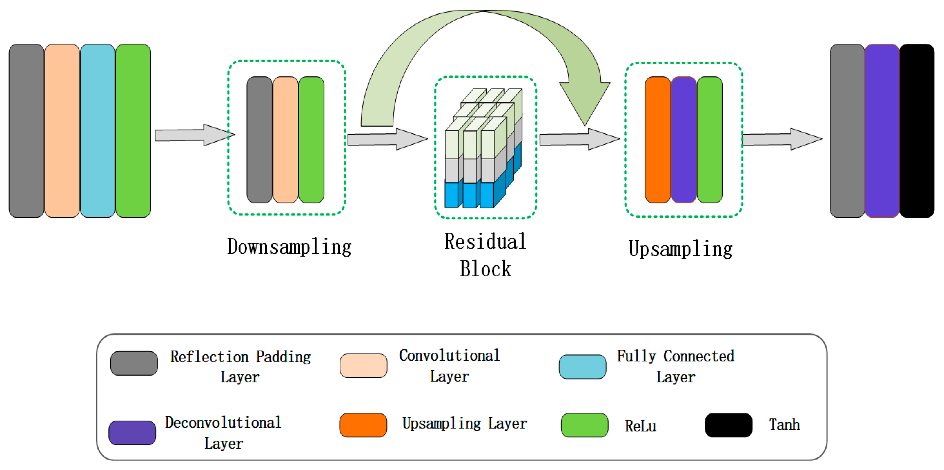
2.2.1. The Generator Structure of the LRGAN Model
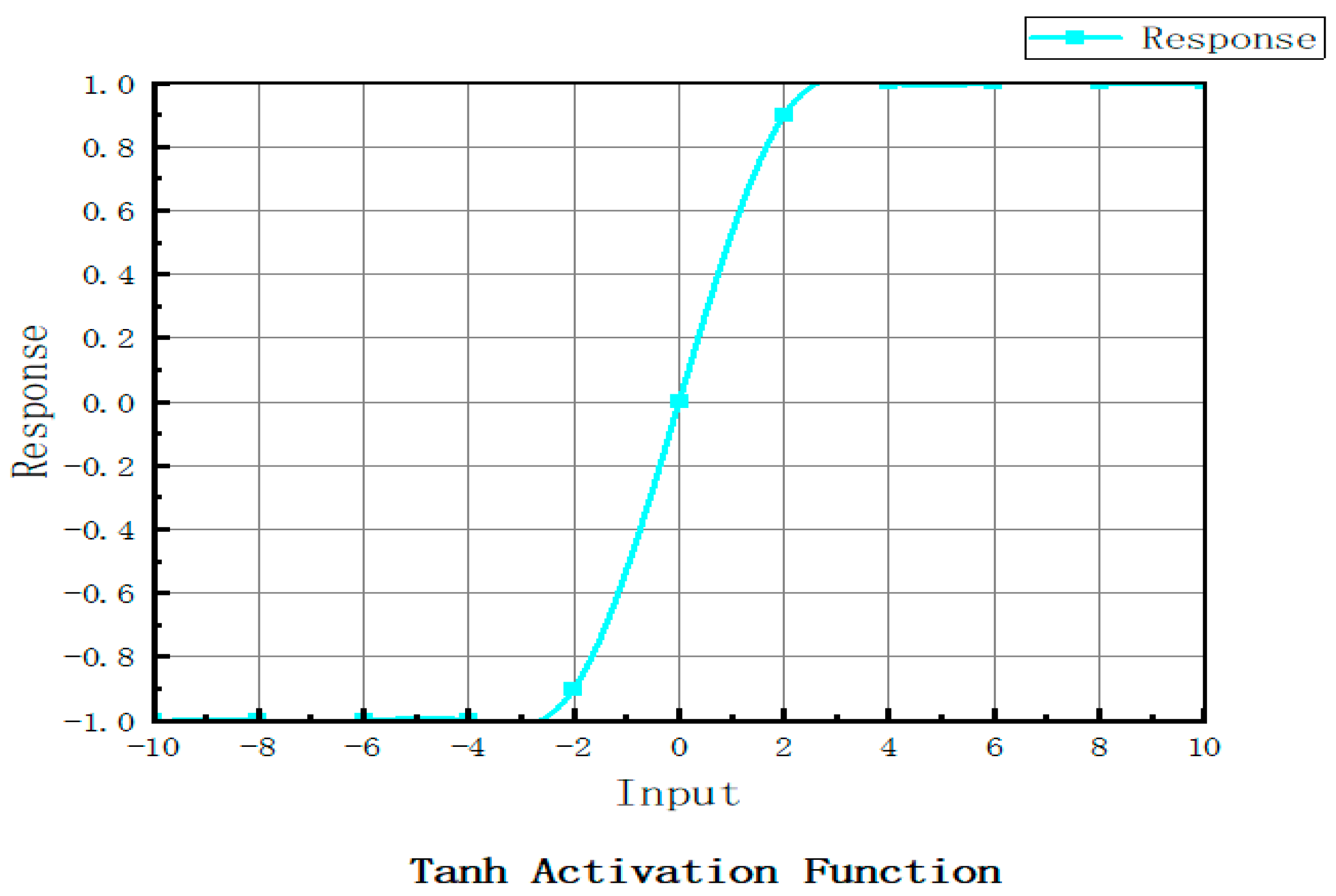
2.2.2. Generator Activation Functions
2.2.3. Nine-Layer Residual Network
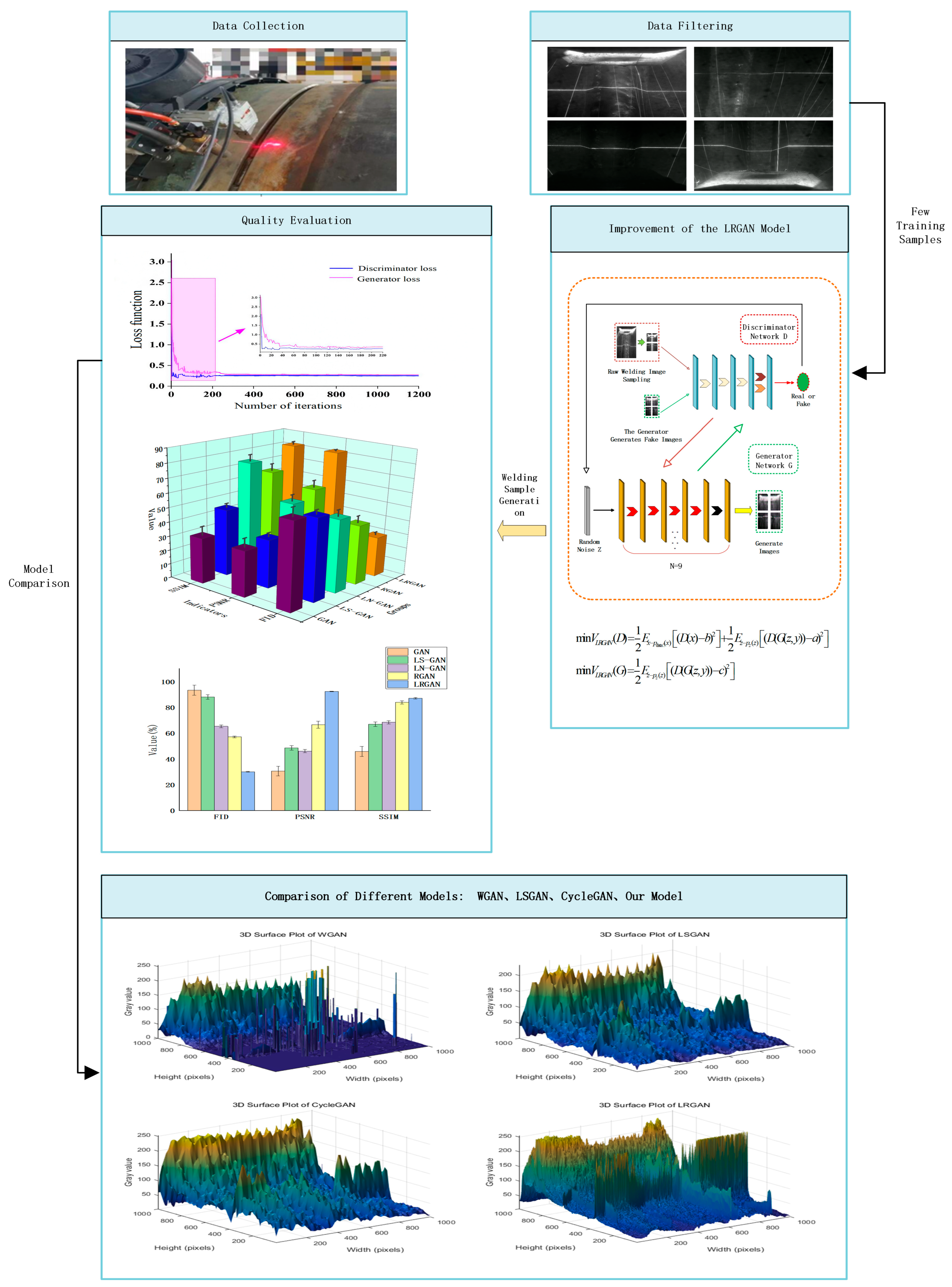
3. Experimental Process
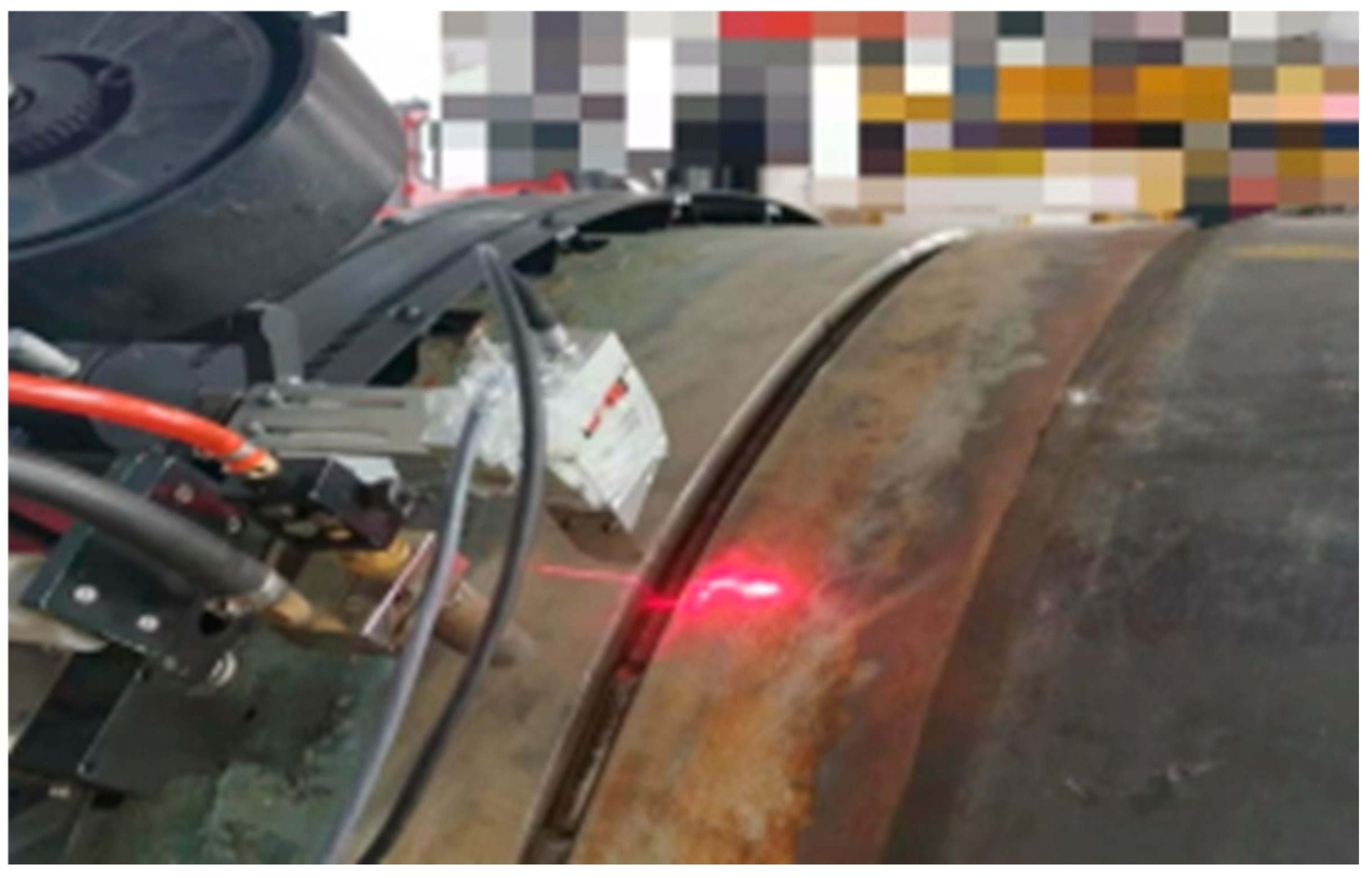
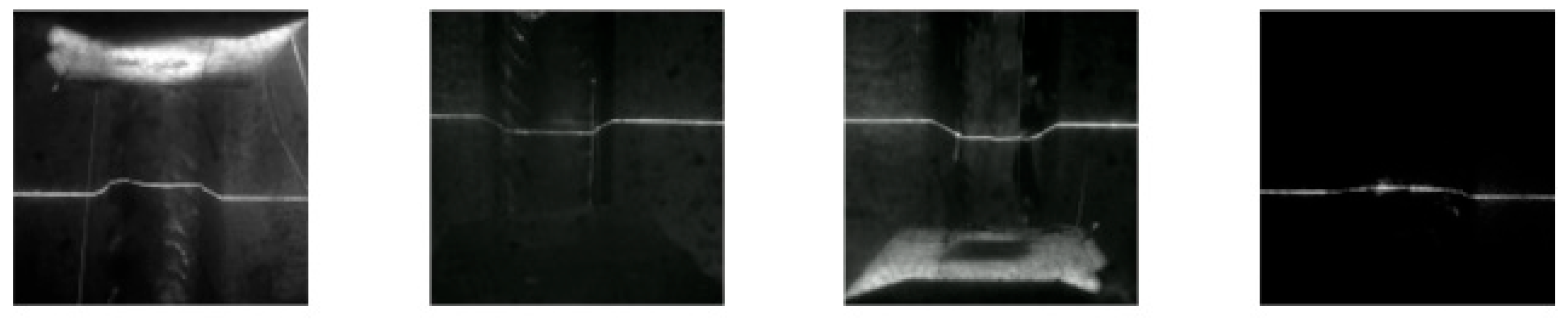
3.1. Data Preparation and Experimental Procedures
3.2. Experimental Environment
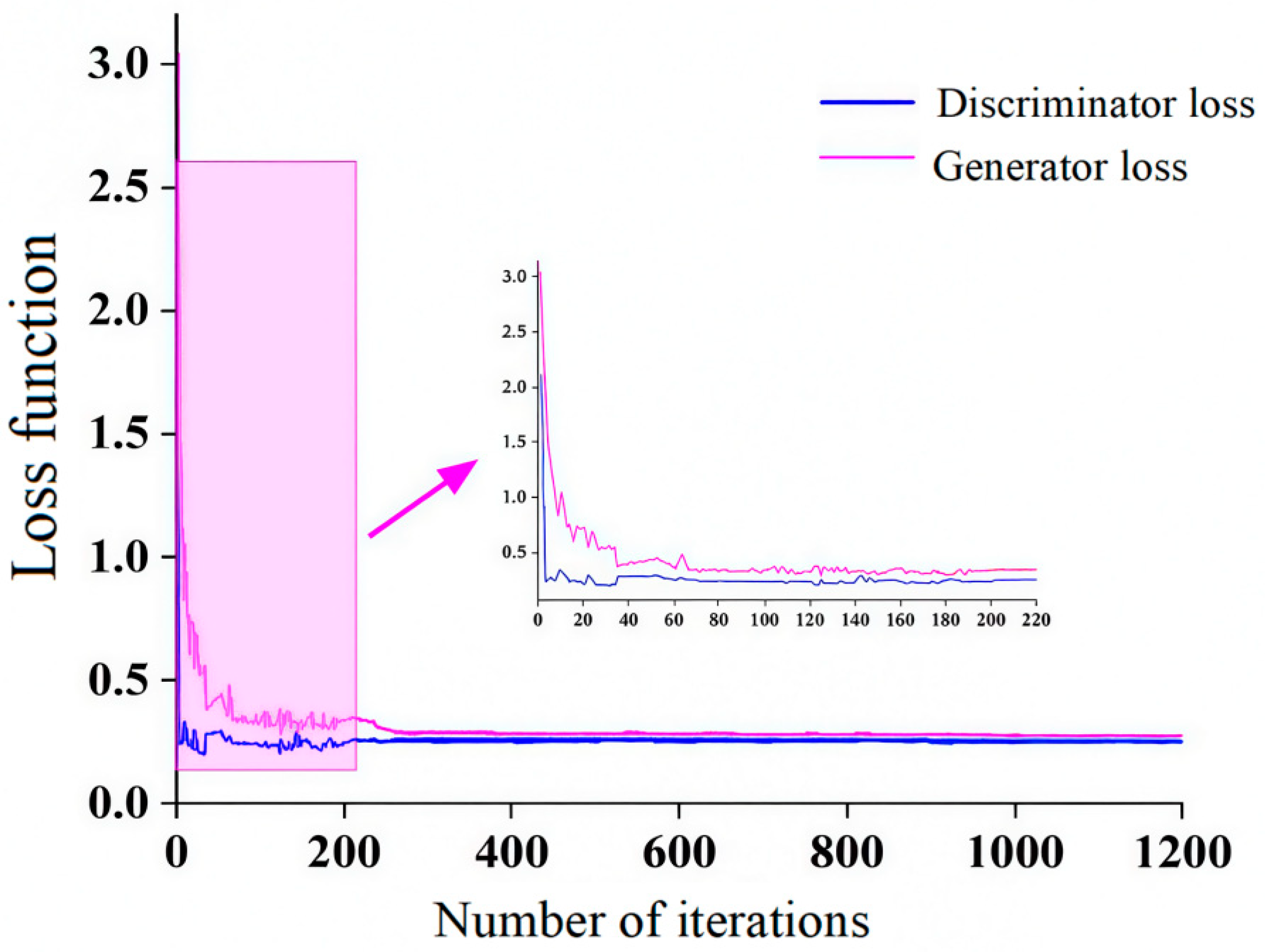
3.3. LRGAN Model Training
3.4. Generate Image Evaluation Metrics
4. Experimental Results and Discussion
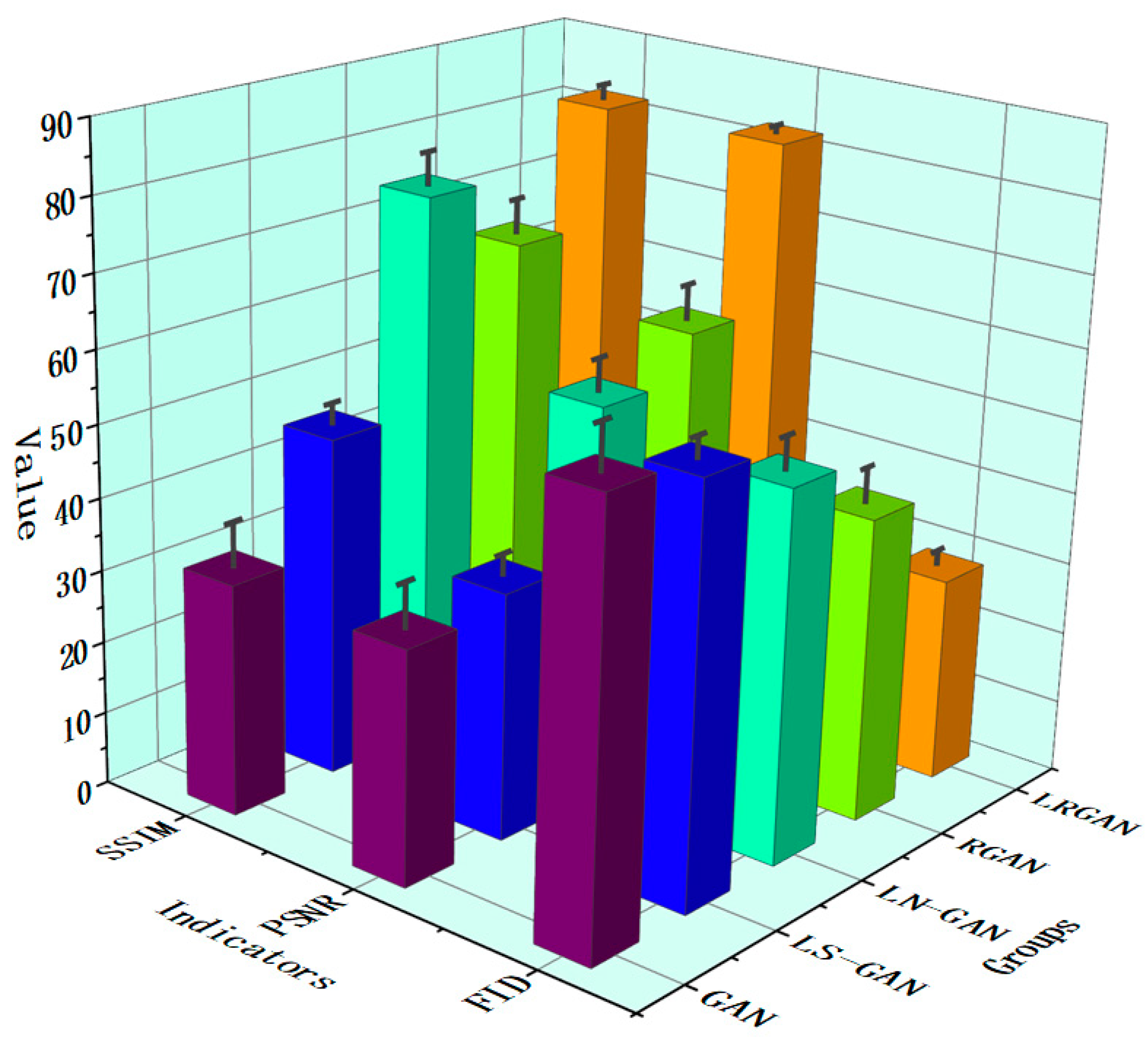
4.1. Ablation Experiment
4.2. Comparison of Images Generated by Different Models
4.2.1. Subjective Evaluation of the Results
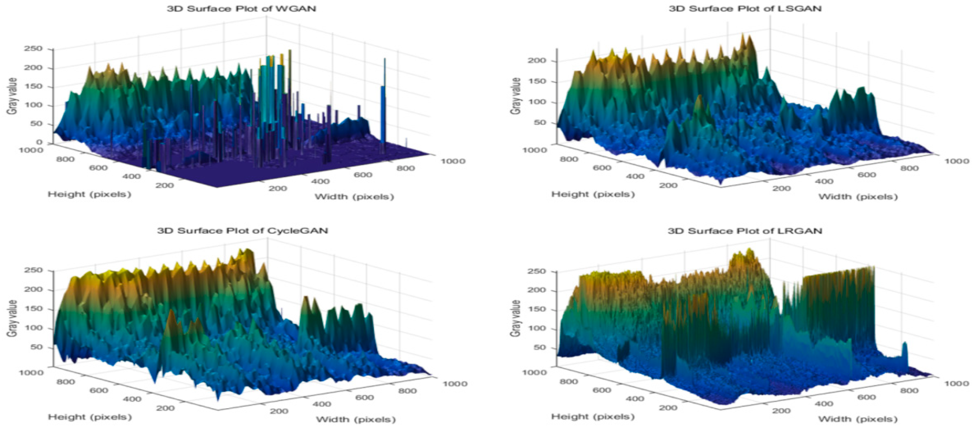
4.2.2. Grayscale 3D Surface Analysis
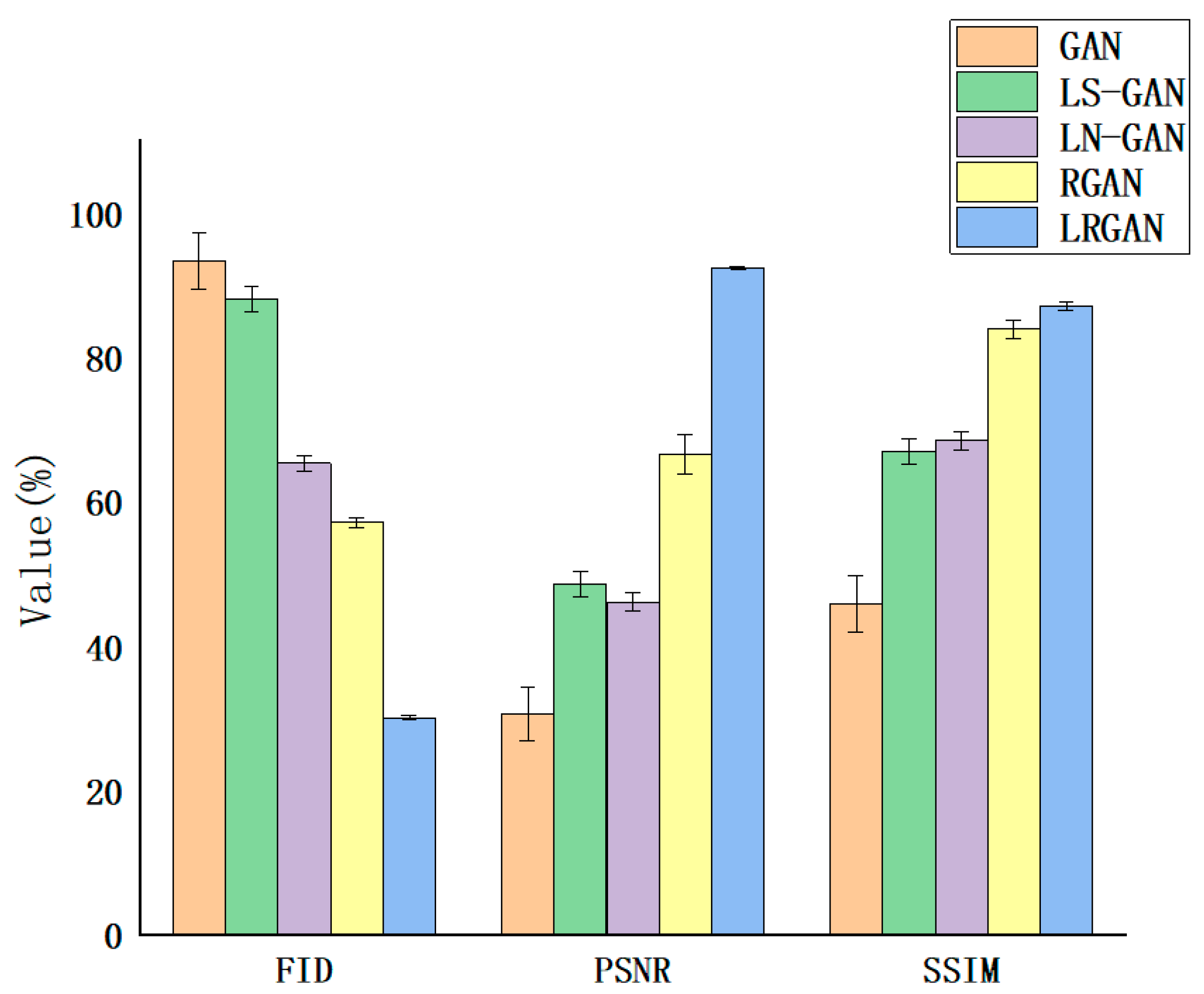
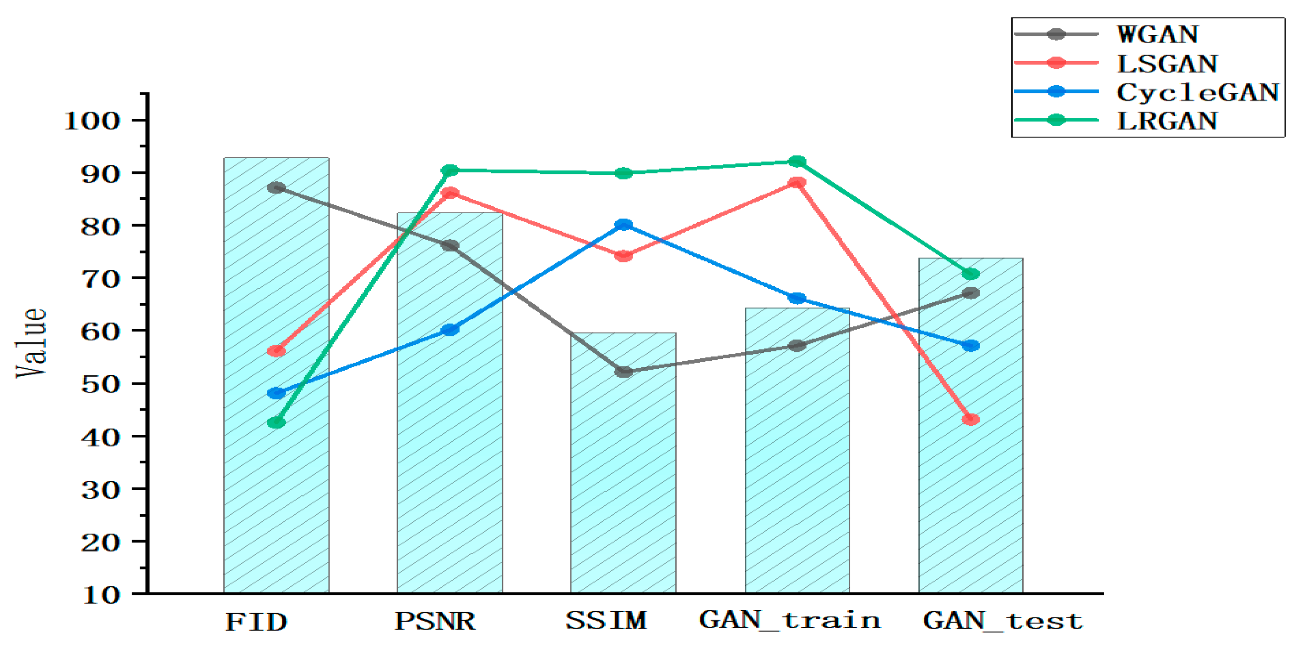
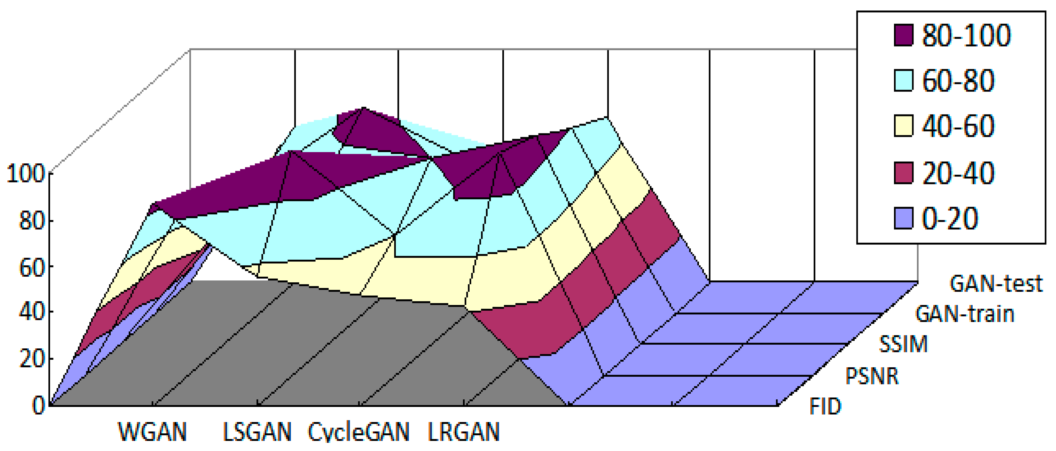
4.2.3. Quantitative Analysis
4.3. The Optimal Number of Samples for LRGAN in Few-Shot Learning
5. Conclusions
- (1)
- The least squares loss function is used to replace the original cross-entropy loss function, leading to a more stable training process. The discriminator becomes stricter and more precise in classification, making the generated images from the generator more closely resemble the original images in terms of structure and details. The least squares loss function contributes the most to controlling the SSIM and bringing its value closer to 1.
- (2)
- Spectral normalization has a more significant effect on improving PSNR. By constraining the discriminator’s Lipschitz continuity, it increases the PSNR value and enhances the model’s ability to capture the overall clarity of the image.
- (3)
- The residual structure is more helpful in reducing the FID value. It helps retain the complex texture structures of the image and reduces mode collapse.
- (4)
- The number of real data samples directly impacts the quality of the data generated by the LRGAN model. Comparative experiments with different quantities of real samples show that when the number of real data is 300, the LRGAN model achieves optimal overall performance, and the SSIM value is closer to 1. This indicates that, under this data quantity, the LRGAN model performs optimally and demonstrates good adaptability and generalization ability for small sample sizes.
- (1)
- Explore more lightweight network architectures to balance performance and deployment efficiency.
- (2)
- Introduce self-supervised learning or contrastive learning mechanisms to further enhance the model’s learning ability under ultra-small sample conditions.
- (3)
- Extend this method to the generation of multi-modal or 3D welding data to meet a broader range of industrial needs.
Author Contributions
Funding
Institutional Review Board Statement
Informed Consent Statement
Data Availability Statement
Conflicts of Interest
References
- Liu, G. Welding Quality Inspection and Management of Low-Temperature Pressure Vessels. Pop. Stand. 2024, 14, 25–27. [Google Scholar]
- Zhou, X.; Zhao, K.; Liu, J.; Chen, C. Quality Detection of Short-Cycle Arc Stud Welding Based on Deep Learning. Mod. Manuf. Eng. 2025, 1, 87–93. [Google Scholar] [CrossRef]
- Qu, J. Research on Welding Defect Detection of New Energy Vehicles Based on Improved Generative Adversarial Networks. Weld. Technol. 2024, 53, 120–125. [Google Scholar] [CrossRef]
- Goodfellow, I.; Pouget-Abadie, J.; Mirza, M.; Xu, B.; Warde-Farley, D.; Ozair, S.; Courville, A.; Bengio, Y. Generative adversarial nets. Commun. ACM 2020, 63, 139–144. [Google Scholar]
- He, Y.; Zhou, X.; Jin, J.; Song, T. PE-CycleGAN network based CBCT-sCT generation for nasopharyngeal carsinoma adaptive radiotherapy. J. South. Med. Univ. 2025, 45, 179–186. [Google Scholar] [CrossRef] [PubMed] [PubMed Central]
- Du, H.; Yuan, X.; Liu, X.; Zhu, L. Generative adversarial network image restoration algorithm based on diffusion process. J. Nanjing Univ. Inf. Sci. Technol. 2024, 1–11. [Google Scholar] [CrossRef]
- Hu, M.; Luo, C. Bearing Fault Diagnosis Based on MCNN-LSTM and Cross-Entropy Loss Function. Manuf. Technol. Mach. Tools 2024, 9, 16–22. [Google Scholar] [CrossRef]
- Liang, X.; Xing, H.; Gu, W.; Hou, T.; Ni, Z.; Wang, X. Hybrid Gaussian Network Intrusion Detection Method Based on CGAN and E-GraphSAGE. Instrumentation 2024, 11, 24–35. [Google Scholar] [CrossRef]
- Kang, M.; Shim, W.J.; Cho, M.; Park, J. Rebooting ACGAN: Auxiliary classifier GANs with stable training. Adv. Neural Inf. Process. Syst. 2021, 34, 1–13. [Google Scholar]
- Mirza, M.; Osindero, S. Conditional generative adversarial nets. arXiv 2014, arXiv:1411.1784. [Google Scholar]
- Choi, Y.; Uh, Y.J.; Yoo, J.; Ha, J.-W. StarGAN v2:diverse image synthesis for multiple domains. In Proceedings of the IEEE/CVF Conference on Computer Vision and Pattern Recognition, Seattle, WA, USA, 14–19 June 2020; pp. 8188–8197. [Google Scholar]
- Odena, A.; Olah, C.; Shlens, J. Conditional image synthesis with auxiliary classifier GANs. In Proceedings of the 34th International Conference on Machine Learning, Sydney, Australia, 6–11 August 2017; pp. 2642–2651. [Google Scholar]
- Radford, A.; Metz, L.; Chintala, S. Unsupervised representation learning with deep convolutionalgenerative adversarlal net-works EB. arXiv 2015, arXiv:1511.06434.2015. [Google Scholar]
- Martin, A.; Soumith, C.; Léon, B. Wasserstein GAN. In Proceedings of the 34th International Conference on Machine Learning Representations, Sydney, Australia, 6–11 August 2017. [Google Scholar]
- Gulrajani, I.; Ahmed, F.; Arjovsky, M.; Dumoulin, V.; Courville, A.C. Improved training of Wasserstein GANs. In Proceedings of the Advances in Neural Information Processing Systems, Long Beach, CA, USA, 4–9 December 2017; MIT Press: Cambridge, MA, USA, 2017; pp. 5767–5777. [Google Scholar]
- Li, X.; Ge, X.; Yang, J. Bayesian Optimization-Based WGAN-GP for fNIRS Data Augmentation and Emotion Recognition. J. Zhengzhou Univ. 2025, 1–8. [Google Scholar] [CrossRef]
- Jiang, Y.; Chang, S.; Wang, Z. TransGAN: Two pure transformers can make one strong GAN, and that can scale up. In Proceedings of the Advances in Neural Information Processing Systems, New Orleans, LA, USA, 9 December 2022; MIT Press: Cambridge, MA, USA, 2022; pp. 14745–14758. [Google Scholar]
- Pan, T.; Xiong, W. Tiny Fault Detection and Diagnosis Based on Minimizing KL Divergence. In Proceedings of the 35th China Process Control Conference, Chinese Society of Automation, Yichang, China, 20–22 May 2023. [Google Scholar] [CrossRef]
- Liu, S.W.; Jiang, H.K.; Wu, Z.H.; Li, X. Data synthesis using deep feature enhanced generative adversarial networks for rolling bearing imbalanced fault diagnosis. Mech. Syst. Signal Process. 2022, 163, 108139. [Google Scholar] [CrossRef]
- He, Z.; Lv, L.; Chen, J.; Kang, P. Critic Feature Weighting Multi-Kernel Least Squares Twin Support Vector Machine. Inf. Control 2025, 54, 123–136. [Google Scholar] [CrossRef]
- Shu, J.; Wang, X.; Li, L.; Lei, J.; He, J. Rotary Lid Defect Detection Method Based on Improved GANomaly Network. J. South-Cent. Univ. Natl. 2023, 42, 788–798. [Google Scholar] [CrossRef]
- Miyato, T.; Kataoka, T.; Koyama, M.; Yoshida, Y. Spectral normalization for generative adversarial networks. In Proceedings of the International Conference on Learning Representations, Vancouver, BC, Canada, 30 April–3 May 2018; NetPress: Ithaca, NY, USA, 2018. [Google Scholar]
- Zhou, Z.; Liang, J.; Song, Y.; Yu, L.; Wang, H.; Zhang, W.; Yu, Y.; Zhang, Z. Lipschitz generative adversarial nets. In Proceedings of the International Conference on Machine Learning, New York, NY, USA, 20–22 June 2016; ACM Press: New York, NY, USA, 2019; pp. 7584–7593. [Google Scholar]
- Qin, L.; Feng, N. Sparse Data Feature Extraction Based on Deep Learning Backpropagation. Comput. Simul. 2022, 39, 333–336. [Google Scholar]
- Tang, B.; Zhu, J.; Hu, A.; Zhu, M. Prediction Model for the Amount of Decoction Made by Automatic Herbal Decoction Machine Based on Backpropagation Artificial Neural Network for Fruits and Seeds. Tradit. Chin. Med. 2025, 47, 1386–1390. [Google Scholar]
- Xiang, Y.; Zhao, X.; Huang, J. A Residual Connection-Based Swin Transformer Enhanced Joint Encoding Architecture Design. Radio Eng. 2025, 55, 905–912. [Google Scholar]
- He, J.; Wang, C.; Wang, T. Multi-Layer Multi-Pass Weld Seam Recognition Based on Deep Residual Networks. J. Tianjin Univ. Technol. 2025, 44, 91–96. [Google Scholar]


| Network Layer | Input Feature Map (H × W × C) | Output Feature Map (H × W × C) |
|---|---|---|
| ReLU, Conv1, BN | 128 × 128 × 1 | 64 × 64 × 64 |
| ReLU, Conv2, BN | 64 × 64 × 64 | 32 × 32 × 128 |
| ReLU, Conv3, BN | 32 × 32 × 128 | 16 × 16 × 256 |
| ReLU, Conv4, BN | 16 × 16 × 256 | 8 × 8 × 512 |
| ReLU, Conv5, BN | 8 × 8 × 256 | 16 × 16 × 512 |
| ReLU, DeConv1, BN | 8 × 8 × 1024 | 16 × 16 × 256 |
| ReLU, DeConv2, BN | 16 × 16 × 512 | 32 × 32 × 128 |
| ReLU, DeConv3, BN | 32 × 32 × 256 | 64 × 64 × 64 |
| Tanh, DeConv4 | 64 × 64 × 128 | 128 × 128 × 1 |
| Evaluation Metrics | Evaluation Method | Numerical Representation |
|---|---|---|
| PSNR | Reflecting the error between corresponding pixel points in the image | A larger value indicates better quality of the image being evaluated |
| SSIM | Measuring the generated image from three aspects: luminance, contrast, and structure | The range of structural similarity (SSIM) is from 0 to 1; the closer the value is to 1, the more similar the image is |
| FID | Measuring the feature distance between real and generated images, by calculating the distribution distance between the generated image and the real image to evaluate the quality of the image | The smaller the FID value, the closer the generated image is to the real image |
| Experiment | Methods | FID | PSNR | SSIM (%) |
|---|---|---|---|---|
| 1 | GAN | 60.01 | 32.07 | 32.00 |
| 2 | LS-GAN | 57.07 | 33.98 | 47.00 |
| 3 | LN-GAN | 51.01 | 54.26 | 76.00 |
| 4 | RGAN | 41.95 | 60.03 | 66.00 |
| 5 | LRGAN (Our) | 28.31 | 82.33 | 82.00 |
| Methods | FID | PSNR | SSIM | GAN_Train | GAN_Test |
|---|---|---|---|---|---|
| WGAN | 87.93 | 76.03 | 52.01 | 57.67 | 67.25 |
| LSGAN | 56.52 | 86.54 | 74.50 | 88.00 | 43.33 |
| CycleGAN | 48.32 | 60.02 | 80.33 | 66.71 | 57.30 |
| LRGAN | 42.11 | 90.31 | 89.72 | 92.00 | 70.61 |
| Original Sample Quantity | PSNR | SSIM | FID |
|---|---|---|---|
| 400 | 63.30 | 59.98 | 72.20 |
| 300 | 82.22 | 88.13 | 46.32 |
| 200 | 84.03 | 82.33 | 41.90 |
Disclaimer/Publisher’s Note: The statements, opinions and data contained in all publications are solely those of the individual author(s) and contributor(s) and not of MDPI and/or the editor(s). MDPI and/or the editor(s) disclaim responsibility for any injury to people or property resulting from any ideas, methods, instructions or products referred to in the content. |
© 2025 by the authors. Licensee MDPI, Basel, Switzerland. This article is an open access article distributed under the terms and conditions of the Creative Commons Attribution (CC BY) license (https://creativecommons.org/licenses/by/4.0/).
Share and Cite
Wang, Y.; Dai, Z.; Zhang, Q.; Han, Z. Welding Image Data Augmentation Method Based on LRGAN Model. Appl. Sci. 2025, 15, 6923. https://doi.org/10.3390/app15126923
Wang Y, Dai Z, Zhang Q, Han Z. Welding Image Data Augmentation Method Based on LRGAN Model. Applied Sciences. 2025; 15(12):6923. https://doi.org/10.3390/app15126923
Chicago/Turabian StyleWang, Ying, Zhe Dai, Qiang Zhang, and Zihao Han. 2025. "Welding Image Data Augmentation Method Based on LRGAN Model" Applied Sciences 15, no. 12: 6923. https://doi.org/10.3390/app15126923
APA StyleWang, Y., Dai, Z., Zhang, Q., & Han, Z. (2025). Welding Image Data Augmentation Method Based on LRGAN Model. Applied Sciences, 15(12), 6923. https://doi.org/10.3390/app15126923