Filtering Process to Optimize the Technical Data of Prototype Race Cars

Abstract

At the Faculty of Engineering, University of Debrecen, we have long been engaged in the design and development of self-constructed, predominantly electric, single-seat prototype race cars. To enhance the efficiency of both vehicle design and competitive performance, the authors previously developed a modular technical data optimization software. This tool comprises two key modules: a vehicle dynamics simulation program that derives driving dynamics from technical specifications (parameters) and an optimization module that fine-tunes these parameters for various racing scenarios. However, the large number of input variables often renders the optimization process computationally intensive and time-consuming. To address this challenge, we introduce a novel filtering process designed to streamline the optimization process. This method systematically identifies and excludes parameters whose uncertainties exert minimal influence on the simulation outcomes. This approach significantly reduces computational overhead, thereby accelerating the optimization process.

1. Introduction

The Faculty of Engineering at the University of Debrecen has a longstanding tradition in designing and constructing custom-built, predominantly electric, single-seat prototype race cars [1,2]. These vehicles have successfully competed in various national and international student engineering competitions, such as the Shell-ECO Marathon [3], the MVM Energy Race organized by Hungarian Electricity Works Ltd., and the Pneumobile competition [4], achieving numerous podium finishes. Building on this foundation, a new initiative has been launched to further expand our racing activities by developing purpose-built electric race cars to compete in both the Hungarian National Slalom Championship and the internationally renowned Formula Student competition.

Competitiveness in motorsport is highly dependent on tailoring a race car’s technical parameters to the specific demands of each competition. For example, slalom events require intense acceleration and deceleration between 0–100 km/h, as well as superior cornering performance. Achieving such capabilities necessitates the use of vehicle dynamics simulations and parameter optimization.

Numerous studies have addressed vehicle dynamics simulation in various contexts [5,6,7,8], often employing advanced simulation environments such as MATLAB/Simulink (R2022b) [9]. These works explore topics, including land vehicle modeling with active safety and four-wheel drive systems [5], longitudinal dynamics of automatic transmission systems [6], powertrain modeling and development for electric vehicles [7], and energy consumption analysis under varying vehicle parameters [8]. Optimization techniques are also widely used in various engineering fields [10,11,12,13] to refine performance parameters. These include classical and intelligent algorithms such as Fuzzy Logic [14,15], Adaptive Neuro-Fuzzy Inference Systems [16,17], Taguchi Methods [18,19], Grey System Theory [20,21], Teaching–Learning-Based Optimization [22,23], Genetic Algorithms [24], Particle Swarm Optimization [25], Tabu Search [26], and Simulated Annealing [27,28,29,30]. There are many publications available on optimization with the above-mentioned algorithms related to the field of the vehicle industry. For example, the publications [31,32] use a genetic algorithm for optimization, with which the vehicle’s driving dynamics characteristics (e.g., acceleration) and other characteristics (fuel consumption, emissions) are optimized. Reference [33] applies an evolutionary algorithm to solve a multi-objective optimization problem regarding vehicle powertrain cost and energy consumption. In [34], the particle swarm algorithm is used for a different type of application, namely, the optimization of vehicle fleets. In publications [35,36,37], the simulated annealing algorithm is used for optimization. In [35], the powertrain of electric vehicles is optimized in terms of grade ability and range. The publication [37] presents the optimization of the vibration damping of a vehicle’s drivetrain. In [36], the attachment of a vehicle’s engine and powertrain to the chassis is optimized.

To support our diverse vehicle platforms and competition goals, a specialized modular software system was developed in-house [10,11]. This system integrates a vehicle dynamics simulation module [10] that generates the car’s performance curves from input technical parameters and an optimization module [11] that allows for task-specific tuning of these parameters. Its modular design enables flexible adaptation to various vehicle architectures, including electric, pneumatic, and internal combustion drivetrains. This modular architecture is particularly advantageous given the substantial variation in vehicle designs—for instance, powertrains may be electric, pneumatic, or internal combustion-based. Without such modularity, adapting the simulation framework to accommodate different drivetrain configurations would necessitate extensive reprogramming, making the development process significantly more labor-intensive. The current version of the simulation program has been fully developed and validated for linear (straight-line) track sections, while an extension of the model to incorporate cornering dynamics is presently underway. The optimization component incorporates two methodologies: a graphical approach and an algorithmic procedure based on Adaptive Simulated Annealing (ASA) [11,30]. Although numerous technical parameters define a vehicle, only a few have a significant impact on its dynamic behavior, making full-scale optimization both inefficient and unnecessary. Consequently, the optimization process can be confined to the most critical parameters. To support this, the present study introduces a novel filtering process (see Section 4) that identifies and excludes parameters with negligible influence on simulation outcomes. This approach significantly streamlines optimization and accelerates the overall vehicle design process.

Despite the extensive literature on simulation and optimization in automotive engineering, the specific filtering methodology proposed in this study has not been previously documented and, therefore, represents a novel contribution to simulation-assisted race car design.

In Section 2, we give a brief description of the applied vehicle dynamics model and the simulation program, which is tailored for prototype race cars. In Section 3, the applied optimization method is described. The novel filtering methodology, which is applied to the input parameters of the above program, is introduced in Section 4.

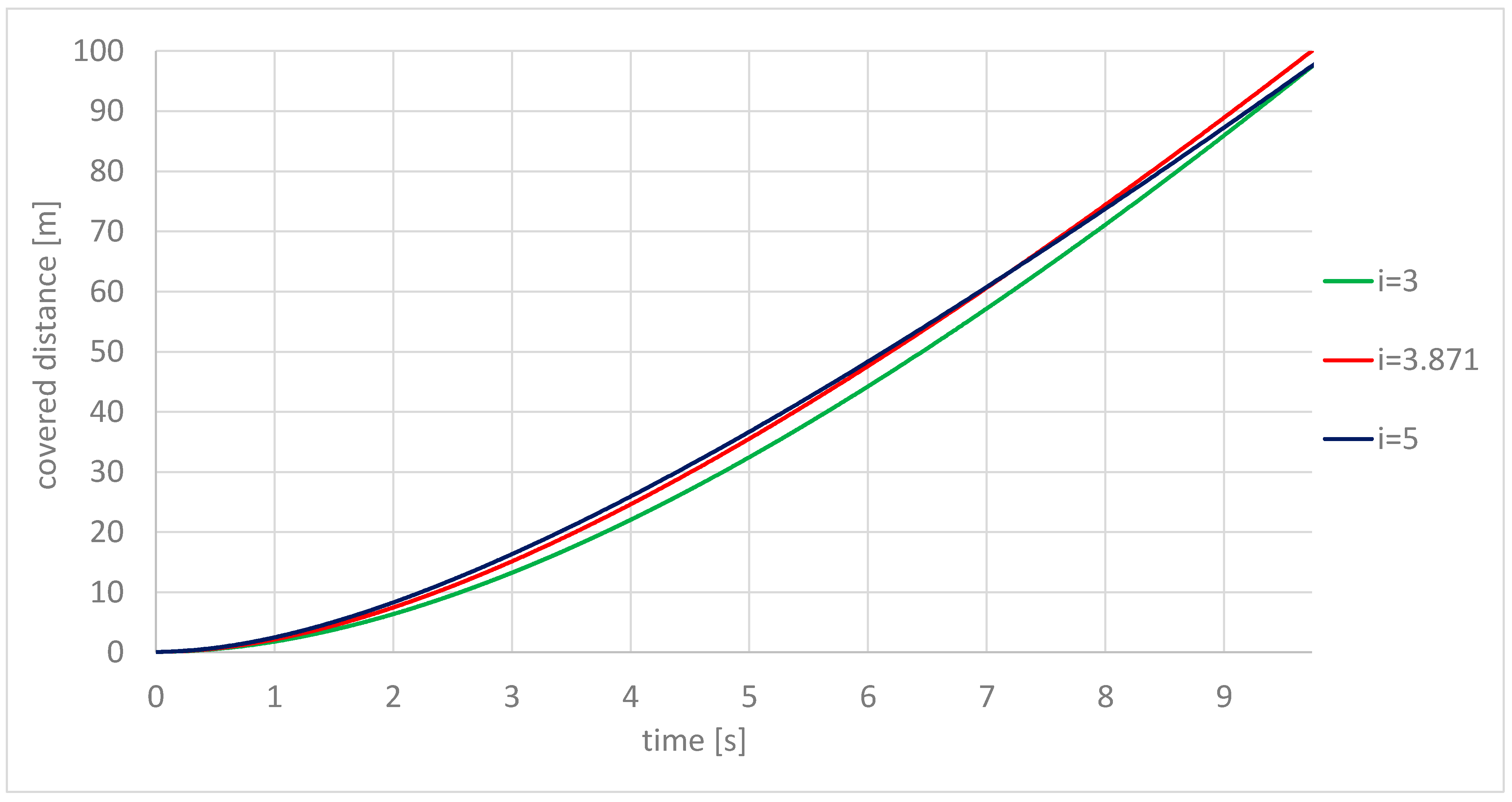
2. Brief Description of the Applied Vehicle Dynamics Model and Simulation Program

The filtering methodology introduced in this study is applied to the input parameters of a custom-developed vehicle dynamics simulation program tailored for prototype race cars [10]. Those input parameters whose minor variations do not significantly affect the simulation results relevant to the given competition task are filtered out. As a result, only the technical data that meaningfully influence vehicle performance are retained for optimization. We demonstrate the filtering process using our previously developed simulation program tailored for prototype race cars. This simulation program is based on our own vehicle dynamics model, the structure of which is shown in Figure 1. It is important to note that the proposed filtering approach is not limited to this particular model and can be extended to other vehicle dynamics simulation platforms.

The foundational model, shown in Figure 1, was developed for a single-seater, electrically powered prototype race car featuring a rigid frame and a drivetrain comprising a series-wound DC motor transmitting torque to the rear wheels via a chain drive. It must be remarked that the car has a rigid suspension, so the whole vehicle can be modeled as having a rigid frame structure. This model conceptualizes the vehicle as comprising four primary subsystems: the vehicle body, including the motor housing (stator), the motor rotor, the front and rear wheels, and associated rotating components. The relationship between the motor torque ($M_{motor}$) and the torque delivered to the rear wheels ($M_{wheel}$) is the following:

$$M_{wheel}=-\mathrm{ƞ}·i_{12}·M_{motor}$$

(1)

where

$$i_{12}={\displaystyle \frac{z_2}{z_1}}$$

(2)

The meaning of the notations in Equations (1) and (2) and in Figure 1 can be found in the Nomenclature.

The modeled race car was powered by a series-wound DC motor. The developed model of this motor [10] is shown in Figure 2.

Based on the models presented in Figure 1 and Figure 2, a complete vehicle dynamics simulation program was developed in MATLAB Simulink [10]. The modular structure of the simulation program is shown in Figure 3.

The complete simulation program, developed in MATLAB Simulink, is modular in structure (Figure 3), reflecting the logical organization of the dynamic model. It consists of five discrete modules: the vehicle body, front wheel assembly, rear wheel assembly, motor, and drivetrain. A comprehensive description of each module’s functionality and internal architecture can be found in [10]. In Section 3, a drag race is simulated, which is short in duration (~10 s), so thermal effects (e.g., changes in tire pressure due to tire heating) do not cause significant errors in the simulation. The maximum speed reached by the vehicle is not very high (~55 [km/h]), so errors resulting from aerodynamic changes are not significant.

The inputs of this program and its output functions are listed in the Nomenclature. The input data for the simulation include various vehicle and motor parameters. These may be sourced from the manufacturers’ catalogs and the scientific literature or determined through experimental measurement [38,39,40,41,42,43,44]. While certain data may be readily available, others can require custom measurement setups [45]. To address this, a bespoke experimental measurement system was developed and implemented, as described in [46].

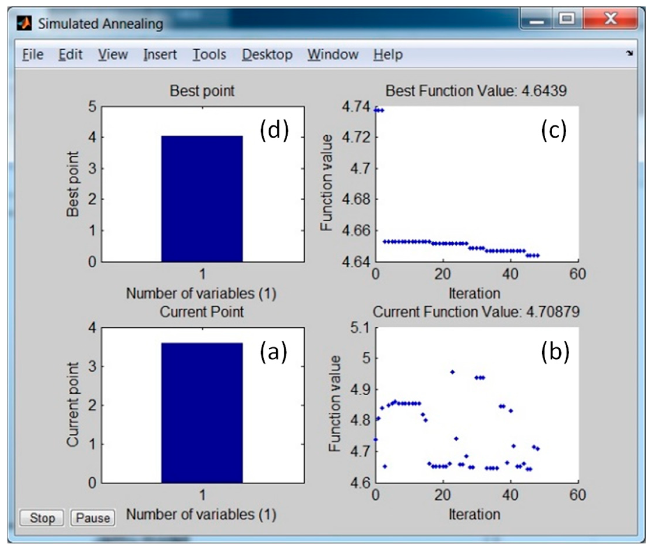
3. Brief Description of the Applied Optimization Method

The parameter optimization process implemented in our software comprises two distinct approaches: a graphical analysis method and an algorithmic technique based on Adaptive Simulated Annealing (ASA) [30]. While a comprehensive exposition of these methods is available in [11], this section provides a concise overview of the ASA-based approach, which plays a pivotal role in the framework.

The ASA method was realized using MATLAB’s Global Optimization Toolbox, specifically the “simulannealbnd” function, which is designed to perform bounded simulated annealing. To illustrate its application, we present an example optimization scenario: minimizing the time required for a race car to accelerate from a standstill to a velocity of 40 [km/h] by adjusting the gear ratio of the chain drive ($i_{12}$). The first step was to create a MATLAB function that calculates the time required to reach a speed of 40 [km/h], applying different gear ratios. The program code developed for this is shown in Figure A1. Using the above MATLAB code, the program code for optimization with the ASA method is shown in Figure A2 (Figure A1 and Figure A2 can be found in the Appendix A).

The codes in Figure A1 and Figure A2 determine the optimal gear ratio and the corresponding acceleration time to reach 40 [km/h]. During execution, the program outputs dynamic visual feedback, including (a) the current value of the optimization variable, (b) the calculated time for each tested ratio, (c) the evolution of the minimum time over iterations, and (d) the best solution found to that point—all visualized in Figure 4. Upon completion, the optimal gear ratio ($i_{12}=4.03$) and corresponding acceleration time ($t_{min}=4.64 \left[\mathrm{s}\right]$) are displayed in the command window.

To emphasize the practical implications of parameter optimization, another use case is presented. In this scenario, the objective is to minimize the time required to complete a 100 m drag race. Again, the chain drive gear ratio is selected as the optimization variable. Figure 5 illustrates the vehicle’s distance–time functions resulting from three gear ratio configurations: the optimal value (3.871) and two suboptimal alternatives (3.0 and 5.0). This simulation clearly demonstrates that the optimal ratio yields a time advantage of approximately 0.3 s, a margin that can be decisive in competitive racing.

As previously discussed, it is neither necessary nor efficient to optimize all vehicle parameters indiscriminately. Many variables exhibit minimal influence on performance outcomes in specific competition contexts. Therefore, identifying the subset of influential parameters is essential. To this end, we introduce a systematic filtering process, described in detail in the following section, which determines which variables merit inclusion in the optimization process.

4. Description of the Filtering Process

The objective of the proposed filtering methodology is to streamline the optimization process by identifying and excluding those input parameters whose uncertainties exert negligible influence on the simulation outputs. This enables a focused optimization strategy, significantly reducing computational demands and experimental effort. The filtering process comprises two main stages: (1) assessing the propagation of input uncertainties into simulation outputs and (2) determining thresholds for excluding non-influential parameters from the optimization.

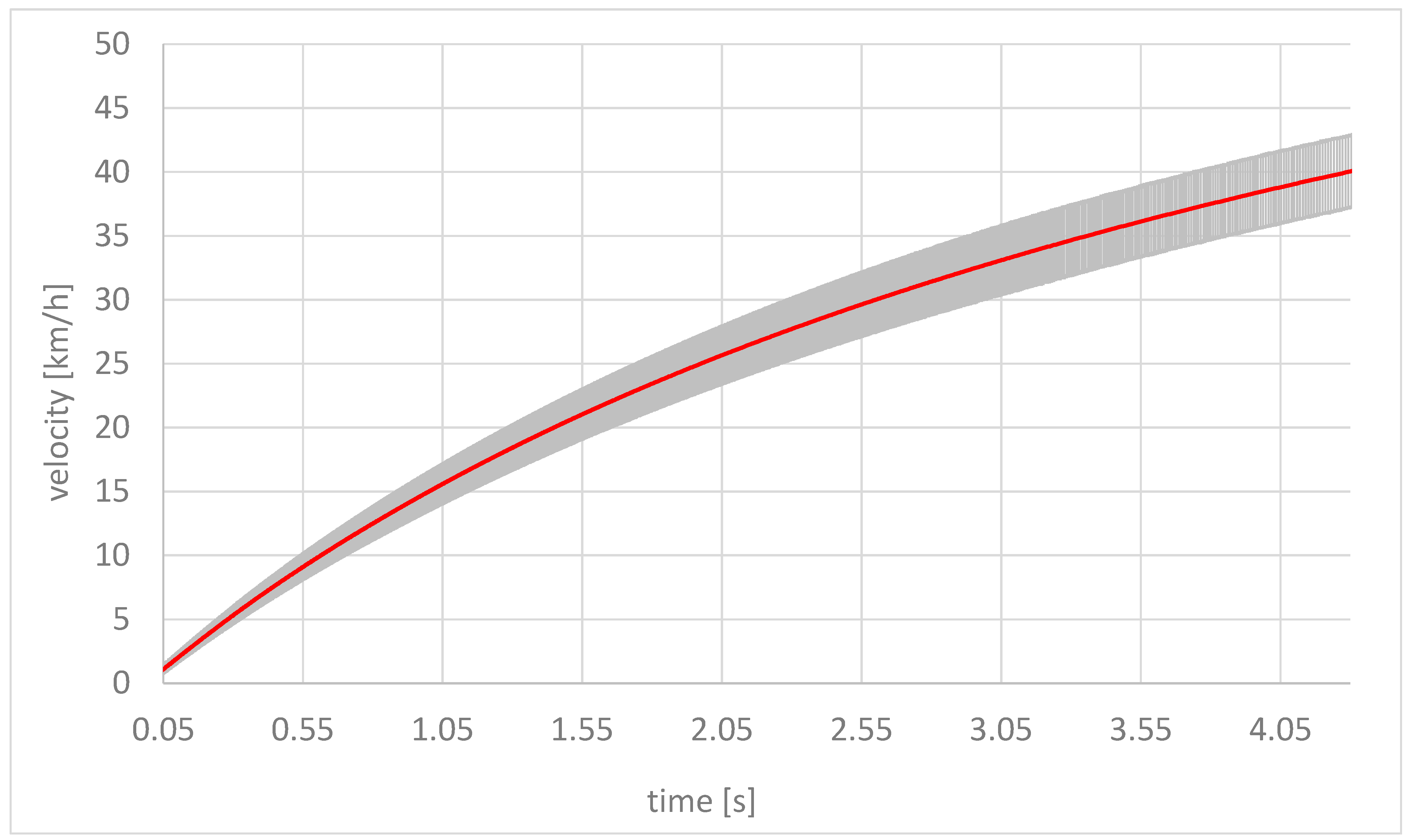
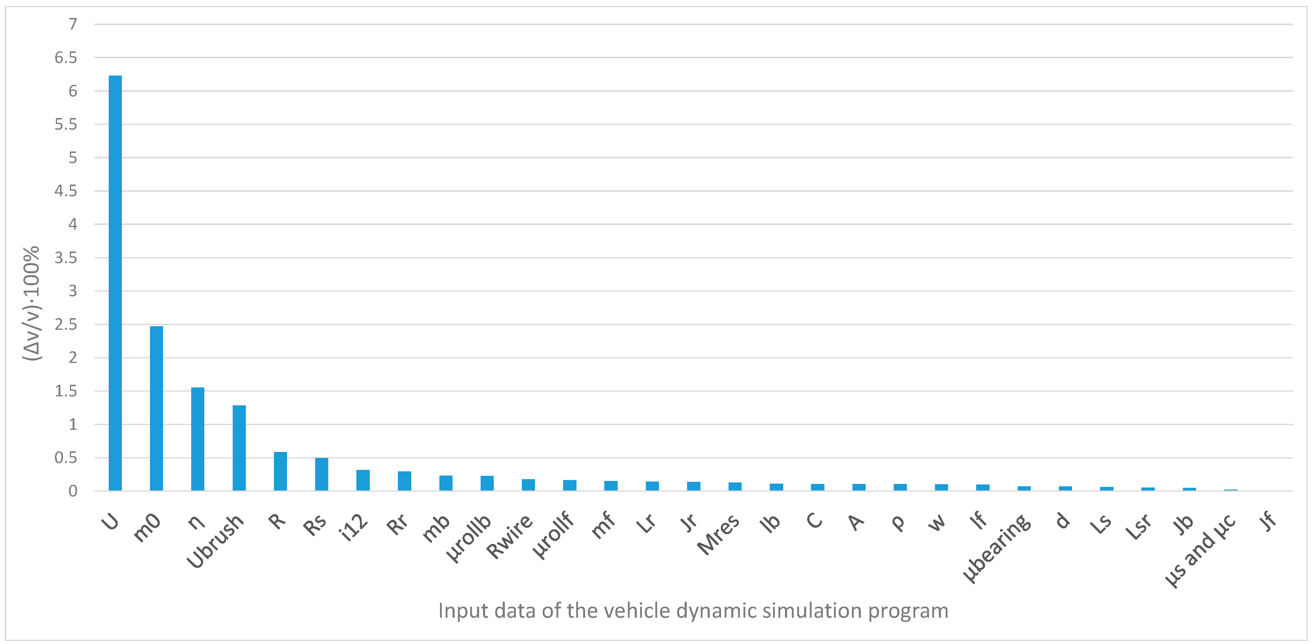
4.1. Determination of the Uncertainties of the Simulated Values

As a preliminary step, we evaluated the sensitivity of the simulation results to uncertainties in the input parameters. Specifically, we analyzed how the uncertainty of each input propagates to the uncertainty of the vehicle speed calculated by the simulation using the Gaussian Error Propagation Law [47] (3). To illustrate this approach, we selected a scenario in which the vehicle accelerates from rest to 40 [km/h]. The estimated uncertainties of relevant input parameters—based on prior experimental data and the literature values—are listed in

Table 1. Estimated uncertainties of the input data.

${\mathit{l}}_{\mathit{f}}\left[\mathbf{m}\right]$	${\mathit{l}}_{\mathit{b}}\left[\mathbf{m}\right]$	$\mathit{w}\left[\mathbf{m}\right]$	${\mathit{m}}_0\left[\mathbf{k}\mathbf{g}\right]$	${\mathit{m}}_{\mathit{f}}\left[\mathbf{k}\mathbf{g}\right]$	${\mathit{m}}_{\mathit{b}}\left[\mathbf{k}\mathbf{g}\right]$
$0.735\pm 0.007$	$0.615\pm 0.030$	$0.240\pm 0.012$	$247.7\pm 0.500$	$8.000\pm 0.010$	$16.90\pm 0.017$
${\mathit{J}}_{\mathit{f}}\left[\mathbf{k}\mathbf{g}·{\mathbf{m}}^2\right]$	${\mathit{J}}_{\mathit{b}}\left[\mathbf{k}\mathbf{g}·{\mathbf{m}}^2\right]$	${\mathit{J}}_{\mathit{r}}\left[\mathbf{k}\mathbf{g}·{\mathbf{m}}^2\right]$	${\mathit{i}}_{12}$	$\mathit{\eta }$	$\mathit{R}$
$0.182\pm 0.010$	$0.230\pm 0.011$	$0.020\pm 0.001$	$4.000\pm 0.004$	$0.970\pm 0.020$	$0.220\pm 0.011$
$\mathit{C}$	$\mathit{A}\left[{\mathbf{m}}^2\right]$	${\mathit{\mu }}_{{\mathit{r}\mathit{o}\mathit{l}\mathit{l}}_{\mathit{f}}}$	${\mathit{\mu }}_{{\mathit{r}\mathit{o}\mathit{l}\mathit{l}}_{\mathit{b}}}$	${\mathit{\mu }}_{\mathit{b}\mathit{e}\mathit{a}\mathit{r}\mathit{i}\mathit{n}\mathit{g}}$	$\mathit{d}\left[\mathbf{m}\right]$
$0.300\pm 0.060$	$1.000\pm 0.100$	$0.014\pm 0.001$	$0.018\pm 0.002$	$0.002\pm 0.0002$	$0.025\pm 0.00002$
$\mathit{U}\left[\mathbf{V}\right]$	${\mathit{U}}_{\mathit{b}\mathit{r}\mathit{u}\mathit{s}\mathit{h}}\left[\mathbf{V}\right]$	${\mathit{R}}_{\mathit{r}}\left[\mathsf{\Omega }\right]$	${\mathit{R}}_{\mathit{s}}\left[\mathsf{\Omega }\right]$	${\mathit{R}}_{\mathit{w}\mathit{i}\mathit{r}\mathit{e}}\left[\mathsf{\Omega }\right]$	${\mathit{M}}_{\mathit{r}\mathit{e}\mathit{s}}\left[\mathbf{N}\mathbf{m}\right]$
$48.00\pm 2.400$	$1.200\pm 0.120$	$0.01\pm 0.0001$	$0.016\pm 0.0002$	$0.006\pm 0.0001$	$0.600\pm 0.030$
${\mathit{\rho }}_{\mathit{a}\mathit{i}\mathit{r}}\left[\mathbf{k}\mathbf{g}/{\mathbf{m}}^3\right]$	${\mathit{L}}_{\mathit{s}\mathit{r}}\left[\mathbf{H}\right]$	${\mathit{L}}_{\mathit{s}}\left[\mathbf{H}\right]$	${\mathit{L}}_{\mathit{r}}\left[\mathbf{H}\right]$	${\mathit{\mu }}_{\mathit{s}} \mathbf{a}\mathbf{n}\mathbf{d} {\mathit{\mu }}_{\mathit{c}}$
$1.200\pm 0.024$	$0.00120\pm 0.00012$	$0.000340\pm 0.000034$	$0.00010\pm 0.00001$	$0.90\pm 0.09 \mathrm{a}\mathrm{n}\mathrm{d}$  $0.74\pm 0.074$

. Using these data, the propagated uncertainties in the simulated vehicle speed were computed and are presented in Figure 6.

$$∆v_{\mathrm{s}}=\sqrt{{\sum }_{i=1}^n{\left({\displaystyle \frac{\partial v_s}{\partial x_i}}\right)}^2·{∆x}_i^2}$$

(3)

In Equation (3), $∆x_i$ and $∆v_{\mathrm{s}}$ denote the uncertainties of the input data $\left(x_i\right)$ and the simulated vehicle speed $\left(v_{\mathrm{s}}\right),$ respectively. Partial derivative ${\displaystyle \frac{\partial v_s}{\partial x_i}}$ was approximated by the ratio ${\displaystyle \frac{∆v_{si}}{{∆x}_i}}$, where $∆v_{si}$ and ${∆x}_i$ are the uncertainties that belong to the 5% relative uncertainty of variable $x_i$ if the uncertainties of the other variables are zero.

The definitions of the symbols used in Table 1 are provided in the Nomenclature section. The uncertainty values were estimated based on previous experimental measurements and relevant literature sources. The simulated vehicle speeds and their associated uncertainties, corresponding to the input data and uncertainty estimates from Table 1, are depicted in Figure 6.

The results indicate that the relative uncertainty of the simulated speed ranges from 5% to 9% within the analyzed velocity interval (1–40 [km/h]), confirming the model’s robustness while highlighting the variable sensitivity of the output to different inputs.

4.2. The Filtering Process

As an initial step, we calculated the uncertainty in the simulated maximum vehicle speed (40 [km/h]) caused by applying a 5% relative uncertainty to each input parameter individually while assuming zero uncertainty for all other parameters. The resulting relative uncertainties in the output are visualized in Figure 7. (The tabulated data can be found in

Table A1. Relative percentage uncertainties of the simulated maximum vehicle speed (40 [km/h]) caused by 5% uncertainties in each input data separately.

	U	m0	η	Ubrush	R	Rs	i12	Rr	mb	µrollb
(Δv/v)·100%	6.2301	2.4704	1.551279	1.2817	0.5853	0.4972	0.3157	0.294016	0.2319	0.2295
	Rwire	µrollf	mf	Lr	Jr	Mres	lb	C	A	ρ
(Δv/v)·100%	0.1774	0.1629	0.149842	0.138	0.1369	0.1283	0.1114	0.103202	0.1032	0.1032
	w	lf	µbearing	d	Ls	Lsr	Jb	µs and µc	Jf
(Δv/v)·100%	0.0984	0.0962	0.068368	0.0684	0.0585	0.0512	0.0464	0.020672	0.0036

in Appendix A).

It can be concluded that optimization should be restricted to those parameters whose induced uncertainties, as shown in Figure 7, are significant. It should be remarked here that the Gaussian error propagation method is very effective in early filtering, as it assumes linearity between inputs and outputs, but as a result, it can oversimplify the effect of nonlinear interactions inherent in vehicle dynamics. In the case where the simulated value is highly sensitive to the uncertainty of an input parameter, the calculated error might be inaccurate. Therefore, if, after filtering is performed assuming the linearity above, we are uncertain whether a parameter should be excluded from the optimization or not, then it can be advisable to perform the error calculation also with a nonlinear approximation for the given parameter.

As a second step, we demonstrated that to ensure a simulated vehicle speed uncertainty of less than 10%, the relative uncertainty caused by each input parameter must be limited to 2%, assuming that all inputs contribute equally. Figure 8 illustrates the relative uncertainties of each input parameter that would individually result in a 2% uncertainty in the simulated maximum vehicle speed (40 [km/h]). (The tabulated data can be found in

Table A2. Relative percentage uncertainties for each input data that cause a relative uncertainty of 2% in the maximum vehicle speed (40 [km/h]).

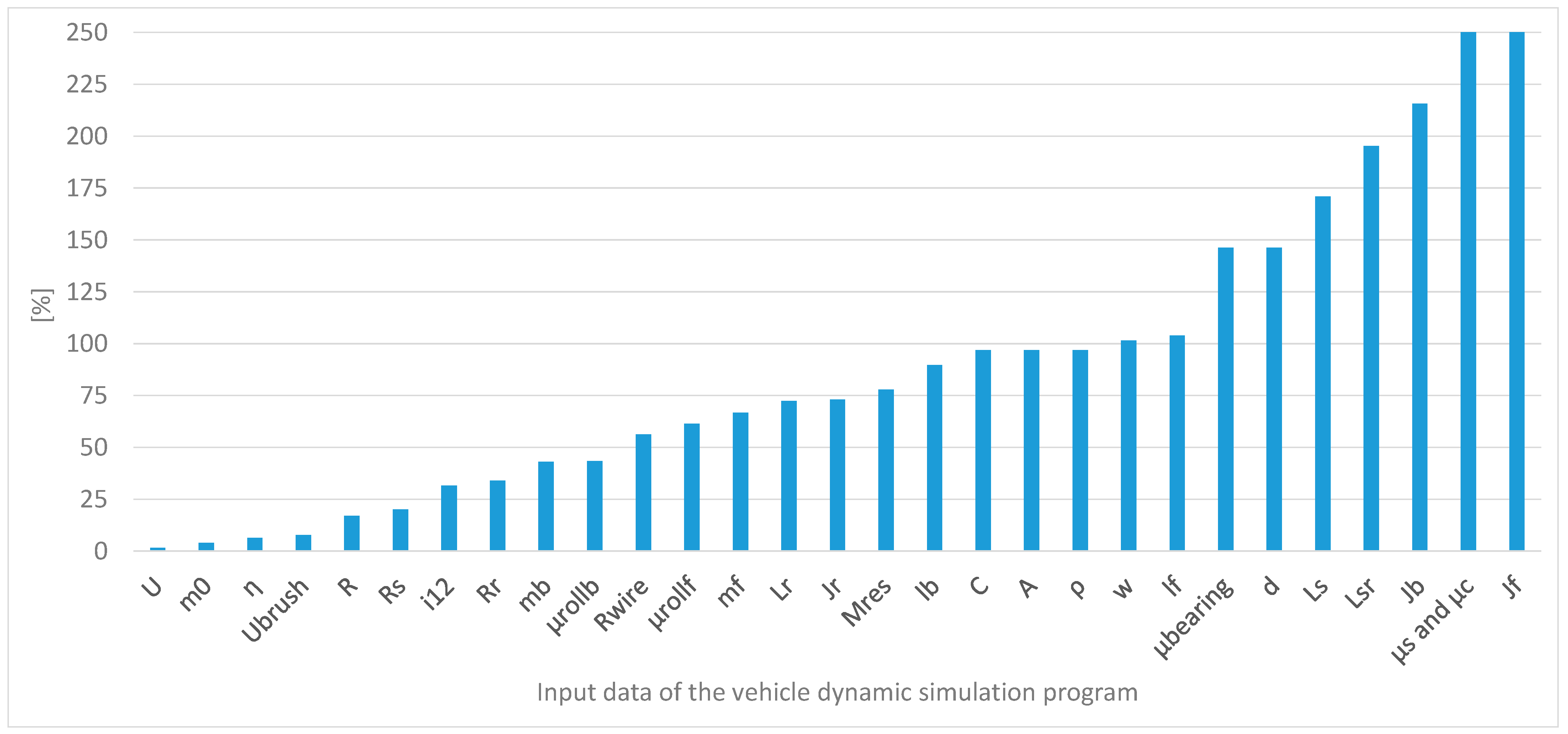
	U	m0	η	Ubrush	R	Rs	i12	Rr	mb	µrollb
%	1.6051	4.048	6.446293	7.8022	17.086	20.113	31.678	34.01172	43.125	43.573
	Rwire	µrollf	mf	Lr	Jr	Mres	lb	C	A	ρ
%	56.355	61.371	66.73718	72.459	73.061	77.949	89.771	96.89778	96.898	96.898
	w	lf	µbearing	d	Ls	Lsr	Jb	µs and µc	Jf
%	101.65	103.91	146.2675	146.27	171.05	195.35	215.67	483.7421	2796.4

in Appendix A).

As shown in Figure 8, the 2% uncertainty in the simulated vehicle speed is the result of applying 1.6% and 4% relative uncertainties to the battery terminal voltage ($U$) and the vehicle mass ($m_0$), respectively. The corresponding values for the electric resistance ($R_r$) and moment of inertia ($J_r$) of the rotor of the electric motor are 34% and 75%, respectively. Practically, this implies that the battery terminal voltage $\left(U\right)$ and vehicle mass $\left(m_0\right)$ must be determined with much greater precision than the electric resistance $\left(R_r\right)$ or moment of inertia $\left(J_r\right)$ of the rotor. Naturally, while all parameters should ideally be determined as accurately as possible, uncertainties of 20–30% in the electric resistance or the rotor’s moment of inertia would not introduce significant errors in the simulated vehicle speed.

In the example analyzed, it is advisable to maintain the input parameter uncertainties within or below the limits indicated in Figure 8. This requirement implies that the uncertainty in the battery terminal voltage $\left(U\right)$ should be ≤2%, potentially necessitating more detailed dynamic battery modeling [48,49] or measuring the battery terminal voltage in real-time during the drag race and then using these voltages as input data when running the simulation. It can be solved, e.g., by applying a NI 9239 voltage input module in real-time in in situ measurements. Regarding the vehicle mass $\left(m_0\right)$, an uncertainty of ≤4% is sufficient, which is easily achievable, as mass (${m_0,m}_f$ and $m_b$) can typically be measured with less than 1% uncertainty. It is advisable to know the chain drive efficiency ($\eta$) with an uncertainty of less than 7%, but according to the literature, it is typically known with an uncertainty of 2% or less [50]. In the case of the brush voltage ($U_{brush}$), an uncertainty of less than 8% is required, for which it is advisable to measure the value of the brush voltage as a function of the intensity of the current flowing through the motor as accurately as possible. The resistances of the motor windings ($R_r$ and $R_s$) should ideally have uncertainties of 20% or less, though, in practice, measurement accuracies better than 2% are readily achievable [38]. Similarly, uncertainties below 20% for the wheel radius ($R$) and gear ratio ($i_{12}$) are easily attainable.

The rolling resistance coefficients (${\mu }_{{roll}_f}$ and ${\mu }_{{roll}_b}$) should be known with uncertainties below 40%, achievable either through direct measurement or by using reliable literature estimates.

In the given example, it is sufficient to know the $L_r$, $J_r$, and $M_{res}$ characteristics of the motor with an uncertainty of less than 70% and the characteristics of $L_s$ and $L_{sr}$ with an uncertainty of less than 170% [38]. It should be emphasized that if the motor model itself is to be validated separately, considerably higher precision is required for these motor parameters, necessitating direct measurement if catalog data are unavailable [38,39,44,46].

For other inputs, estimated values may be safely used, and in some cases, parameters such as ${\mu }_{bearing}$ can even be omitted without introducing significant error into the simulation results. However, in other competition scenarios, a significantly higher level of accuracy may be necessary for certain parameters.

Overall, the parameters requiring precise knowledge vary according to the specific competition requirements. Consequently, for different competition tasks, the diagrams analogous to Figure 7 and Figure 8 would exhibit different uncertainty contributions for the same inputs.

Thus, prior to selecting optimization variables, it is essential to generate and interpret uncertainty diagrams similar to Figure 7 and Figure 8.

5. Summary

In this study, we have presented a modular software framework for simulating and optimizing the technical data of prototype race cars and introduced a novel filtering process to enhance the efficiency of parameter optimization. By quantifying the impact of input uncertainties on simulation results through error propagation, we identified which parameters significantly influence vehicle performance and which are the ones worth optimizing. This approach not only reduces computational time and effort but also provides practical guidance on measurement accuracy and the recommended measurement technique during experimental data collection. The use of MATLAB/Simulink combined with Adaptive Simulated Annealing after performing the presented filtering process proved to be an effective and practical solution for optimizing vehicle parameters in various competitive scenarios. Since no comparable filtering method was found in the existing literature, the proposed procedure represents a unique and valuable contribution to racing car design, supported by dynamic simulation and optimization.

During the filtering process, it was found that the parameters whose value most affects the vehicle’s travel time in the drag race presented in the example are the following: the battery terminal voltage, the vehicle mass, the chain drive efficiency and gear ratio, the wheel radius, the brush voltage, and the coil electrical resistance of the electric motor. Therefore, the parameters for which the optimization is performed must be selected from these.

In the near future, we plan to apply and test our filtering process under more complex dynamic scenarios (e.g., braking, cornering, and varying track conditions). Of course, to do this, we first need to further develop our simulation program or apply other available simulation programs. We also plan to investigate the possibility of integrating the filtering process into other available vehicle dynamics simulation programs. We also plan to test the applicability of other global optimizers, such as genetic algorithms or particle swarm optimization, and to perform a head-to-head comparison of the different methods under identical conditions.

References

- Juhász, G. A pneumobil versenyek és az oktatás—A felkészülés tanári szemmel. Debreceni Műszaki közlemények 2011, 1, 35–40, ISSN: 1587-9801. [Google Scholar]
- Gábora, A.; Sziki, G.Á.; Szántó, A.; Varga, T.A.; Magyari, A.; Balázs, D. Prototype battery electric car development for Shell-ECO-Marathon® competition. In Proceedings of the XXII International Conference of Young Engineers, Xi’an, China, 21–22 April 2017; pp. 167–170. [Google Scholar]
- Available online: https://www.shellecomarathon.com/ (accessed on 6 March 2025).
- Available online: https://pneumobil.hu/ (accessed on 6 March 2025).
- Rill, G.; Castro, A.A. Road Vehicle Dynamics: Fundamentals and Modeling with MATLAB®; CRC Press: Boca Raton, FL, USA, 2020. [Google Scholar]
- Shakouri, P.; Ordys, A.; Askari, M.; Laila, D.S. Longitudinal vehicle dynamics using Simulink/Matlab. In Proceedings of the UKACC International Conference on Control 2010, Coventry, UK, 7–10 September 2010; IET: Stevenage, UK, 2010; pp. 955–960. [Google Scholar]
- Vairavel, M.; Girimurugan, R.; Shilaja, C.; Loganathan, G.B.; Kumaresan, J. Modeling, validation and simulation of electric vehicles using MATLAB. In AIP Conference Proceedings; AIP Publishing: Melville, NY, USA, 2022; Volume 2452. [Google Scholar]
- Kıyaklı, A.O.; Solmaz, H. Modeling of an electric vehicle with MATLAB/Simulink. Int. J. Automot. Sci. Technol. 2019, 2, 9–15. [Google Scholar] [CrossRef]
- The MathWorks Inc. MATLAB Version: 9.13.0 (R2022b); The MathWorks Inc.: Natick, MA, USA, 2022; Available online: https://www.mathworks.com (accessed on 10 February 2025).
- Szántó, A.; Hajdu, S.; Sziki, G.Á. Dynamic simulation of a prototype race car driven by series wound DC motor in Matlab-Simulink. Acta Polytech. Hung 2020, 17, 103–122. [Google Scholar] [CrossRef]
- Szántó, A.; Hajdu, S.; Sziki, G.Á. Optimizing parameters for an electrical car employing vehicle dynamics simulation program. Appl. Sci. 2023, 13, 8897. [Google Scholar] [CrossRef]
- Li, P.; Löwe, K.; Arellano-Garcia, H.; Wozny, G. Integration of simulated annealing to a simulation tool for dynamic optimization of chemical processes. Chem. Eng. Process. 2000, 39, 357–363. [Google Scholar] [CrossRef]
- Vo, T.M.N. Centrifugal pump design: An optimization. Eurasia Proc. Sci. Technol. Eng. Math. 2022, 17, 136–151. [Google Scholar]
- Zadeh, L.A. Fuzzy logic. Computer 1988, 21, 83–93. [Google Scholar] [CrossRef]
- Adeli, H.; Sarma, K.C. Cost Optimization of Structures: Fuzzy Logic, Genetic Algorithms, and Parallel Computing; John Wiley & Sons: Hoboken, NJ, USA, 2006. [Google Scholar]
- Kim, J.; Kasabov, N. HyFIS: Adaptive neuro-fuzzy inference systems and their application to nonlinear dynamical systems. Neural Netw. 1999, 12, 1301–1319. [Google Scholar] [CrossRef]
- Elbaz, K.; Shen, S.L.; Zhou, A.; Yuan, D.J.; Xu, Y.S. Optimization of EPB shield performance with adaptive neuro-fuzzy inference system and genetic algorithm. Appl. Sci. 2019, 9, 780. [Google Scholar] [CrossRef]
- Karna, S.K.; Sahai, R. An overview on Taguchi method. Int. J. Eng. Math. Sci. 2012, 1, 1–7. [Google Scholar]
- Krishankant, J.T.; Bector, M.; Kumar, R. Application of Taguchi method for optimizing turning process by the effects of machining parameters. Int. J. Eng. Adv. Technol. 2012, 2, 263–274. [Google Scholar]
- Julong, D. Introduction to grey system theory. J. Grey system 1989, 1, 1–24. [Google Scholar]
- Li, Y.X.; Yang, J.G.; Gelvis, T.; Li, Y.Y. Optimization of measuring points for machine tool thermal error based on grey system theory. Int. J. Adv. Manuf. Technol. 2008, 35, 745–750. [Google Scholar] [CrossRef]
- Rao, R.V.; Savsani, V.J.; Vakharia, D.P. Teaching–learning-based optimization: A novel method for con-strained mechanical design optimization problems. Comput.-Aided Des. 2011, 43, 303–315. [Google Scholar] [CrossRef]
- Rao, R.V. Teaching-Learning-Based Optimization Algorithm; Springer International Publishing: Cham, Switzerland, 2016; pp. 9–39. [Google Scholar]
- Sivanandam, S.N.; Deepa, S.N.; Sivanandam, S.N.; Deepa, S.N. Genetic algorithm optimization problems. In Introduction to Genetic Algorithms; Springer International Publishing: Cham, Switzerland, 2008; pp. 165–209. [Google Scholar]
- Wang, D.; Tan, D.; Liu, L. Particle swarm optimization algorithm: An overview. Soft Comput. 2018, 22, 387–408. [Google Scholar] [CrossRef]
- Glover, F.; Kelly, J.P.; Laguna, M. Genetic algorithms and tabu search: Hybrids for optimization. Comput. Oper. Res. 1995, 22, 111–134. [Google Scholar] [CrossRef]
- Kirkpatrick, S.; Gelatt, C.D., Jr.; Vecchi, M.P. Optimization by simulated annealing. Science 1983, 220, 671–680. [Google Scholar] [CrossRef]
- Kirkpatrick, S. Optimization by simulated annealing: Quantitative studies. J. Stat. Phys. 1984, 34, 975–986. [Google Scholar] [CrossRef]
- Faber, R.; Jockenhövel, T.; Tsatsaronis, G. Dynamic optimization with simulated annealing. Comput. Chem. Eng. 2005, 29, 273–290. [Google Scholar] [CrossRef]
- Ingber, L. Adaptive simulated annealing (ASA): Lessons learned. Invit. Pap. A Spec. Issue Pol. J. Control Cybern. Simulated Annealing Appl. Comb. Optim. 1995, 25, 33–54. [Google Scholar]
- Eckert, J.J.; Santiciolli, F.M.; Silva, L.C.; Dedini, F.G. Vehicle drivetrain design multi-objective optimization. Mech. Mach. Theory 2021, 156, 104123. [Google Scholar] [CrossRef]
- Eckert, J.J.; Silva, L.C.; Costa, E.S.; Santiciolli, F.M.; Dedini, F.G.; Corrêa, F.C. Electric vehicle drivetrain optimisation. IET Electr. Syst. Transp. 2017, 7, 32–40. [Google Scholar] [CrossRef]
- Salvan, L.; Brüll, M.; Hollstein, A.; Medina, R.; Wilkins, S.; Avramis, N. Electric Drivetrain Optimization for 48V Urban Vehicles. In Proceedings of the 35th Electric Vehicle Symposium (EVS35), Oslo, Norway, 11–15 June 2022; pp. 1–13. [Google Scholar]
- Lu, M.; Domingues-Olavarría, G.; Márquez-Fernández, F.J.; Fyhr, P.; Alaküla, M. Electric drivetrain optimization for a commercial fleet with different degrees of electrical machine commonality. Energies 2021, 14, 2989. [Google Scholar] [CrossRef]
- Zhang, P.; Chen, Y.; Lin, M.; Ma, B. Optimum matching of electric vehicle powertrain. Energy Procedia 2016, 88, 894–900. [Google Scholar] [CrossRef]
- Li, C.; Cong, Z.; Zhang, B.; Jing, H. A Simulated Annealing algorithm based optimization for vehicle Powertrain Mounting System. In Proceedings of the 2015 5th International Conference on Information Science and Technology (ICIST), Changsha, China, 24–26 April 2015; IEEE: Piscataway, NJ, USA, 2015; pp. 10–13. [Google Scholar]
- Genc, M.O.; Kaya, N. Vibration Damping Optimization using Simulated Annealing Algorithm for Vehicle Powertrain System. Eng. Technol. Appl. Sci. Res. 2020, 10, 5164–5167. [Google Scholar] [CrossRef]
- Sziki, G.Á.; Sarvajcz, K.; Kiss, J.; Gál, T.; Szántó, A.; Gábora, A.; Husi, G. Experimental investigation of a series wound dc motor for modeling purpose in electric vehicles and mechatronics systems. Measurement 2017, 109, 111–118. [Google Scholar] [CrossRef]
- Szántó, A.; Kiss, J.; Mankovits, T.; Szíki, G.Á. Dynamic Test Measurements and Simulation on a Series Wound DC Motor. Appl. Sci. 2021, 11, 4542. [Google Scholar] [CrossRef]
- Pálinkás, S. Influence of Speed to Rolling Resistance Factor in Case of Autobus. In Vehicle and Automotive Engineering 4: Select Proceedings of the 4th VAE2022, Miskolc, Hungary; Springer International Publishing: Cham, Switzerland, 2022; pp. 157–164. [Google Scholar]
- Pálinkás, S.; Tóth, Á. Development of a measurement method to determine rolling resistance. In IOP Conference Series: Materials Science and Engineering; IOP Publishing: Bristol, UK, 2022; Volume 1237, p. 012013. [Google Scholar]
- Szíki, G.Á.; Szántó, A.; Mankovits, T. Dynamic modeling and simulation of a prototype race car in MATLAB/Simulink applying different types of electric motors. Int. Rev. Appl. Sci. Eng. 2021, 12, 57–63. [Google Scholar]
- Szántó, A.; Szántó, A.; Sziki, G.Á. Review of the modeling methods of series wound DC motors. Műszaki Tudományos Közlemények 2020, 13, 166–169. [Google Scholar]
- Szántó, A.; Ádámkó, É.; Juhász, G.; Sziki, G.Á. Simultaneous measurement of the moment of inertia and braking torque of electric motors applying additional inertia. Measurement 2022, 204, 112135. [Google Scholar] [CrossRef]
- Hadžiselimović, M.; Blaznik, M.; Štumberger, B.; Zagradišnik, I. Magnetically nonlinear dynamic model of a series wound DC motor. Przegląd Elektrotechniczny 2011, 87, 60–64. [Google Scholar]
- Sziki, G.Á.; Szántó, A.; Kiss, J.; Juhász, G.; Ádámkó, É. Measurement system for the experimental study and testing of electric motors at the faculty of engineering, University of Debrecen. Appl. Sci. 2022, 12, 10095. [Google Scholar] [CrossRef]
- Error Propagation Calculator. Available online: http://julianibus.de/ (accessed on 12 April 2025).
- Saldaña, G.; San Martín, J.I.; Zamora, I.; Asensio, F.J.; Oñederra, O. Analysis of the current electric battery models for electric vehicle simulation. Energies 2019, 12, 2750. [Google Scholar] [CrossRef]
- Tremblay, O.; Dessaint, L.A. Experimental validation of a battery dynamic model for EV applications. World Electr. Veh. J. 2009, 3, 289–298. [Google Scholar] [CrossRef]
- Pattantyús, Á.G. Gépész és Villamosmérnökök Kézikönyve 2; Műszaki Könyvkiadó: Budapest, Hungary, 1961. [Google Scholar]