Study on the Compressive Strength Predicting of Steel Fiber Reinforced Concrete Based on an Interpretable Deep Learning Method

Abstract

Steel fiber reinforced concrete (SFRC) exhibits excellent material enhancement and toughening properties. It is widely used in applications such as airport runways, highway pavements, and bridge deck overlays. In order to predict the compressive strength of SFRC efficiently and accurately, this study proposes a deep learning-based prediction model, trained and tested on a large set of experimental data. Additionally, the SHapley Additive exPlanations (SHAP) interpretability method is employed to analyze and interpret the prediction outcomes. SHAP facilitates the identification and visualization of both positive and negative correlations among input features, along with their magnitudes and overall importance from local and global perspectives. This analysis sheds light on the decision-making logic of the “black-box” model and addresses the transparency challenges typically associated with conventional machine learning (ML) approaches. Fourteen physical parameters, including steel fiber content, length, diameter, cement dosage, coarse aggregate content, and fly ash content, are selected as input features. The SHAP values of these parameters are visualized to assess their importance, impact, and influencing patterns on compressive strength prediction. The results show that the optimized deep learning model has higher prediction accuracy and generalization ability compared to other traditional ML models. The SHAP analysis results are consistent with the experimental results, and the predictive model well reflects the complex nonlinear relationship between various characteristic parameters, which can provide a basis and reference for the engineering design of SFRC materials.

1. Introduction

In recent years, the scale of highway construction in China has expanded rapidly. With the continuous increase in traffic volume and load ratings, various forms of pavement distress have emerged. To enhance the performance and durability of pavement structures, an increasing number of new materials and technologies have been adopted in highway construction. Among these, the incorporation of steel fibers into cement concrete or asphalt concrete has proven effective in improving pavement performance. Extensive engineering practice has demonstrated that adding steel fibers to cement concrete pavements can reduce slab thickness, minimize or eliminate the need for longitudinal joints, and reduce transverse contraction joints, while also offering excellent abrasion resistance and freeze–thaw resistance. Furthermore, steel fibers enhance the crack resistance and high-temperature rutting resistance of asphalt concrete, providing significant reinforcement and toughening benefits to pavement structures. Due to their high tensile strength, good toughness, and strong compatibility with concrete, steel fibers have become a widely demanded reinforcing material in practical engineering applications. Research has shown [1] that adding only 1–2% of steel fibers can significantly enhance the tensile strength, deformation property, energy dissipation capacity, and ductility of concrete. As a result, steel fiber reinforced concrete (SFRC) has been widely applied in various engineering fields, including pavement structures, bridge components, airport runways, tunnels, and hydraulic structures. Typical engineering applications include SFRC overlays, layered SFRC pavements, and SFRC-reinforced bridge piers and abutments, as well as shotcrete SFRC for stabilizing road slopes and tunnel linings.

The compressive strength of SFRC is a critical parameter for structure design and quality testing, which is generally obtained by testing standard cubic or cylindrical specimens, which consumes a large amount of raw materials and is very time-consuming to produce and maintain [2]. Moreover, in practical engineering applications, the results are often influenced by a variety of factors such as construction techniques and environmental conditions. Some researchers [3] have proposed some empirical formulas on an experimental basis with the help of linear or nonlinear statistical regression methods. Traditional empirical formulas are mostly based on linear or polynomial regression models, which typically involve a limited number of variables and oversimplify the underlying physical mechanisms. They often neglect the combined influence of multiple factors—such as fiber characteristics and material properties—on the compressive strength of steel fiber reinforced concrete, and are incapable of quantifying the complex interactions among these variables. Moreover, the development of such formulas usually depends on a limited set of experimental data. Although this often yields concise expressions that are convenient for practical application, the limited data scope significantly restricts their generalization capability. However, due to the complex composition of concrete materials and the interdependence among various influencing factors, the behavior of SFRC exhibits strong nonlinearity. At present, there is still a lack of systematic and accurate theoretical or experimental models that can comprehensively and reliably capture the relationships among the various factors affecting its compressive strength.

In recent years, with the emergence and development of artificial intelligence, machine learning (ML) provides new ideas and approaches for the rational prediction of SFRC [4]. ML is able to learn and mine potential laws directly from large amounts of data, and even approximate any continuous function [5] that connects input and output space with arbitrary accuracy. The current application of ML methods in civil engineering is also rapidly expanding. Torkan Shafighfard et al. [6] employed several ML models to predict the compressive strength of SFRC exposed to high-temperature environments, and comprehensively analyzed and discussed the application of each model and performance to obtain the optimal algorithm adapted to their specific dataset. Zhang et al. [7] established nine different ML models to predict the compressive strength of concrete and found that the nonlinear model showed better performance than the linear model. Yongjian Li et al. [8] employed two integrated methods (SVR AdaBoost and SVR Bagging) and Support Vector Regression (SVR) independent algorithms to predict the 28-day compressive strength of SFRC. Although these studies have achieved some good results in concrete strength prediction, ML is usually regarded as “black box” that is unable to provide sufficient justification for the results obtained by the model [9]. That is to say, the physical significance of such models is not clear, and they generally fail to clarify the relationship between input features and output results based on theoretical knowledge, which reduces the credibility and application of ML.

Based on the aforementioned limitations, the Shapley Additive exPlanations (SHAP) interpretable method and deep learning (DL) provide better solutions. Lundberg et al. [10] proposed the SHAP method for interpreting machine learning models based on game theory, which introduces the concept of additive interpretation to quantify the calculation of the contribution of each feature to the prediction result. The SHAP interpretability method not only provides accurate local explanations by clearly illustrating the direction and magnitude of each feature’s contribution in individual predictions, but also delivers global explanations by ranking the overall importance of input features. DL, as a kind of deep-level machine learning, can automatically perform high-dimensional abstract learning on the data through multilayer neural network architectures [11], which not only avoids the traditional ML model’s feature screening and dimensionality reduction on the original data before training, reduces the composition of the feature engineering, and saves time, but also has more advantages in the processing of the problem with a larger volume of data and a high degree of nonlinearity between the target variable and the input variable. The current application in the field of concrete mechanical property prediction is still relatively small. Therefore, based on a large amount of published relevant experimental data, this study establishes a prediction model using a deep learning algorithm to predict the compressive strength of SFRC, and uses the SHAP method to reveal the potential mechanism behind the model prediction results. By visualizing the SHAP values of feature parameters, the importance and influence of the input features on the compressive strength results were directly analyzed, and the influence of the feature parameters on the compressive strength of SFRC was provided as a basis and reference for the engineering design of SFRC materials.

2. Fundamental Principle and Main Formula

2.1. Deep Learning

Deep learning, which is based on artificial neural networks, broadly refers to a class of models characterized by multilayer network architectures. There are many kinds of existing deep learning structures. As the fundamental architecture of DL, the fully connected Deep Neural Network (DNN) is suitable for solving general data problems without special structure features and has strong generalization capability [12]. A typical framework of a deep neural network is illustrated in Figure 1.

The DNN propagates the input data forward through multiple layers, learning the hidden effective information between the input data. Neurons in each subsequent layer receive information from the preceding layer, which is processed through weighted summation and computation. The prediction error, calculated using a loss function, is then propagated backward through the network. At the same time, activation functions transmit the transformed outputs layer by layer toward the final output layer. In the whole process, the optimizer continuously updates the weights and biases between neurons, allowing prediction results to approximate the target values, and achieve the complex nonlinear mapping from input to output. Therefore, DNNs are capable of learning and simulating various complex problems in nature and engineering.

Assuming that the neural network consists of n hidden layers and the activation function is $\sigma$, the mapping relationship between the data of the j′th neuron in the i′th layer and the neurons in the previous layer can be expressed as follows:

$$z_j^i=\sigma \left[{\displaystyle \sum _{k-1}^{N_{i-1}}\left(W_{j,k}^i{z}_k^{i-1}+b_j^i\right)}\right]$$

(1)

where $W_{j,k}^i$ is the weight, $b_j^i$ is the bias value, and $N_{i-1}$ is the number of neurons in layer i − 1.

Assuming that the input feature of the neural network is X, the output feature is Y, and the parameter $\theta =\left[W,b\right]$ is to be determined by the neural network, the mapping relationship between the input and output layers of the neural network can be expressed as follows:

$$Y=N(X;\theta )$$

(2)

where $N(•;\theta )$ is the neural network symbol representation under the control of parameter $\theta$.

When the deep neural network is used to solve the problem, one of the keys to control the convergence and accuracy of the calculation is the selection of the loss function. The loss function can be generally expressed as follows:

$$\mathcal{l}oss={\displaystyle \frac{1}{N}}{{\displaystyle \sum _{i=1}^N\left(z-z^{\ast }\right)}}^2$$

(3)

where z* is the exact value of the output obtained by experiment or calculation, and z is the predicted value of the output.

By using the optimization algorithm to train the model for the dataset $D={\left\{X_i,Y_i\right\}}_{i-1}^{N_s}$ ($N_s$ is the size of the dataset) obtained by experiment or calculation, the value of the parameter $\theta$ to be identified in the neural network model can be obtained [13,14], thereby minimizing the loss function as closely as possible to its global minimum.

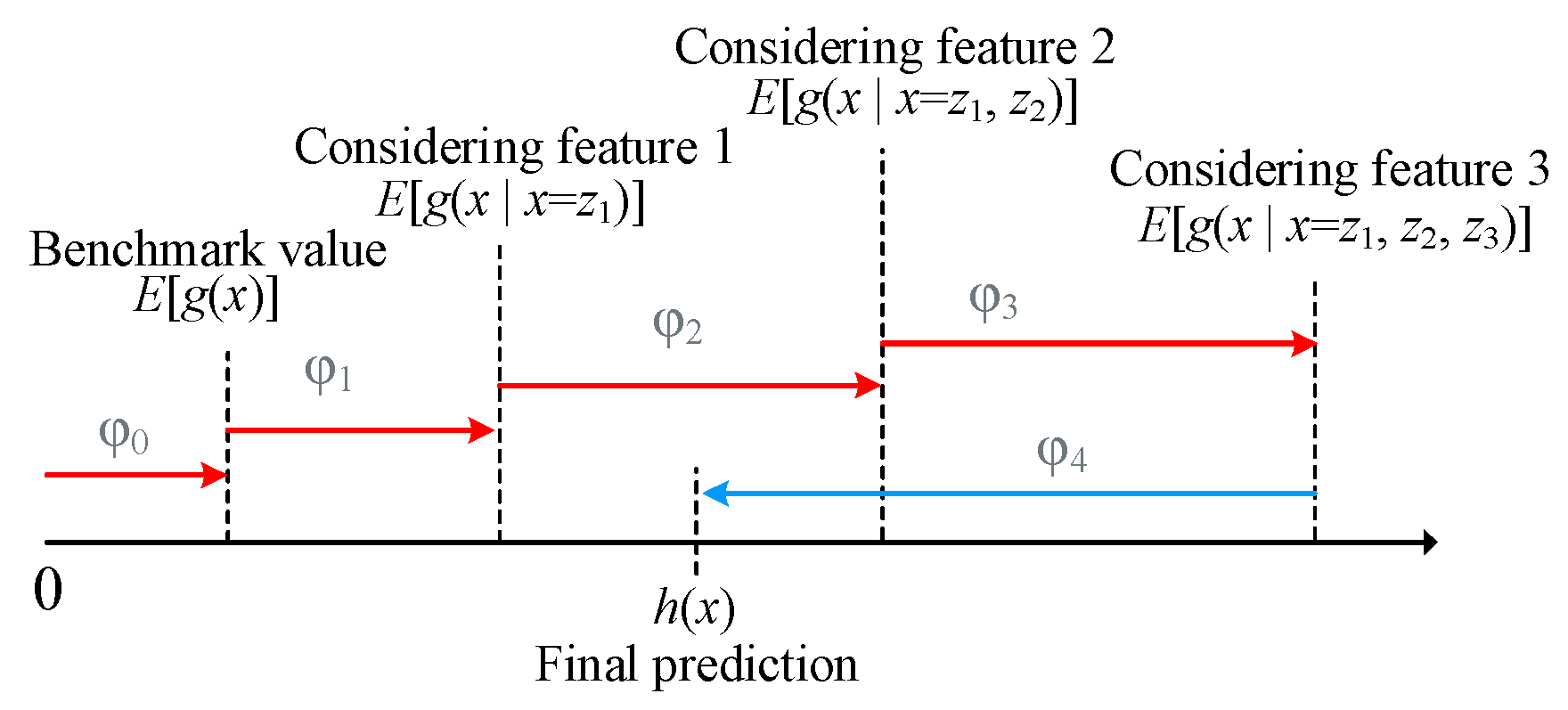
2.2. SHAP Interpretability Method

SHAP is a unified interpretable machine learning method proposed by Lundberg and Lee based on game theory. It interprets model predictions by calculating the contribution of each feature when added to the model, where the sum of all feature contributions equals the final output of the model. This approach effectively integrates both global and local interpretability [15]. In the SHAP method, the model output is based on the linear summation of the SHAP values of the input features, meaning that the effect of each input feature on the final prediction is quantified as a specific SHAP value, which can be expressed as follows:

$$h\left(x\right)=\mathrm{g}\left(x^{\prime }\right)={\phi }_0+{\displaystyle \sum _{i=1}^N{\phi }_i}{x}^{\prime }$$

(4)

where $h\left(x\right)$ represents the original prediction model; $\mathrm{g}\left(x^{\prime }\right)$ represents the corresponding interpretation model; x denotes the input feature; x′ represents the simplified input feature that are mapped to x; ${\phi }_0$ is the predicted mean of all samples, also known as the baseline; N represents the total number of features; and ${\phi }_i$ is the SHAP value of the i’th feature, which can be calculated by Equation (5).

$${\phi }_i(f,x)={\displaystyle \sum _{z^{\prime }\subseteq x^{\prime }}\frac{\left|z^{\prime }\right|!(N-\left|z^{\prime }\right|-1)!}{N!}\left[f_x(z^{\prime })-f_x(\frac{z^{\prime }}{i})\right]}$$

(5)

where N represents the feature complete set; z′ represents the feature subset; and $f_x(z^{\prime })=f_x(h_x(z^{\prime }))=E\left[g(x)\left|z_s\right.\right]$ represents the expected value on the subset z′.

Figure 2 briefly illustrates how SHAP analyzes the model to obtain the predicted value. It can be seen that SHAP interprets the final prediction of the model for the sample as the sum of the influence ${\phi }_i$ of each feature that introduces the conditional expectation. In the figure, red indicates that the feature contribution is positive, and blue indicates that the feature contribution is negative. Therefore, SHAP can quantify the influence of each feature in a given sample and its direction of correlation (positive or negative). It not only gives the importance of input features, but also shows how each feature affects the final prediction.

3. Model Construction and Prediction Results

3.1. Creation of the Experimental Results Database

As a crucial method for obtaining the mechanical properties of concrete under compressive stress, the uniaxial compression test plays an important role in understanding the mechanical behavior of concrete. At present, the uniaxial compression test of steel fiber reinforced concrete is carried out on a certain scale, but there are differences between the tests in various studies in the literature. In this study, a comprehensive database is compiled based on available uniaxial compression tests of SFRC, incorporating a sufficient amount of data extracted from the literature [8,16,17,18,19,20,21]. Following general data collection principles, the database is established with full consideration of various experimental influencing factors, including specimen composition, loading devices, and testing environments. A summary of the collected experimental data is presented as follows:

(1) Material aspect: All specimens use either ordinary Portland cement or Portland cement as the cement material. The aggregate is natural aggregate with good gradation and only one admixture of water reducing agent.

(2) Loading condition: The compressive strength values are either directly obtained from cube tests or converted from other specimen shapes to equivalent cube strength.

(3) Environment aspect: The specimens are standard maintenance to minimize the environmental impact as much as possible.

Each group of data contains the geometric size information of the specimen, the composition information of the concrete, the curing age, and the compressive strength. Based on these parameters, this study selects and combines 14 input features to predict the compressive strength of SFRC. These features include cement content, coarse aggregate content, fly ash content, slag content, silicon powder content, nano-silica content, limestone powder content, sand content, quartz powder content, water content, superplasticizer content, steel fiber content, steel fiber diameter, and steel fiber length. The statistical properties of the input features are shown in

Table 1. Statistical properties of the characteristic parameters.

Feature Parameter	Unit	Maximum	Minimum	Average	Standard Deviation
Cement content	kg/m3	1277.40	192.00	639.79	151.05
Fly ash content	kg/m3	989.57	0.00	34.60	356.14
Slag content	kg/m3	768.00	0.00	40.45	0.00
Silicon powder content	kg/m3	429.53	0.00	99.97	0.00
Nano-silica content	kg/m3	43.70	0.00	5.39	12.15
Limestone powder content	kg/m3	1058.20	0.00	50.66	0.00
Sand content	kg/m3	1503.40	407.80	951.13	265.05
Coarse aggregate content	kg/m3	1298.61	0.00	371.01	545.00
Quartz powder content	kg/m3	259.00	0.00	14.26	0.00
Water content	kg/m3	286.00	90.00	173.35	16.60
Dosage of high-range water reducer	kg/m3	92.04	0.00	24.32	5.45
Steel fiber content	%	8.00	0.00	1.28	0.75
Steel fiber diameter	mm	1.00	0.00	0.22	0.28
Steel fiber length	mm	60.00	0.00	14.57	17.50
Age	d	500.00	1.00	46.51	117.00

.

3.2. Deep Learning Model Construction

In this study, the TensorFlow deep learning platform is used. The hyperparameters that need to be set when establishing the model mainly include the number of hidden layers, the number of neurons, the activation function, the optimizer, the learning rate, the loss function, epoch, and batch_size.

For the selection of hidden layers and the number of neurons, too few may lead to underfitting, while too many can easily cause overfitting, resulting in poor generalization ability of the model. The activation function introduces nonlinear factors into the neural network. Common activation functions include sigmoid, tanh, relu, and Lrelu functions. In the process of deep learning back-propagation, the optimizer adjusts the parameters to minimize the loss function and approach the optimal solution. The commonly used optimizers include stochastic gradient descent (SGD), adaptive gradient (AdaGrad), adaptive moment estimation (Adam), root mean square propagation (RMSprop), etc. At present, there are many kinds of activation functions and optimizers, each of which has different characteristics. Selecting inappropriate activation functions and optimizers will have a significant negative impact on model performance. The learning rate determines the degree of change in the current weights during each update step. If it is too large, it may cause gradient oscillation and prevent the model from finding the global optimum; if it is too small, the convergence speed of the model becomes slow, resulting in longer training time. Regularization is used to prevent the model from overfitting. A commonly used method is Dropout regularization, which randomly deactivates a portion of neurons during each training iteration to reduce model complexity and enhance the diversity, sparsity, and generalization of the network. Usually, the model undergoes a certain number of epochs to converge, and an epoch indicates that all the training data have completed a forward computation and back-propagation process in the network.

Too small an epoch will lead to insufficient model training, and too large an epoch will lead to overfitting of the model. Usually, the value of the epoch is set to a larger value, and an early stopping strategy is adopted, that is, when the loss of the model on the training set is no longer decreased (the degree of reduction is lower than the predefined threshold), thereby avoiding the negative impact of excessive epochs on the model training process. Batch_size refers to the amount of data transmitted to the model for training in one iteration. If the batch_size is too small, the training speed will be slow and not easy to converge. A batch size that is too small can lead to slow training and unstable convergence, while a batch size that is too large may require more epochs to reach the same accuracy and may cause the model to converge to some bad local optimal points, although it can speed up the training process.

The hyperparameters of the model in this study are determined by the Bayesian optimization algorithm [22] except those that have been described and selected. The model is evaluated by five-fold cross-validation when adjusting the parameters. The dataset is randomly divided into a training set and test set according to the ratio of 7:3. The training set is substituted into the model for parameter determination and training. The test set only participates in the verification and evaluation of the accuracy and prediction performance of the final model. The final model hyperparameter values are shown in

Table 2. The hyperparameters of the model.

Parameter	Optimization Scope	Final Value
Number of hidden layers	1~10	3
Number of neurons	8~200	[32,136,168]
Activation function	relu, tanh, Lrelu	relu
Optimizer	SGD, Adam, RMSProp, AdaGrad	Adam
Rate of learning	[1,0.01,0.001,0.0001]	0.001
Regularization	-	Dropout
Epoch	-	3500
Batch_size	1~50	32

.

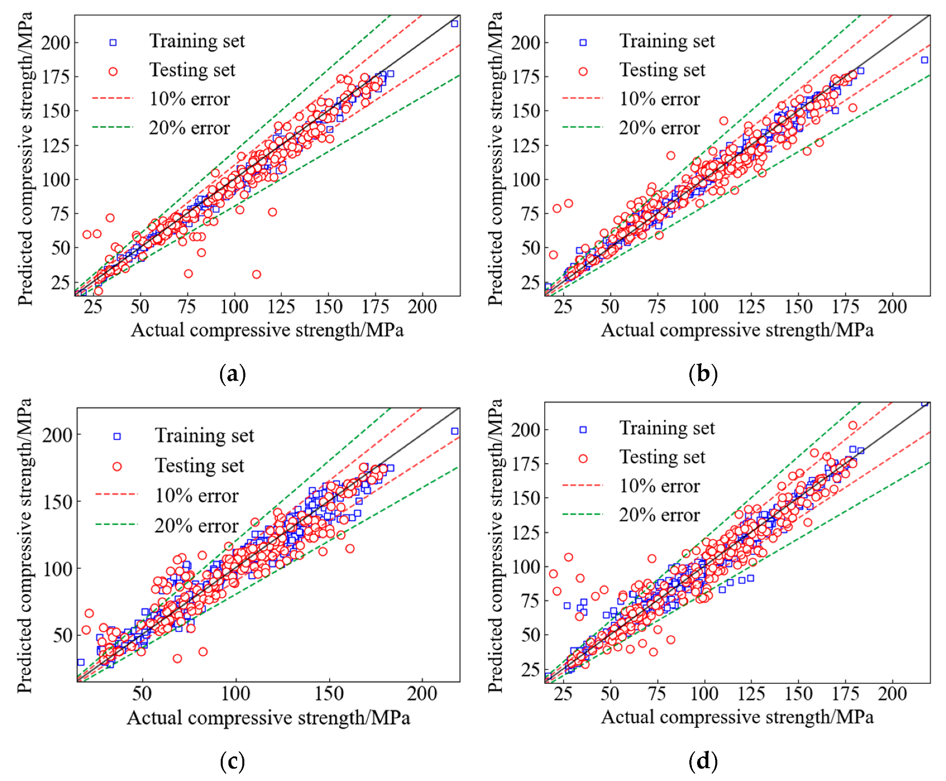
3.3. Comparison and Evaluation of Algorithm Model

In order to investigate the reliability and accuracy of the prediction results of the DNN model established in this study, under the same training and testing conditions, this paper uses three other commonly used algorithm models to compare them, which are extreme gradient boosting (XGBoost), random forest (RF), and back-propagation (BP) neural networks with only one hidden layer. After several iterations of training, the prediction of these four models on the training set and the testing set is obtained, as shown in Figure 3. It can be seen from Figure 3 that the DNN model has the best prediction effect. Except for individual sample points, most of the sample points can be closely distributed on both sides of the y = x line, followed by XGBoost and RF algorithm models, while the BP neural network model has a slightly weaker prediction ability.

There are many criteria for evaluating the performance of deep learning models. In this study, the widely used root mean square error (RMSE), mean absolute error (MAE), mean absolute percentage error (MAPE), and coefficient of determination (R²) are selected to evaluate the performance of the model. The calculation results are shown in

Table 3. Model performance evaluation.

Model	Training Set				Test Set
	R2	MAPE	RMSE	MAE	R2	MAPE	RMSE	MAE
DNN	0.9943	2.58%	2.95	2.22	0.9398	8.16%	9.41	6.62
RF	0.9892	3.04%	3.93	2.63	0.9179	10.33%	11.17	7.58
XGBoost	0.9417	8.27%	9.11	6.81	0.8804	11.31%	13.39	9.77
BP	0.9593	6.40%	7.79	4.35	0.8900	9.63%	12.32	8.86

. The closer the R² of the model is to 1, the smaller the RMSE, MAPE, and MAE, the better the fitting effect of the model and the smaller the prediction error. According to the evaluation index of the model, the DNN model proposed in this paper demonstrates the best predictive performance.

3.4. Comparison and Evaluation of Empirical Formulas

To verify the accuracy and reliability of the model presented in this paper, three classic empirical formulas for concrete failure criteria commonly used in practice were compared and analyzed, namely, the following:

(1) The formula for calculating the compressive strength of SFRC in China’s Code for Design of Concrete Structures (GB 50010-10) [23] is as follows:

$$f_{cu}=k{f}_{c0}+a{V}_f$$

(6)

(2) The American Concrete Institute’s Guide to Design with Fiber-Reinforced Concrete (ACI 544.4R-18) [24] provides specifications and design considerations for SFRC:

$$f_{cu}=0.97f_{c0}{V}_m+494V_{f}l/d$$

(7)

(3) CEB-FIP [25] recommended the following calculation formula:

$$f_{cu}=k{f}_{c0}+a{V}_f+b{V}_f^2$$

(8)

where f_cu is the compressive strength of steel fiber reinforced concrete; f_c0 is the compressive strength of ordinary concrete, $f_{c0}={\displaystyle \frac{A}{B^{w/c}}}\left(1+{\displaystyle \frac{t}{28}}\right)$; V_f is the steel fiber volume fraction; V_m = 1 − V_f; and k, a, b are material parameters, required experimental data fitting.

These three classical and widely used SFRC strength prediction models are used to carry out numerical calculations on the testing set data one by one. The numerical calculation results of each strength prediction model and the prediction results of the deep learning model in this study are consistent with the real test data, as shown in Figure 4. According to the visual analysis in Figure 4, the model proposed by the Chinese and American specifications is consistent, but with large errors, while the C-F model demonstrates the lowest accuracy. However, the dispersion of compressive strength predicted by the DNN model is smaller than that of these three classical strength prediction models, indicating better accuracy and reliability. It can be concluded that the DNN model established in this study can predict the compressive strength of SFRC more efficiently than the classical strength prediction model, and has better applicability. In addition,

Table 4. Model performance evaluation of the DNN model with these three classical strength formulas.

Model	Evaluation Indicators
	MAPE/%	RMSE/MPa	MAE/MPa
DNN	8.16	9.41	6.62
GB 50010	69.32	81.10	57.00
ACI 544.4R	58.10	58.10	56.00
CEB-FIP	453.12	820.90	391.28

shows the evaluation indicators on the testing set of the DNN model with these three classical strength formulas. According to the performance of each evaluation index, the DNN model exhibits superior accuracy and stronger predictive capability compared to classical strength formulas.

4. Interpretable Analysis of Prediction Model Based on SHAP

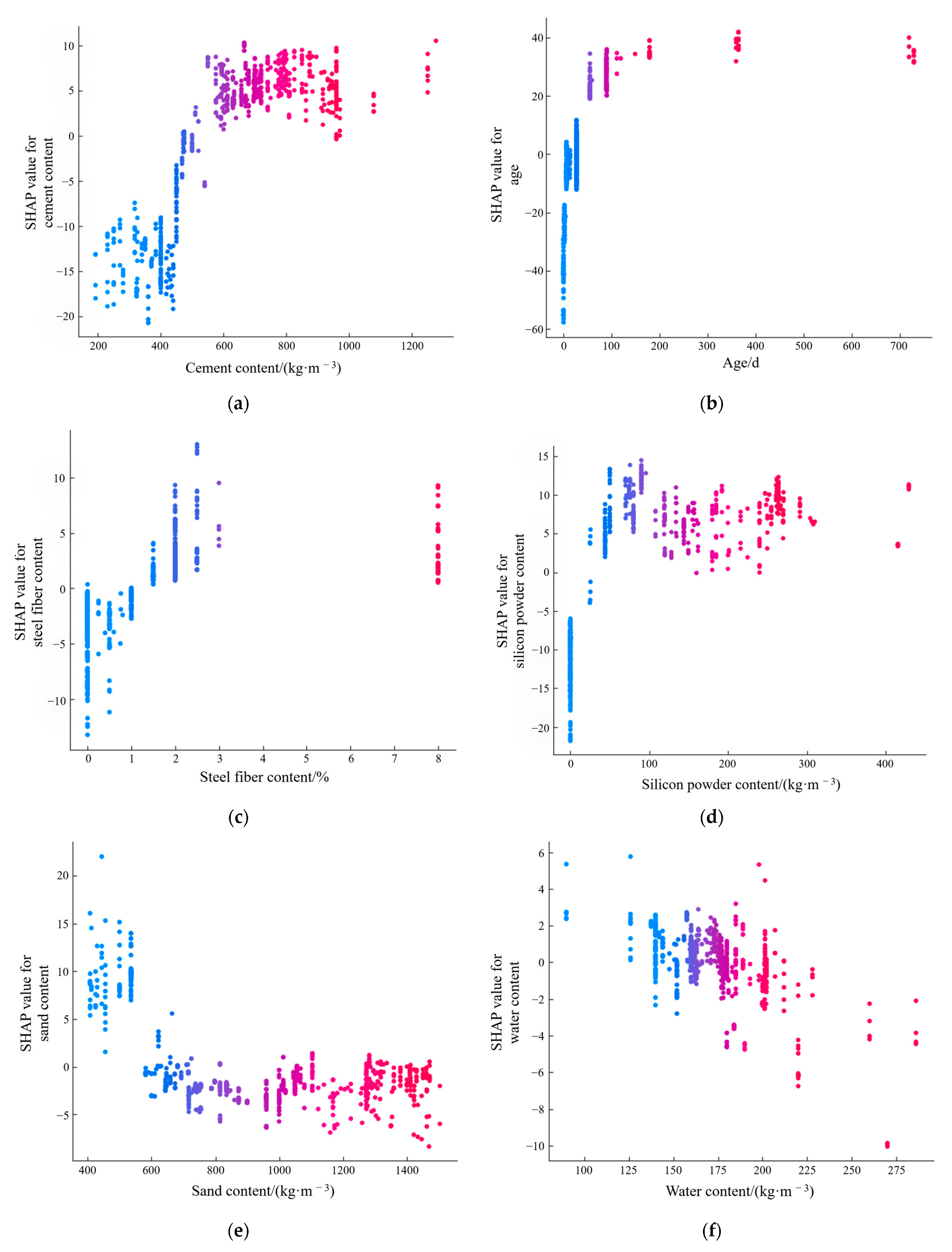
4.1. Partial Interpretation Based on SHAP

The purpose of local interpretation is to analyze and interpret the prediction results of a single sample. In this study, three samples were selected for local interpretation, taken from A3 (28-day age, 0.5% volume fraction of steel fiber), A5a (28-day age, 1.5% volume fraction of steel fiber), and A5b (90-day age, 1.5% volume fraction of steel fiber) in Reference [17]. The specific data are shown in

Table 5. Data of test samples.

Feature Parameter/Unit	Sample1 (A3)	Sample2 (A5a)	Sample3 (A5b)
Cement content/kg·m−3	400	400	400
Fly ash content/kg·m−3	0	0	0
Slag content/kg·m−3	0	0	0
Silicon powder content/kg·m−3	0	0	0
Nano-silica content/kg·m−3	0	0	0
Limestone powder content/kg·m−3	0	0	0
Sand content/kg·m−3	751	740	740
Coarse aggregate content/kg·m−3	1127	1111	1111
Quartz powder content/kg·m−3	0	0	0
Water content/kg·m−3	140	140	140
Dosage of high-range water reducer/kg·m−3	24.42	24.15	24.15
Steel fiber content/%	0.5	1.5	1.5
Steel fiber diameter/mm	0.55	0.55	0.55
Steel fiber length/mm	35	35	35
Age/d	28	28	90
Compressive strength/MPa	78.2	81	89.3

. From Formula (2), the final prediction of compressive strength is the result of the SHAP values of each input feature offsetting each other at the reference value. Here, the process of visual offsetting is visualized by the force plot, where the red and blue strips represent the positive and negative effects on the compressive strength, respectively. The length of the color strip represents the SHAP value of the feature, that is, the corresponding influence degree. Figure 5 is the force diagram of the three sample specimens.

For sample 1, the predicted compressive strength of the DNN model is 77.33 MPa, which is in good agreement with the test result of 78.2 MPa. As shown in Figure 5a, the final compressive strength is the positive and negative superposition of SHAP values of each input feature based on the reference value of 101.7 MPa. Features located in the blue region indicate a negative contribution relative to the baseline value, while those in the red region indicate a positive contribution. The longer the feature’s band, the greater its contribution and the more significant its influence. It can be seen from the figure that the cement content, coarse aggregate content, and the steel fiber length are the main characteristics of negative effect, while the dosage of high-range water reducer and water content are the main characteristics of positive effect. Cement content exhibits the strongest negative impact, whereas the dosage of high-range water reducer shows the most pronounced positive effect. Since the volume of steel fiber content in this sample is small (0.5%), the influencing factors of the final compressive strength are basically the same as those of ordinary concrete, including the cement content that determines the strength of the matrix, the coarse aggregate content, the superplasticizer content, and the water content, which significantly affect the mechanical properties of the composite material, which is consistent with the basic theoretical knowledge of concrete formed by long-term practice.

For sample 2, the predicted compressive strength of the DNN model is 80.65 MPa, which is very close to the experimental result of 81.0 MPa. As shown in the figure, cement content and coarse aggregate content, located in the blue region, are the main features exerting negative influence. Among them, cement content has the longest band, indicating the strongest negative impact. In contrast, the dosage of high-range water reducer and water content, located in the red region, are the primary features contributing positively, with the dosage of high-range water reducer having the longest band and thus the most significant positive effect. Compared with sample 1, the steel fiber content (1.5%) in sample 2 increases more. Therefore, it can be seen from Figure 5b that the content of steel fiber has become a major feature affecting the compressive strength of concrete and plays a positive role, which is consistent with the results of many experimental studies [17,19]. From the perspective of mechanism analysis, the appropriate amount of steel fiber incorporation can hinder the expansion of micro-cracks in concrete and block the occurrence and development of macro-cracks. This enhances the overall internal bonding performance of the concrete and improves its lateral confinement under compression. The confinement effect has improved the compressive strength of concrete to a certain extent.

For sample 3, the predicted compressive strength of the DNN model is 86.38 MPa, which is not much different from the test result of 89.3 MPa. As shown in the figure, cement content and coarse aggregate content, located in the blue region, are the main features exerting negative influence. In contrast, curing age, located in the red region, is the dominant feature with a positive effect, as indicated by its longest band length, representing the most significant positive contribution. The main difference between sample 3 and sample 2 is that the curing age is different (90 days and 28 days). Comparing Figure 5b,c, it can be seen that the curing age becomes a main feature affecting the compressive strength of concrete and plays a positive role, which means that under the same other conditions, prolonging the curing age allows the SFRC to achieve higher compressive strength. From the mechanism analysis, since the reaction of fine aggregate is relatively slow, the hydration product Ca(OH)₂ of cement is needed as the activator, and the fine aggregate will show an obvious enhancement effect in the later stage of cement hydration (generally after 28 days).

The SHAP analysis results of the above three samples show that appropriate steel fiber content and longer age contribute to the development of higher compressive strength of concrete.

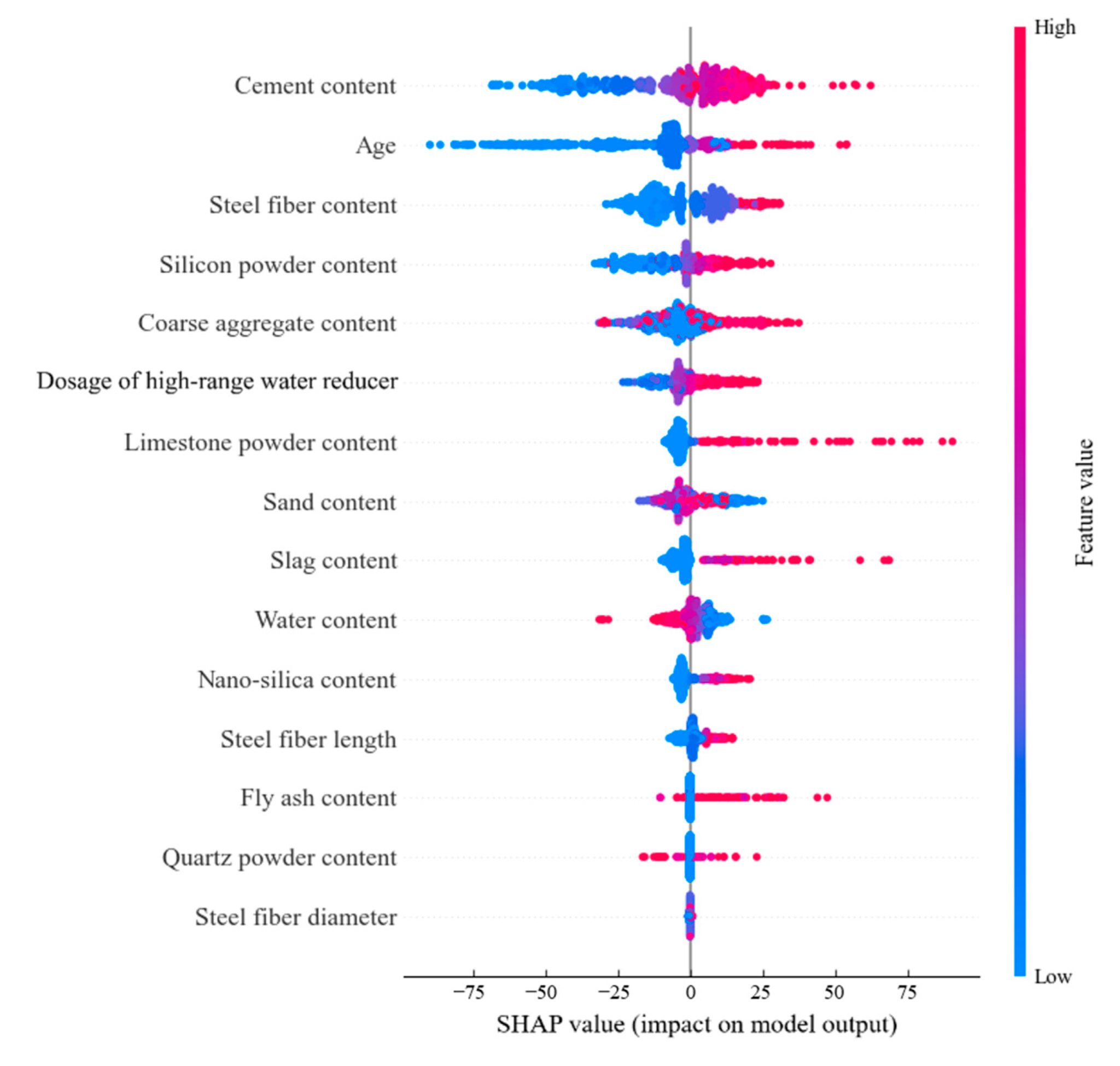
4.2. Global Interpretation Based on SHAP

The global interpretation aims to provide a comprehensive representation of SHAP values for the input features of all samples. Figure 6 shows the distribution of SHAP values for individual features throughout the dataset, where the vertical axis represents the input features ranked by importance, and the horizontal axis represents the SHAP values of specific features. Positive and negative values represent the positive and negative effects on the output results, respectively. The larger the absolute value, the higher the influence. The color represents the magnitude of the feature parameter values, with blue indicating lower values and red indicating higher values. Therefore, Figure 6 not only reflects the importance of characteristic parameters, but also reveals how changes in characteristic values affect the compressive strength of SFRC. It can be seen from Figure 6 that the cement content is the most important characteristic parameter affecting the compressive strength, which is consistent with the conclusion obtained in the local interpretation. The positive effect of cement content on the compressive strength of SFRC increases with the increase in characteristic parameter values. Similarly, as values of age, steel fiber content, silica powder content, coarse aggregate content, and dosage of high-range water reducer water reducer increase, their corresponding positive SHAP values also increase, indicating that these parameters have a positive effect on the compressive strength of SFRC. In contrast, water content and steel fiber length exhibit increasingly negative SHAP values as their values increase, suggesting a more significant negative impact on compressive strength. The influence of slag content on compressive strength shows a trend of first increasing and then decreasing. When the substitution rate of slag admixture for cement is too high, it will inevitably lead to a decrease in the amount of cement, a decrease in the content of Ca(OH)₂ that plays an activating role, and a deterioration of the hydration conditions of slag. Therefore, a higher slag substitution rate does not necessarily yield better results.

Figure 7 presents the dependence diagram of eight important characteristic parameters. Through the dependence diagram, the influence of parameter value change on compressive strength can be understood more deeply. The DNN model captures the overall relationship between these eight parameters on the compressive strength: (1) increases in age, steel fiber content, silica powder content, coarse aggregate content, and dosage of high-range water reducer lead to higher predicted compressive strength; (2) increases in water content, sand content, and steel fiber length result in a reduction in the predicted compressive strength.

From Figure 7a, it can also be clearly seen that the cement content is positively correlated with the compressive strength of SFRC. After the amount of cement reaches 600 kg/m³, the SHAP value becomes positive, and the positive impact on the compressive strength increases. It can be seen from Figure 7b that the SHAP value of the age increases with increasing curing time, with a rapid rise before 28 days and a slower increase thereafter, which is consistent with the hydration reaction process of the concrete. As shown in Figure 7c, when the steel fiber content reaches 2.5%, the SHAP value is positive and at its maximum, which has the greatest positive impact on the compressive strength. Steel fibers primarily enhance the toughness and failure behavior of concrete by inhibiting crack propagation. An increase in steel fiber content can improve the compressive strength of SFRC to a certain extent. However, since the matrix strength remains the dominant factor, this improvement is limited. As shown in Figure 7h, steel fiber length exhibits a nonlinear relationship with compressive strength. When the length is between 20 and 30 mm, the SHAP value is positive, indicating a slight enhancement in compressive strength. For lengths between 30 and 40 mm, the SHAP value tends to be neutral, and the improvement in strength becomes more apparent. However, when the length exceeds 50 mm, the excessive increase in fiber length negatively affects the workability and compaction of the concrete, ultimately weakening its compressive strength.

As shown in Figure 7d, when the silicon powder content is higher than 30 kg/m³, the SHAP value of silicon powder is larger than 0, which has a positive contribution to the predicted compressive strength. However, when the silicon powder content is higher than 40 kg/m³, the SHAP value decreases slightly. Excessive silicon powder, due to its large surface area, may reduce compressive strength; therefore, the silicon powder content should not be too high. Figure 7e shows that when the sand content is higher than 600 kg/m³, the SHAP value is less than 0, which indicates that the further addition of sand content will lead to a decrease in the compressive strength of SFRC.

Figure 7f,g show that the water content is negatively correlated with the compressive strength of SFRC. When the water content is low, higher dosage of high-range water reducer is required to achieve high strength. However, when the dosage of high-range water reducer exceeds 8 kg/m³, it begins to have a positive effect on compressive strength, reaching its maximum effect at around 18 kg/m³. It should be noted that the results in this study are based on the experimental data from the established literature database, and the situation outside the database (see Table 1 for parameter range) may need further discussion.

5. Conclusions

In this study, a deep learning model is proposed to predict the compressive strength of SFRC. Based on a massive number of experimental data, the model is trained and tested, and the prediction results are explained and analyzed by the SHAP interpretability method to overcome the “black-box” problem of conventional machine learning. The main conclusions are as follows:

• Model performance verification: The DNN model established in this study is compared and analyzed against three commonly used algorithmic models and three widely used empirical formulas. On the testing set, the model achieves an R² of 0.94 and a MAPE of 8.16%, indicating that the predicted compressive strength of SFRC is highly consistent with the experimental results. This demonstrates that the DL model proposed in this paper possesses high prediction accuracy and generalization ability, and effectively captures the complex nonlinear relationships among the characteristic parameters.
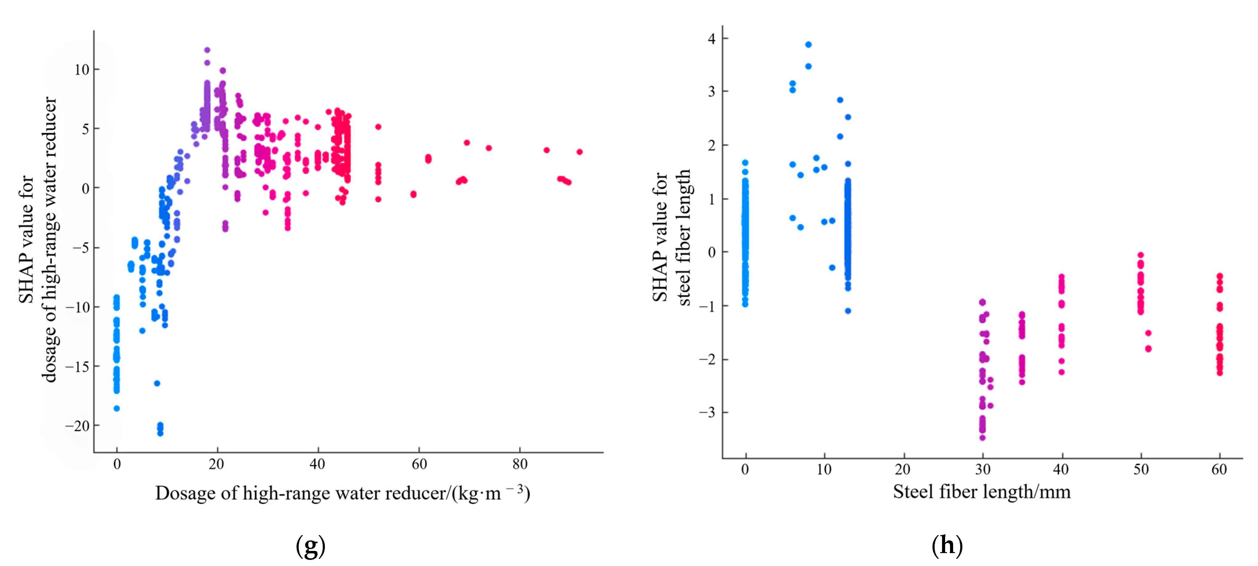
• Feature Importance Analysis: The SHAP value analysis results based on a wide range of experimental samples are consistent with the conclusions obtained from the experiments. Among the 14 input features, cement content, coarse aggregate content, and curing age are the most important factors affecting the compressive strength of concrete. For steel fiber reinforced concrete, in addition to the above three, an increase in steel fiber content, silicon powder content, dosage of high-range water reducer, and other parameter values has a positive impact on the compressive strength, providing useful guidance for the engineering design of concrete materials.
• The influence mechanism of steel fiber parameters: For steel fiber reinforced concrete, both local and global interpretation analysis based on SHAP shows that within an appropriate range, an increase in steel fiber content leads to an enhancement in the compressive strength of concrete, although the improvement is relatively small. The overall impact of steel fiber length on compressive strength is limited, but excessively long fiber has a negative effect. This is consistent with engineering practice, as overly long fibers can impair the workability of the mixture and the quality of construction.

Although this study confirms the effectiveness of a DNN framework integrated with the SHAP interpretability method in predicting the compressive strength of SFRC, several limitations remain. As a typical multiphase composite material, concrete has been extensively studied with respect to its strength properties. While this work investigates the influence of multiple features on the compressive strength of SFRC, the synergistic effects among these features have not yet been quantified. A deeper exploration of feature interdependencies may lead to the development of a more comprehensive and accurate strength prediction model. In addition, given the wide variety of deep learning architectures available today, adopting more advanced and powerful models may further improve prediction accuracy and interpretability, thereby offering more reliable guidance for engineering applications.

References

1. Zhao, Y.R.; Su, S.; Xie, Y.P.; Shi, J.N. Influence of Steel Fiber on the Flexural Toughness and Fatigue Damage of Reinforced Concrete Beam. Bull. Chin. Ceram. Soc. 2018, 37, 260–266. [Google Scholar]
2. Tanash, A.O.; Abu Bakar, B.; Muthusamy, K.; AL Biajawi, M.I. Effect of elevated temperature on mechanical properties of normal strength concrete: An overview. Mater. Today Proc. 2024, 107, 152–157. [Google Scholar]
3. Zhang, P.; Wang, C.; Gao, Z.; Wang, F. A review on fracture properties of steel fiber reinforced concrete. J. Build. Eng. 2023, 67, 105975. [Google Scholar] [CrossRef]
4. Ge, K.; Guo, Y.T.; Wang, C.; Hu, Z.Z. AI-based prediction of seismic time-history responses of RC frame structures considering varied structural parameters. J. Build. Eng. 2025, 106, 112643. [Google Scholar] [CrossRef]
5. Han, J.; Zhao, M.; Chen, J.; Lan, X. Effects of steel fiber length and coarse aggregate maximum size on mechanical properties of steel fiber reinforced concrete. Constr. Build. Mater. 2019, 209, 577–591. [Google Scholar] [CrossRef]
6. Fan, J.; Wang, C.; Song, L. Research and application of intelligent computation in civil engineering. J. Build. Struct. 2022, 43, 1–22. [Google Scholar]
7. Shafighfard, T.; Bagherzadeh, F.; Rizi, R.A.; Yoo, D.-Y. Data-driven compressive strength prediction of steel fiber reinforced concrete (SFRC) subjected to elevated temperatures using stacked machine learning algorithms. J. Mater. Res. Technol. 2022, 21, 3777–3794. [Google Scholar] [CrossRef]
8. Zhang, X.; Akber, M.Z.; Zheng, W. Prediction of seven-day compressive strength of field concrete. Constr. Build. Mater. 2021, 305, 124604. [Google Scholar] [CrossRef]
9. Li, Y.; Zhang, Q.; Kamiński, P.; Deifalla, A.F.; Sufian, M.; Dyczko, A.; Ben Kahla, N.; Atig, M. Compressive Strength of Steel Fiber-Reinforced Concrete Employing Supervised Machine Learning Techniques. Materials 2022, 15, 4209. [Google Scholar] [CrossRef] [PubMed]
10. Rudin, C. Stop explaining black box machine learning models for high stakes decisions and use interpretable models instead. Nat. Mach. Intell. 2019, 1, 206–215. [Google Scholar] [CrossRef] [PubMed]
11. Lundberg, S.M.; Lee, S.I. A unified approach to interpreting model predictions. In Proceedings of the 31st International Conference on Neural Information Processing Systems, Long Beach, CA, USA, 4–9 December 2017; Curran Associates Inc.: Red Hook, NY, USA, 2017; pp. 4768–4777. [Google Scholar]
12. Sarker, I.H. Deep Learning: A Comprehensive Overview on Techniques, Taxonomy, Applications and Research Directions. SN Comput. Sci. 2021, 2, 420. [Google Scholar] [CrossRef] [PubMed]
13. An, P.; Cao, D.P.; Zhao, B.Y.; Yang, X.L.; Zhang, M. Reservoir physical parameters prediction based on LSTM recurrent neural network. Prog. Geophys. 2019, 34, 1849–1858. [Google Scholar]
14. Snoek, J.; Larochelle, H.; Adams, R.P. Practical Bayesian Optimization of Machine Learning Algorithms. Adv. Neural Inf. Process. Syst. 2012, 25, 2951–2959. [Google Scholar]
15. Hu, W.H.; Xu, Z.M.; Liu, Q.; Lu, W.; Teng, J. Study on internal force variation law of transfer truss and joint of a super high-rise building based on multi-scale finite element model modification by monitoring data. J. Build. Struct. 2023, 44, 236–246. [Google Scholar]
16. Key Material Properties of Ultra-High Performance Concrete (UHPC)-Mendeley Data[EB/OL]. Available online: https://daks.uni-kassel.de/entities/dataset/ff37a8c0-aa9e-4b0c-ab4c-905c3ebbe797 (accessed on 6 September 2023).
17. Mahjoubi, S.; Meng, W.; Bao, Y. Auto-tune learning framework for prediction of flowability, mechanical properties, and porosity of ultra-high-performance concrete (UHPC). Appl. Soft Comput. 2022, 115, 108182. [Google Scholar] [CrossRef]
18. Atiş, C.D.; Karahan, O. Properties of steel fiber reinforced fly ash concrete. Constr. Build. Mater. 2009, 23, 392–399. [Google Scholar] [CrossRef]
19. Dai, L.; Wu, X.; Zhou, M.; Ahmad, W.; Ali, M.; Sabri, M.M.S.; Salmi, A.; Ewais, D.Y.Z. Using Machine Learning Algorithms to Estimate the Compressive Property of High Strength Fiber Reinforced Concrete. Materials 2022, 15, 4450. [Google Scholar] [CrossRef] [PubMed]
20. Zhao, G.F.; Huang, C.K. Performance and application of steel fiber reinforced concrete. Ind. Constr. 1989, 2–9. [Google Scholar]
21. Soroush, M.; Yi, B. The Key Material Properties of Ultra-High-Performance Concrete (UHPC). Mendeley Data 2021. Available online: https://data.mendeley.com/datasets/dd62d5hyzr/1 (accessed on 6 September 2023).
22. Feng, D.; Wu, G. Interpretable machine learning-based modeling approach for fundamental properties of concrete structures. J. Build. Struct. 2022, 43, 228–238. [Google Scholar]
23. GB 50010-2010; Code for Design of Concrete Structures. China Standard Press: Beijing, China, 2010.
24. ACI 544.4R-18; Guide to Design with Fiber-Reinforced Concrete. American Concrete Institute: Farmington Hills, MI, USA, 2018.
25. CEB-FIP Model Code 1990; Comite Euro-lnternational Du Beton. Thomas Telford Publishing: London, UK, 1993.
Figure 1. Schematic diagram of the basic framework of fully connected neural networks.
Applsci 15 06848 g001
Figure 2. Schematic representation of the SHAP additive interpretation.
Applsci 15 06848 g002
Figure 3. The performance of four kinds of models on the training and testing sets: (a) DNN model; (b) RF model; (c) XGB model; (d) BP model.
Applsci 15 06848 g003
Figure 4. The performance of four kinds of models on the training and testing sets: (a) DNN model; (b) GB 50010 model; (c) ACI 544.4R model; (d) CEB-FIP model.
Applsci 15 06848 g004
Figure 5. Force plot of samples by SHAP: (a) sample 1; (b) sample 2; (c) sample3.
Applsci 15 06848 g005
Figure 6. SHAP summary plot.
Applsci 15 06848 g006
Figure 7. Feature dependence plots by SHAP: (a) SHAP value for cement content; (b) SHAP value for age; (c) SHAP value for steel fiber content; (d) SHAP value for silicon powder content; (e) SHAP value for sand content; (f) SHAP value for water content; (g) SHAP value for dosage of high-range water reducer; (h) SHAP value for steel fiber length.
Applsci 15 06848 g007aApplsci 15 06848 g007b