1. Introduction
6D pose estimation is a highly complex problem in computer vision. It involves predicting the position and orientation of 3D objects in space, which requires determining both rotational and translational information for the target object. Typically, this process involves localizing objects using object detection or semantic segmentation before estimating their pose. As a critical concept in computer vision, 6D pose estimation plays a vital role in various applications, including robotic grasping [
1,
2], autonomous driving [
3,
4], and augmented reality [
5].
Traditional methods for pose estimation [
1,
6,
7] rely on handcrafted features to establish 2D–3D correspondences between images and 3D object meshes. However, these methods face significant challenges, such as sensor noise, variable lighting conditions, and visual ambiguity. Recent approaches leverage deep learning, using convolutional neural networks (CNNs) or Transformer-based architectures [
8] on RGB images to address these challenges. These methods typically provide pixel-level correspondences [
9,
10,
11,
12] or predict the 2D image locations of predefined 3D keypoints [
13,
14], yielding more robust results. Despite these advances, challenges, such as handling textureless objects and severe occlusions, remain unresolved.
To address the challenges of 6D pose estimation and leveraging the decreasing cost of RGB-D sensors, recent studies (e.g., PVN3D [
15], FFB6D [
16], RCVPose [
17], and DFTr [
18]) have adopted RGB-D images for 6DoF object pose estimation. Given the large output space of 6DoF, existing RGB-D-based methods predict predefined 3D keypoints in space (i.e., establishing sparse 3D–3D correspondences) and then solve for the pose using least-squares fitting. While these sparse keypoint approaches provide fundamental cues for object pose estimation, they still have several limitations. First, they often involve time-consuming procedures, such as keypoint voting. Second, predicting occluded keypoints remains challenging. Third, they may fail to locate object landmarks under viewpoint changes [
19].
Another approach in RGB-D methods aims to directly predict object poses from feature representations generated by neural networks, such as DenseFusion [
20] and ES 6D [
21]. Uni 6D [
22] and Uni 6Dv2 [
23] further integrate RGB and depth feature extraction for direct pose prediction. While these methods bypass the need for explicit 2D–3D correspondence, the pose derivation process is less interpretable, since object poses are regressed directly from feature embeddings. Consequently, object poses estimated using direct pose estimation methods are often less accurate. This weakness has also been observed in related research, such as camera pose estimation (also known as ego-motion estimation) [
24,
25]. The reasons for the inaccuracy of pose regression methods are elaborated in [
26].
To address the limitations of existing RGB-D methods, we propose a novel keypoint cloud extraction method. This method replaces the target point cloud with keypoint cloud to mitigate the impact of redundant information, thereby alleviating the drawbacks of sparse correspondences and pose regression. Our approach involves using dense 2D–3D correspondences, leveraging the RGB channel, and 3D–3D correspondences, utilizing the D channel input to establish correspondences with the 3D object model’s point cloud. To better integrate RGB and depth information, we have modified the G2L-Net method [
27].
We detect 2D edge information in RGB images using the Sobel edge detection operator and derive point cloud edge keypoints through semantic segmentation masks and 3D–3D correspondences. Additionally, we compute the curvature matrix from the depth map and use a first-order differential Sobel operator combined with masks to supplement point cloud internal keypoint information. The resulting keypoint cloud is fed into an improved pose estimation network, which maintains interpretability and achieves higher accuracy than sparse correspondence methods.
Furthermore, to accelerate the convergence of the pose estimation network, we employ keypoint cloud and residual structures. This approach is more efficient than time-consuming processes like PnP-RANSAC. Our method not only enhances the accuracy of pose estimation but also improves the efficiency of the network’s convergence.
This paper makes the following key contributions:
We propose a novel keypoint cloud extraction algorithm called RSCS, which integrates RGB images and depth images to extract 3D keypoint cloud from both edge information and depth information. This approach effectively reduces redundancy and enhances the quality of correspondences for pose estimation.
Building on the G2L-Net method [
27], we introduce RSCS6D, which leverages semantic segmentation via PIDNet [
28] and the keypoints extracted by RSCS. By incorporating these keypoints into an improved pose estimation network, we achieve more accurate 6D pose predictions.
To meet the diverse needs of industrial applications, this paper presents a lightweight version of RSCS6D, namely RSCS6D_Pruned. Considering the feature redundancy in the pose estimation network of RSCS6D, we utilize a coarse-grained pruning algorithm, Network Slimming (NS) pruning [
29], to optimize the network and reduce model complexity and computational cost.
Our method improves the accuracy of pose estimation while accelerating network convergence through the use of keypoint cloud and residual structures. Additionally, unlike direct pose regression methods, our approach retains a high level of interpretability, making it easier to understand and debug. These contributions provide a robust solution for 6D pose estimation from RGB-D images. The overview of our method is illustrated in
Figure 1.
Furthermore, we introduce a lightweight version of our method to meet the needs of various industrial applications. This lightweight version inherits the advantages of the original method while reducing computational complexity and resource requirements.
3. Proposed Method
Given an RGB-D image, the task of 6DoF pose estimation is to determine the rigid transformation that maps an object from its world coordinate system to the camera coordinate system. This transformation is composed of a 3D rotation matrix and a translation vector .
3.1. Overview
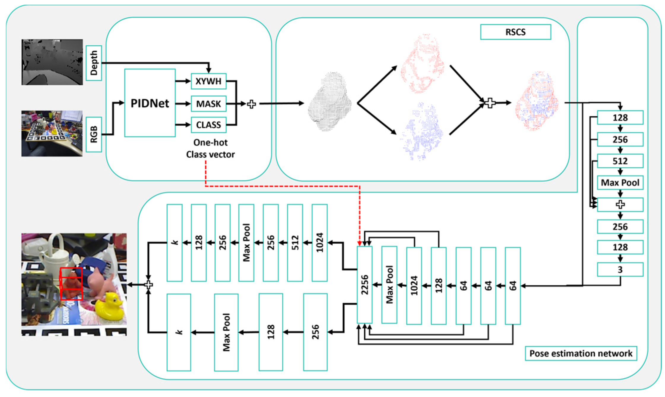
To address the problem of 6D pose estimation from RGB-D images, we propose RSCS6D, a keypoint extraction-based method that includes the RSCS keypoint extraction algorithm, as shown in
Figure 2. Specifically, we first obtain the mask of the RGB image using a semantic segmentation algorithm (PIDNet in this work) and combine it with the depth map to acquire the point cloud of the target object.
The RSCS keypoint extraction algorithm extracts keypoints from the point cloud in two steps:
Edge Keypoint Extraction: Convert the RGB image to grayscale and use the Sobel edge detection operator to identify 2D edge keypoints. These are then combined with the depth map to derive the point cloud edge keypoints.
Internal Keypoint Extraction: Compute the curvature matrix from the depth map using PCA-based plane fitting and apply the Sobel operator to the curvature matrix to identify keypoints with significant curvature changes.
The union of these two sets of keypoints forms the final keypoint cloud. These keypoints are fed into a CNN-based pose estimation network to predict the translation of the target object. Finally, a 3D tight bounding box is generated from the keypoint cloud, and the Kabsch algorithm is used to predict the rotation of the target object. This approach maintains interpretability while achieving higher accuracy and faster convergence compared to traditional methods.
3.2. Obtaining Target Point Cloud
In practical scenarios involving viewpoint changes, varying lighting conditions, and background interference, the accuracy of point cloud extraction using only 2D bounding boxes from object detection algorithms is significantly reduced. To address this issue, pixel-level object classification through semantic segmentation algorithms is essential. In this work, we employ the PIDNet semantic segmentation algorithm, which not only effectively classifies 2D pixels but also performs pixel-level segmentation of 3D point clouds. This approach ensures robust and accurate point cloud extraction even under challenging conditions.
Inspired by the proportional-integral-derivative (PID) controller in dynamic systems, the PIDNet algorithm employs a tri-branch network design, consisting of proportional (P), integral (I), and derivative (D) branches. These branches, respectively, capture detailed information, contextual information, and boundary information from RGB images.
The integral branch gathers rich contextual information, which is fully integrated with boundary information. Additionally, the Pag module selectively combines this information with detailed information, ensuring that significant semantic features are not overshadowed. Boundary attention guides the Bag module to organically integrate these three types of information, forming fused features. Finally, multi-scale feature extraction from these fused features, by combining feature maps of different sizes, enhances the capture of spatial semantic information across scales, thereby improving the effectiveness of semantic segmentation.
The PIDNet-S version was chosen for its impressive performance on the Cityscapes dataset, achieving a speed of 93.2 FPS and an accuracy of 78.6% mIOU. This balance of speed and accuracy makes it suitable for practical applications. To further enhance the accuracy of 2D segmentation and optimize the final 6D pose estimation results, several methods can be employed. These include utilizing keypoint cloud to improve the accuracy of 3D point clouds and pruning the network structure to eliminate redundant computations in feature extraction. These approaches aim to enhance the overall efficiency and effectiveness of the segmentation and pose estimation process.
The mask image obtained from semantic segmentation provides 2D point-wise labels, indicating the location information of the target object. By combining this mask with depth information from the same pixels, we can derive the 3D point cloud coordinates of the target object. This integration of 2D labels and depth data allows for the conversion of 2D image information into 3D spatial coordinates, effectively reconstructing the target object’s shape and position in 3D space.
The conversion from image coordinates to camera coordinates can be expressed in matrix form as follows:
Here, (x, y, z) represents the coordinates of a point in the camera coordinate system, (u, v) are the coordinates in the image plane, D is the depth information at pixel (u, v), and f is the focal length of the camera. This matrix formulation allows for the transformation of 2D image points into 3D camera coordinates using depth information.
3.3. Keypoint Cloud Extraction
In the field of pose estimation, relying solely on image-based detection is insufficient for obtaining the 3D information for target objects. On the other hand, point cloud data, though rich in 3D information, are challenging to process due to their sparse, irregular, and unordered nature. To address these challenges, a hybrid approach that leverages the strengths of both image and point cloud data is often adopted by researchers.
There is a subtle relationship between images and point clouds: the projection of 3D keypoint cloud onto a 2D image plane typically corresponds to the edges of the target object. This allows for the conversion of 2D images to 3D point clouds through coordinate system transformation. To further enhance the internal feature information of point clouds, the neighborhood relationships in 2D images can be utilized to define neighborhood relationships in 3D space. By selecting keypoints based on the curvature of point cloud neighbors, the extraction of internal keypoints within the point cloud can be improved.
Based on this understanding, we propose a novel keypoint cloud extraction algorithm that combines edge detection and differential curvature analysis. This approach aims to effectively extract keypoints from point clouds, addressing the limitations of using either image or point cloud information alone.
3.3.1. Sobel Operator
The Sobel operator, a 3 × 3 kernel, consists of two sub-operators for horizontal and vertical directions. It detects edges by calculating the brightness differential in both directions at the target pixel. Let (x, y) denote the coordinates of a pixel in an image, and
f (
x,
y) represent the grayscale value at that pixel. The mathematical expressions for the horizontal (
Gx) and vertical (
Gy) components are shown in Equations (3) and (4), and their matrix forms are illustrated in Equations (5) and (6).
In Equations (5) and (6), the symbol ∗ denotes the convolution operation. The matrices in these equations represent gradient templates used to compute the horizontal and vertical components of the image gradient. Here, F is the matrix of grayscale values from the neighborhood of the pixel point (x, y).
In this paper, we opted for the Sobel operator for edge detection due to its high computational efficiency and ease of implementation, particularly effective in images with distinct edges and clear textures, aligning well with our application scenario. While we considered other edge detection algorithms such as the Prewitt operator, Canny operator, and LoG (Laplacian of Gaussian) operator, these often yield fewer keypoints despite higher precision in certain aspects. Experiments with Sobel operators of different scales (e.g., 5 × 5, 7 × 7) revealed that larger scales, though more robust to noise, further reduce the number of keypoints.
Our pose estimation algorithm relies heavily on the quantity of keypoints, as a sufficient number provides richer information for subsequent pose estimation, enhancing measurement accuracy and reliability. Thus, our keypoint extraction algorithm aims to ensure an adequate number of feature points rather than solely pursuing extraction precision. We chose the Sobel operator and optimized its performance by adjusting parameters and integrating strategies like differential curvature calculation to better fit our pose estimation framework.
3.3.2. RS Algorithm for Edge Keypoint Extraction
The specific process of the target edge point cloud keypoint extraction algorithm is illustrated in
Figure 2 and consists of the following steps:
Process the RGB image using the PIDNet semantic segmentation algorithm to achieve pixel-level segmentation of the target object.
- 2.
2D Edge Detection:
Apply the Sobel edge detection operator to extract 2D edges of the target object and refine them using the segmentation results. This ensures the detected edges accurately correspond to the target object.
- 3.
3D Transformation:
Combine the camera intrinsic matrix and depth map to obtain depth information. Using Equation (2), transform the 2D edge keypoints into 3D point cloud edge keypoints, thereby completing the extraction of edge keypoints from the point cloud.
This three-step process effectively extracts edge keypoints from the point cloud, ensuring accuracy and relevance to the target object.
3.3.3. Curvature Calculation Using 2D Neighborhood-Based PCA
Traditional point cloud PCA plane fitting methods [
38] often use nearest-neighbor algorithms to determine the neighborhood points of a target point. This paper presents a method for curvature calculation in 3D point clouds using 2D neighborhood-based PCA. The process involves extracting an 8-neighborhood pixel matrix from the RGB image, standardizing it, and computing its covariance matrix. Singular Value Decomposition (SVD) is then applied to obtain singular values, which are used to calculate the curvature of the target point. This approach leverages 2D neighborhood relationships and depth information to enhance the accuracy and efficiency of curvature calculation in 3D point clouds. It addresses limitations of traditional nearest-neighbor methods by providing a more accurate representation of local geometric structure and improving plane fitting reliability. The specific steps are shown in Algorithm 1.
| Algorithm 1. Curvature Calculation Using 2D Neighborhood-Based PCA |
Input: RGB-D Data
Output: Curvature Value of Target Points
|
| Extract 8-Neighbor Pixel Matrix: Extract the 8-neighborhood pixel matrix X2D of the target point in the RGB image space. Using the camera intrinsic parameters and depth map, construct the corresponding 3D point cloud neighborhood matrix X3D. Standardization: Standardize the matrix X3D to ensure numerical stability and consistency in scale. Covariance and SVD Decomposition: Compute the covariance matrix H of the standardized matrix and perform Singular Value Decomposition (SVD). where Curvature Calculation: Calculate the curvature value of the target point using the singular values obtained from the SVD decomposition.
|
This method leverages 2D neighborhood relationships and depth information to enhance the accuracy and efficiency of curvature calculation in 3D point clouds. However, potential failure modes, such as segmentation errors, sensor noise, and missing depth values, can adversely affect the determination of neighborhood points and subsequent curvature calculations, thereby reducing the accuracy and stability of keypoint extraction. To address this, the paper proposes an improved strategy: using only keypoints with valid depth values and treating each target’s 1000 keypoints as a whole. By randomly selecting different combinations of keypoints in each computation round and iterating multiple times, the impact of segmentation errors, sensor noise, and missing depth values on keypoint extraction accuracy is effectively mitigated. This significantly enhances the robustness of keypoint extraction and the overall performance of pose estimation.
3.3.4. CS Algorithm for Internal Keypoint Extraction
Curvature is a critical feature for describing the concavity or convexity of a surface, reflecting the degree of variation in the point cloud surface. Points with high curvature values, indicating significant surface changes, are often considered key points in 3D point clouds.
In this work, we calculate the curvature of points in a 3D point cloud by leveraging 2D neighborhood relationships from RGB images. The process involves the following steps:
Using PIDNet algorithm, we obtain the matrix
Cobj, which consists of the coordinates of the target object in the 2D image coordinate system:
- 2.
Calculate 2D Bounding Box Parameters:
From matrix
Cobj, we compute the parameters of the 2D bounding box (x, y, w, h) using the following formulas:
- 3.
Generate 2D Coordinate Matrix and Label Vector:
Using the bounding box parameters, we generate the 2×wh 2D coordinate matrix
Cbbx:
Simultaneously, we obtain the corresponding label vector
Lobj:
Here, represents the pixel mask value at coordinate position .
- 4.
Calculate 3D Coordinate Matrix:
Combining the depth map with the camera model (Equation (2)), we compute the 3D coordinate matrix
PCbbx.
For convenience,
PCbbx can be represented as column vectors:
- 5.
Curvature Calculation:
For each point
in
PCbbx, we use Algorithm 1 to compute the curvature
. These curvature values form the curvature matrix
Q:
- 6.
Curvature Gradient Matrix:
Using the Sobel operator, we process the curvature matrix
Q to obtain the curvature gradient matrix
GQ:
- 7.
Key Point Selection:
By setting a specific threshold
T and combining it with the curvature gradient matrix
GQ, we obtain the curvature label vector
LQ:
Combining
LQ with the target label vector
Lobj using a logical AND operation, we screen out the key points in the point cloud:
Finally, we obtain the point cloud key points matrix
PCkey:
where
is the
j-th column of matrix
PCbbx,
, and
T is the threshold for the curvature gradient matrix. The label vector
Lkey is used to determine whether a point is a key point in the point cloud.
After generating the curvature matrix for the point cloud, we apply a first-order differential operator to detect points with significant curvature changes. By selecting an appropriate threshold, we identify these high-curvature points as key points. Finally, combining these 2D key points with depth information and camera intrinsics, we transform them into 3D space to obtain the key point cloud.
This method effectively identifies critical points in the point cloud, enhancing the accuracy and robustness of subsequent pose estimation tasks.
3.4. 6D Pose Estimation Network
After extracting keypoint cloud using the RSCS algorithm, we construct a network for pose estimation. Inspired by ResNet and G2L-Net, the RSCS6D algorithm incorporates a translational residual to accelerate network convergence. Specifically, we design a network that predicts the translation by estimating the deviation between the predicted translation and the object’s center. This residual helps refine the translation prediction.
To address the limitations of global point features and inspired by G2L-Net, RSCS6D defines a point cloud key vector cluster to capture viewpoint information. We also design a rotation prediction network and a rotation residual prediction network based on keypoint cloud to extract features and predict rotation and residual information.
Finally, the RSCS6D algorithm uses the Kabsch algorithm, combined with the eight vertices of the ground-truth 3D tight bounding box, to compute the predicted rotation matrix. This comprehensive approach ensures accurate and efficient pose estimation.
The training process of the RSCS6D algorithm is divided into two main components: global localization and pose estimation.
This component involves obtaining pixel-wise labels of the target object using a semantic segmentation algorithm. In this work, we employ the PIDNet algorithm [
28], though other advanced methods can also be used.
- 2.
Pose Estimation:
The input to this component is the keypoint cloud extracted using the RSCS algorithm. The process begins with translation prediction, which estimates the deviation between the predicted translation and the object’s center. This residual is then used to refine the translation prediction by combining it with the predicted object center during the detection phase.
For rotation prediction, the network consists of three modules:
Key Vector Cluster Module: Predicts unit vectors pointing to keypoints. The loss function is the mean squared error (MSE) between the predicted and ground-truth direction vectors.
Rotation Prediction Module: Integrates point-wise embedding features to predict the object’s rotation. The predicted tight bounding box data from this module is compared with the ground-truth data using the Kabsch algorithm to estimate the point cloud rotation. The loss function is the MSE between the predicted and ground-truth tight bounding box data.
Rotation Residual Prediction Module: Inspired by the residual structure in ResNet, this module estimates the residual between the predicted and ground-truth rotations. It leverages point cloud key vector clusters to improve efficiency and reduce computational overhead.
This structured approach ensures accurate and efficient 6D pose estimation by combining semantic segmentation, keypoint extraction, and residual learning.
The RSCS6D pose estimation network draws inspiration from G2L-Net but features two fundamental differences. First, to address the issue of poor point cloud segmentation by traditional object detection algorithms, especially when objects are occluded, RSCS6D employs the semantic segmentation algorithm PIDNet to mitigate the impact of occlusion. Additionally, it leverages pixel-level two-dimensional segmentation results to perform three-dimensional pixel-level segmentation on the local scene point clouds (i.e., coarse point clouds), thereby obtaining the target key point clouds. Second, to tackle the problem of redundant information in traditional pose estimation algorithms that use coarse point clouds, RSCS6D precisely extracts key points from the coarse point clouds. This approach effectively reduces information redundancy, suppresses noise interference, accelerates network convergence, and enhances the efficiency and accuracy of pose estimation.
3.5. RSCS6D_Pruned: A Lightweight Version
In practical applications of 6D pose estimation algorithms, it is highly desirable for the algorithm to operate efficiently on platforms with limited computational resources. To broaden the applicability of the algorithm without compromising its original speed and accuracy, it is essential to minimize both the model’s parameter count and computational demands. However, the network architecture of the RSCS6D algorithm, which relies on concatenating feature maps from different stages to capture diverse feature information, presents a challenge. This concatenation operation leads to a substantial increase in the number of channels, with some channels expanding to counts of 2240 and even 2256. Such a large number of channels results in frequent feature reuse during convolution operations, indicating a high level of redundancy. This redundancy not only increases the computational load but also may affect the overall efficiency and performance of the algorithm on resource-constrained devices.
3.5.1. Network Slimming Pruning
NS (Network Slimming) pruning is a classic filter–level pruning method. It reduces model complexity and computation by cutting channels in layers with high channel numbers. In CNNs, convolutional layers are often structured as “convolution + BN + activation function”. NS pruning uses the scale factors of BN layers to measure channels for pruning.
Set
zin and
zout as the input and output of the BN layer, and
B as the current batch. The calculation formula for BN layer is as follows:
where
μB and
σB are the mean and variance of activations, and
ε is a small positive number to prevent division by zero.
The formula for calculating
zout is given by Equation (19):
Here, γ and β are trainable affine transformation parameters. Specifically, γ acts as a scale factor and β as a shift factor. This allows the network to adaptively adjust the distribution of the normalized features. The γ parameter controls the scaling of the normalized activation values, while β provides the shifting capability. This design enables the network to flexibly adjust feature distributions. It retains the benefits of normalization while avoiding excessive constraints on feature distribution, thereby enhancing the network’s flexibility and adaptability.
NS pruning introduces a scale factor
γ for each convolutional layer using BN. It applies
L1 regularization to
γ, encouraging sparsity in the convolutional kernels during training. The training loss function is Equation (20):
This loss function has two parts: the training loss and the regularization term. (x, y) are input data and target labels, and W represents trainable weights. The first term is the standard CNN training loss, while the second term λ∑g(γ) is an L1 regularization term on γ. λ is a penalty coefficient controlling the sparsity level. In experiments, g(γ) = ∣γ∣ because L1 regularization is effective for parameter sparsity and widely used in model compression.
3.5.2. Network Slimming Pruning for RSCS
Figure 3 compares the network architectures before and after pruning. The original structure in
Figure 3a uses a full-feature-map overlay fusion strategy, expanding the point cloud keypoint feature channels to 2256 dimensions. While this design enhances feature representation, it also significantly increases computational demands. The optimized structure in
Figure 3b employs NS pruning with a 50% pruning rate. This reduces the maximum feature channels from 2256 to 1077, while maintaining algorithm performance and improving computational efficiency.
NS pruning adaptively reduces channels based on task needs. It decreases model parameters and computation significantly. However, retraining is needed to restore pre-pruning accuracy. By integrating a lightweight pose estimation algorithm based on point cloud keypoints, a compact network can be built. This network has few parameters, low memory usage, and broad applicability.
4. Experiments
In this section, we present the experimental results of our RSCS6D method and compare it with other state-of-the-art approaches.
4.1. Implementation Details
To evaluate the performance of our point cloud keypoint-based pose estimation algorithm, experiments were conducted on the LineMod dataset. The hardware platform used includes a Windows 11 operating system and an NVIDIA GeForce RTX 4090 GPU with 24 GB of VRAM. Our framework was implemented using PyTorch 2.2.2. All experiments were performed on an Intel i9-14900K 3.60 GHz CPU and an NVIDIA GeForce RTX 4090 GPU.
We fine-tuned the PIDNet architecture [
28], which was pre-trained on ImageNet [
39], to obtain mask images for different categories of target objects. Point cloud keypoints were extracted from RGB-D data using the RSCS method and used for pose estimation. We then trained our improved pose estimation network based on G2L-Net [
27]. The network architecture is illustrated in
Figure 2.
In the experimental section, we indeed adjusted the network’s hyperparameters to optimize its performance and enhance the precision and efficiency of pose estimation. During this process, we referred to hyperparameter settings from other mature methods in related fields and made targeted adjustments based on the specific needs of our network architecture and task objectives.
For pose prediction, we used mean squared error (MSE) as the loss function, with units in millimeters. The Adam optimizer [
40] was employed to train the RSCS6D network. The initial learning rate was set to 0.001 and halved every 50 epochs, with a maximum of 200 epochs. This setup ensures efficient training and convergence of the network.
4.2. Dataset
The LineMod dataset [
41] comprises 15,783 images featuring 13 objects, each with approximately 1000 images. Most objects are textureless, and the dataset includes complex scenes with varying lighting conditions, posing significant challenges for pose estimation. Unlike the YCB dataset, which organizes data by scenes, LineMod is organized by objects. Each object’s folder contains depth maps, segmentation masks, RGB images, and text files with pose and annotation information, as well as camera intrinsics and depth scaling factors. LineMod focuses on single-object information; for example, the folder for the first object provides its segmentation masks, pose, and annotations, but not for other objects. Additionally, the dataset provides 3D models of the 13 objects in ply format.
4.3. Evaluation Metrics
In pose estimation tasks, the algorithm outputs a rotation matrix R and translation vector t, which describe the rigid transformation of the target object from the world coordinate system to the camera coordinate system. The accuracy of this transformation can be quantified using the Average Distance (ADD) metric, which measures the average Euclidean distance between the predicted and ground-truth positions of all 3D model points.
Given the ground-truth rotation matrix
R and translation vector
t, and the predicted rotation matrix
Rp and translation vector
tp, the ADD is calculated as follows:
Here:
M is the set of m 3D points of the object in the world coordinate system.
Rx + t represents the true position of a point in the camera coordinate system.
Rpx + tp represents the predicted position of the same point.
The ADD metric evaluates the precision of the pose estimation by averaging the Euclidean distances between the predicted and true positions of all model points. This provides a comprehensive measure of how well the estimated pose aligns with the ground truth.
For objects with symmetry, the ADD metric may not accurately reflect the performance of pose estimation algorithms, as symmetry can lead to multiple visually indistinct poses. To address this, DenseFusion introduced the ADD-S metric, which accounts for object symmetry by measuring the average minimum distance between transformed points in the predicted pose and the nearest points on the ground-truth model.
The ADD-S is calculated as follows:
The ADD-S metric addresses the limitations of ADD when evaluating symmetric objects by measuring the average minimum distance from transformed points in the predicted pose to the nearest points on the ground-truth model. Specifically, instead of calculating point-to-point distances, ADD-S computes the average of the minimum distances between each transformed point in the predicted pose and the closest point on the ground-truth model. If this average distance is less than 10% of the object’s diameter, the pose estimation is deemed correct.
4.4. Comparison with the State-of-the-Art Methods
The LineMOD dataset [
41] is a widely used benchmark for 6D object pose estimation, featuring 13 objects with significant shape variation. These objects are captured in sequences that include mild occlusions, cluttered backgrounds, textureless surfaces, and varying lighting conditions, making it challenging for accurate pose estimation in real-world scenarios.
Our approach follows the protocol established in previous works [
14,
20,
27,
42], which adopts a standard 15%/85% training/test split. This setup ensures a robust evaluation of pose estimation algorithms under diverse and realistic conditions.
Our proposed real-time pose estimation algorithm demonstrates superior performance on the LineMOD dataset, outperforming existing methods such as PVNet [
14], PoseCNN [
42], DenseFusion [
20], and G2L-Net [
27]. As shown in
Table 1, our algorithm achieves an average ADD accuracy of 99.32% across 13 objects, representing a 0.6% improvement over the best baseline method, G2L-Net (98.7%). Notably, our method sets new records for 11 objects, including ape and bench vise, with perfect ADD-S accuracy of 100% for symmetric objects like eggbox and glue.
In terms of real-time performance, our algorithm processes at 40 FPS, significantly surpassing DenseFusion (19 FPS) and G2L-Net (28 FPS). Importantly, these results are achieved without the need for refinement post-processing, leveraging the advantages of RGB-D data effectively.
4.5. Comparison of Different Pruning Rates
The lightweight pose estimation algorithm based on NS pruning with different pruning rates shows remarkable advantages on the LineMod dataset, as presented in
Table 2. All pruned versions (20–50%) maintain a high accuracy of over 99.3% while keeping the processing speed at 36–37 FPS, surpassing the baseline method. Notably, the 30%-pruned version achieves an average accuracy of 99.5% at 37 FPS with only 10.81 MB of parameters, setting a new benchmark for studies on ten objects including ape and bench vise. Moreover, on symmetric objects eggbox and glue, the ADD-S metric remains at 100%. These results highlight the algorithm’s significant improvements in accuracy, speed, and lightweight performance, with a considerable boost in overall effectiveness compared to traditional methods.
The NS pruning strategy shows excellent model compression ability. Although time increases slightly, the total parameters decrease and the average ADD improves, showing NS pruning’s strong model compression ability. The 30% pruned model offers the best balance, reducing parameters by 17.98% and raising ADD to 99.5% (+0.2%), while running at 37 FPS. The 50% pruned model, with 9.02 MB parameters (a 31.56% reduction), maintains 99.4% ADD, outperforming DenseFusion.
Considering accuracy, speed, and model size, the 30% pruned model is optimal. It achieves 99.5% ADD, an 84.24% parameter reduction to 10.81 MB, and a 39.29% speed boost (37 FPS), making it the final RSCS6D_Pruned algorithm. In summary, combining point cloud keypoint extraction with NS pruning enhances pose estimation in accuracy, speed, and model volume, offering a practical solution for real-time pose estimation in resource-constrained scenarios.
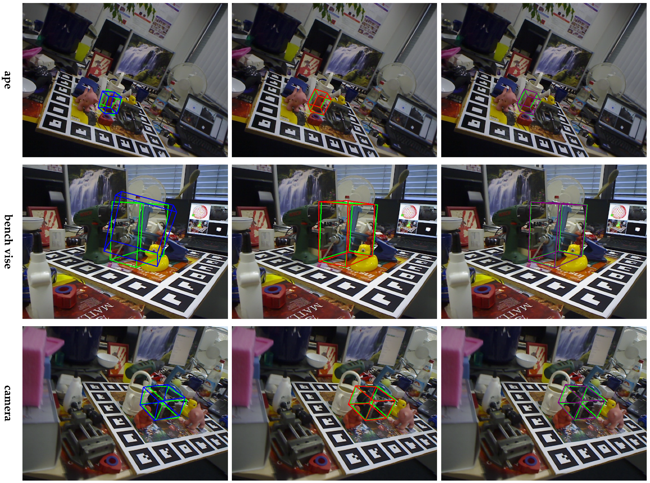
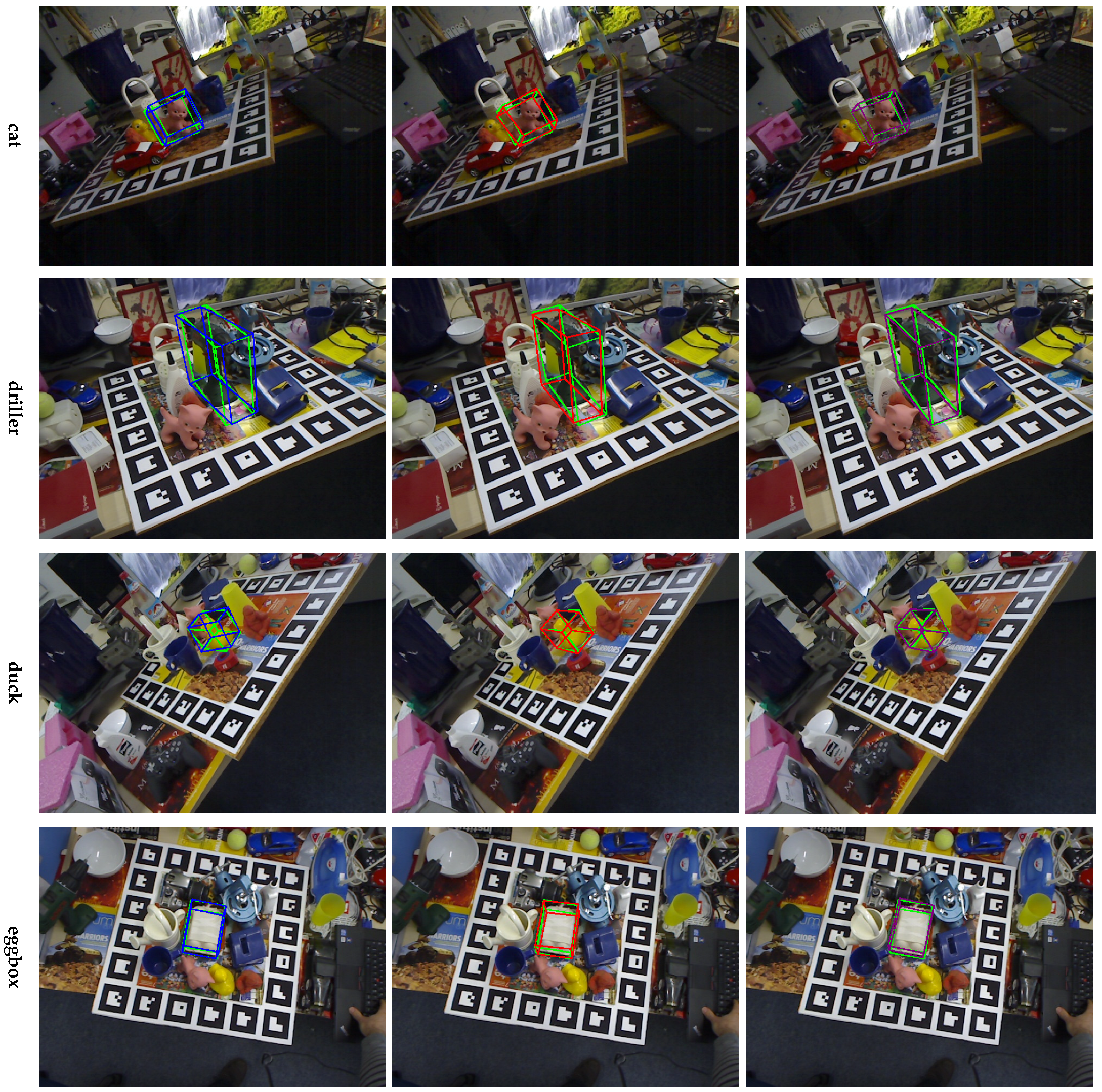
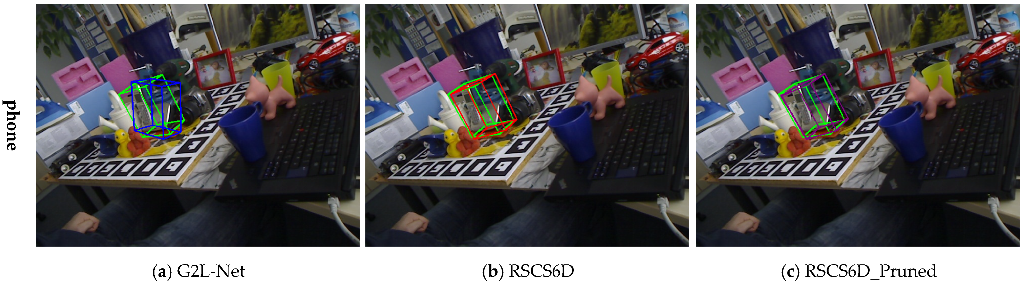
4.6. Visualization Results
In this study, 3D bounding-box visualization assesses various algorithms’ pose estimation performance. The process involves generating a reference bounding box from the target object’s 3D model, computing a predicted-pose bounding box using the algorithm-estimated rotation matrix and translation vector, and projecting it into 2D image space for comparison. On the LineMod dataset (
Figure 4,
Figure 5 and
Figure 6), green, blue, red, and purple boxes denote the ground-truth pose and predictions from G2L-Net, RSCS6D, and RSCS6D_Pruned algorithms. Results show our point-cloud-keypoint-based DL pose estimation algorithm outperforms the G2L-Net baseline. Both the original and quantized versions achieve higher positioning accuracy than the contrast algorithm, with the quantized version performing slightly better.
Quantitative analysis (
Table 1 and
Table 2) indicates that our algorithm and its quantized version significantly boost processing speed compared to G2L-Net. These findings, supported by visualization and quantitative results, confirm the effectiveness of our DL pose estimation method.
4.7. Limitations
Rigorous experiments validate that our method excels in real-time applications, responding quickly and maintaining high estimation accuracy across various complex scenarios. This demonstrates the potential of our keypoint-based approach to advance 6D pose estimation and to provide new insights and methods for related research and applications.
However, the performance of our algorithm is primarily constrained by the accuracy of the front-end semantic segmentation algorithm. Current depth cameras still have limitations in precision and stability, affecting the performance of the semantic segmentation module and, consequently, the pose estimation accuracy of the entire algorithm. Thus, while our algorithm optimizes pose estimation efficiency and accuracy to some extent, its performance is still limited by the front-end semantic segmentation algorithm and the performance of depth camera hardware.


