Abstract
In this work, we propose an improved network, RSCS6D, for 6D pose estimation from RGB-D images by extracting keypoint-based point clouds. Our key insight is that keypoint cloud can reduce data redundancy in 3D point clouds and accelerate the convergence of convolutional neural networks. First, we employ a semantic segmentation network on the RGB image to obtain mask images containing positional information and per-pixel labels. Next, we introduce a novel keypoint cloud extraction algorithm that combines RGB and depth images to detect 2D keypoints and convert them into 3D keypoints. Specifically, we convert the RGB image to grayscale and use the Sobel edge detection operator to identify 2D edge keypoints. Additionally, we compute the Curvature matrix from the depth image and apply the Sobel operator to extract keypoints critical for 6D pose estimation. Finally, the extracted 3D keypoint cloud is fed into the 6D pose estimation network to predict both translation and rotation.
1. Introduction
6D pose estimation is a highly complex problem in computer vision. It involves predicting the position and orientation of 3D objects in space, which requires determining both rotational and translational information for the target object. Typically, this process involves localizing objects using object detection or semantic segmentation before estimating their pose. As a critical concept in computer vision, 6D pose estimation plays a vital role in various applications, including robotic grasping [1,2], autonomous driving [3,4], and augmented reality [5].
Traditional methods for pose estimation [1,6,7] rely on handcrafted features to establish 2D–3D correspondences between images and 3D object meshes. However, these methods face significant challenges, such as sensor noise, variable lighting conditions, and visual ambiguity. Recent approaches leverage deep learning, using convolutional neural networks (CNNs) or Transformer-based architectures [8] on RGB images to address these challenges. These methods typically provide pixel-level correspondences [9,10,11,12] or predict the 2D image locations of predefined 3D keypoints [13,14], yielding more robust results. Despite these advances, challenges, such as handling textureless objects and severe occlusions, remain unresolved.
To address the challenges of 6D pose estimation and leveraging the decreasing cost of RGB-D sensors, recent studies (e.g., PVN3D [15], FFB6D [16], RCVPose [17], and DFTr [18]) have adopted RGB-D images for 6DoF object pose estimation. Given the large output space of 6DoF, existing RGB-D-based methods predict predefined 3D keypoints in space (i.e., establishing sparse 3D–3D correspondences) and then solve for the pose using least-squares fitting. While these sparse keypoint approaches provide fundamental cues for object pose estimation, they still have several limitations. First, they often involve time-consuming procedures, such as keypoint voting. Second, predicting occluded keypoints remains challenging. Third, they may fail to locate object landmarks under viewpoint changes [19].
Another approach in RGB-D methods aims to directly predict object poses from feature representations generated by neural networks, such as DenseFusion [20] and ES 6D [21]. Uni 6D [22] and Uni 6Dv2 [23] further integrate RGB and depth feature extraction for direct pose prediction. While these methods bypass the need for explicit 2D–3D correspondence, the pose derivation process is less interpretable, since object poses are regressed directly from feature embeddings. Consequently, object poses estimated using direct pose estimation methods are often less accurate. This weakness has also been observed in related research, such as camera pose estimation (also known as ego-motion estimation) [24,25]. The reasons for the inaccuracy of pose regression methods are elaborated in [26].
To address the limitations of existing RGB-D methods, we propose a novel keypoint cloud extraction method. This method replaces the target point cloud with keypoint cloud to mitigate the impact of redundant information, thereby alleviating the drawbacks of sparse correspondences and pose regression. Our approach involves using dense 2D–3D correspondences, leveraging the RGB channel, and 3D–3D correspondences, utilizing the D channel input to establish correspondences with the 3D object model’s point cloud. To better integrate RGB and depth information, we have modified the G2L-Net method [27].
We detect 2D edge information in RGB images using the Sobel edge detection operator and derive point cloud edge keypoints through semantic segmentation masks and 3D–3D correspondences. Additionally, we compute the curvature matrix from the depth map and use a first-order differential Sobel operator combined with masks to supplement point cloud internal keypoint information. The resulting keypoint cloud is fed into an improved pose estimation network, which maintains interpretability and achieves higher accuracy than sparse correspondence methods.
Furthermore, to accelerate the convergence of the pose estimation network, we employ keypoint cloud and residual structures. This approach is more efficient than time-consuming processes like PnP-RANSAC. Our method not only enhances the accuracy of pose estimation but also improves the efficiency of the network’s convergence.
This paper makes the following key contributions:
- RSCS Algorithm for Keypoint Cloud Extraction:
We propose a novel keypoint cloud extraction algorithm called RSCS, which integrates RGB images and depth images to extract 3D keypoint cloud from both edge information and depth information. This approach effectively reduces redundancy and enhances the quality of correspondences for pose estimation.
- RSCS6D Method for Pose Estimation:
Building on the G2L-Net method [27], we introduce RSCS6D, which leverages semantic segmentation via PIDNet [28] and the keypoints extracted by RSCS. By incorporating these keypoints into an improved pose estimation network, we achieve more accurate 6D pose predictions.
- RSCS6D_Pruned: A Lightweight Version:
To meet the diverse needs of industrial applications, this paper presents a lightweight version of RSCS6D, namely RSCS6D_Pruned. Considering the feature redundancy in the pose estimation network of RSCS6D, we utilize a coarse-grained pruning algorithm, Network Slimming (NS) pruning [29], to optimize the network and reduce model complexity and computational cost.
Our method improves the accuracy of pose estimation while accelerating network convergence through the use of keypoint cloud and residual structures. Additionally, unlike direct pose regression methods, our approach retains a high level of interpretability, making it easier to understand and debug. These contributions provide a robust solution for 6D pose estimation from RGB-D images. The overview of our method is illustrated in Figure 1.
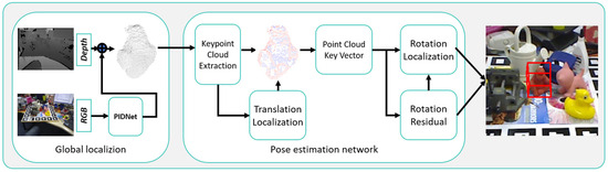
Figure 1.
The overview of RSCS6D.
Furthermore, we introduce a lightweight version of our method to meet the needs of various industrial applications. This lightweight version inherits the advantages of the original method while reducing computational complexity and resource requirements.
2. Materials and Methods
2.1. Direct Pose Estimation
Recent studies [20,21,22,23] have focused on directly predicting rotation and translation for pose estimation. DenseFusion [20] introduced a dense fusion module that fuses RGB and depth features at the pixel level to predict object poses, selecting the final pose based on the pixel with the highest confidence. ES6D [21] proposed XYZNet to reduce the demand for random memory access in dense fusion modules, enhancing time efficiency. It also introduced the A(M)GPD loss to address challenges posed by symmetric objects, improving upon the previous ADD-S loss. Experimental results demonstrated that the A(M)GPD loss is more effective for symmetric objects. Unit6D [22] and Unit6Dv2 [23] improved pose estimation by incorporating additional UV data as input to resolve projection factorization issues, enabling more accurate object pose estimation with a unified backbone.
While direct pose prediction (or regression) methods are time-efficient, they generally exhibit reduced performance compared to keypoint-based methods, particularly due to sensor noise.
2.2. Keypoint Extraction Techniques
2.2.1. Keypoint Extraction
Keypoint extraction in point clouds is crucial for pose estimation, point cloud registration, and 3D reconstruction, as it reduces data volume and enhances processing efficiency. The ISS algorithm [30] ensures rotational invariance by constructing covariance matrices to characterize local geometric distributions, performing robustly against density variations and noise. Harris-3D [31] extends 2D gradient analysis to 3D normal vector fields, though its cross-view stability hinges on normal estimation accuracy. SIFT-3D [32] builds a 3D Hessian matrix based on differential geometry for high repeatability, yet with high computational complexity. Engineering solutions, like clustering-curvature fusion [33] and cross-dimensional mapping systems [34], enable efficient feature extraction in specific scenarios, but balancing generalization capability and computational efficiency remains challenging. Developing dynamic feature detection frameworks adaptive to computing resources emerges as a promising research direction.
2.2.2. Keypoint-Based Pose Estimation
Unlike direct pose prediction methods, keypoint-based approaches [15,16,17,18] enhance robustness by leveraging projection equations. These methods define predetermined keypoints on the object’s surface and predict their locations in the image frame or camera coordinate system. The object’s pose is then computed based on these correspondences using PnP-RANSAC or least-squares fitting [35,36].
PVN3D [15] extends PVNet [14] to predict keypoints in 3D space, addressing the issue where small projection errors can lead to significant real-world deviations. FFB6D [16] further improves upon PVN3D [15] by incorporating a bidirectional fusion module to share information between the two modalities at an early stage. RCVPose [17] introduces a novel keypoint voting scheme using 1D radial voting to reduce cumulative errors in each channel, thereby significantly improving the accuracy of keypoint localization. DFTr [18] employs Transformer blocks to fuse cross-modal features and transmit global information between the two modalities. Additionally, DFTr [18] proposes a non-iterative weighted vector voting scheme to reduce computational costs, replacing the MeanShift [37] algorithm for keypoint voting.
Overall, keypoint-based methods offer greater robustness and accuracy compared to direct pose prediction methods, making them suitable for applications where precision is critical.
3. Proposed Method
Given an RGB-D image, the task of 6DoF pose estimation is to determine the rigid transformation that maps an object from its world coordinate system to the camera coordinate system. This transformation is composed of a 3D rotation matrix and a translation vector .
3.1. Overview
To address the problem of 6D pose estimation from RGB-D images, we propose RSCS6D, a keypoint extraction-based method that includes the RSCS keypoint extraction algorithm, as shown in Figure 2. Specifically, we first obtain the mask of the RGB image using a semantic segmentation algorithm (PIDNet in this work) and combine it with the depth map to acquire the point cloud of the target object.
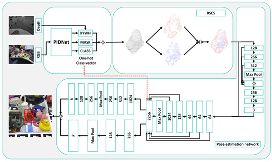
Figure 2.
The pipeline of RSCS6D.
The RSCS keypoint extraction algorithm extracts keypoints from the point cloud in two steps:
- Edge Keypoint Extraction: Convert the RGB image to grayscale and use the Sobel edge detection operator to identify 2D edge keypoints. These are then combined with the depth map to derive the point cloud edge keypoints.
- Internal Keypoint Extraction: Compute the curvature matrix from the depth map using PCA-based plane fitting and apply the Sobel operator to the curvature matrix to identify keypoints with significant curvature changes.
The union of these two sets of keypoints forms the final keypoint cloud. These keypoints are fed into a CNN-based pose estimation network to predict the translation of the target object. Finally, a 3D tight bounding box is generated from the keypoint cloud, and the Kabsch algorithm is used to predict the rotation of the target object. This approach maintains interpretability while achieving higher accuracy and faster convergence compared to traditional methods.
3.2. Obtaining Target Point Cloud
In practical scenarios involving viewpoint changes, varying lighting conditions, and background interference, the accuracy of point cloud extraction using only 2D bounding boxes from object detection algorithms is significantly reduced. To address this issue, pixel-level object classification through semantic segmentation algorithms is essential. In this work, we employ the PIDNet semantic segmentation algorithm, which not only effectively classifies 2D pixels but also performs pixel-level segmentation of 3D point clouds. This approach ensures robust and accurate point cloud extraction even under challenging conditions.
Inspired by the proportional-integral-derivative (PID) controller in dynamic systems, the PIDNet algorithm employs a tri-branch network design, consisting of proportional (P), integral (I), and derivative (D) branches. These branches, respectively, capture detailed information, contextual information, and boundary information from RGB images.
The integral branch gathers rich contextual information, which is fully integrated with boundary information. Additionally, the Pag module selectively combines this information with detailed information, ensuring that significant semantic features are not overshadowed. Boundary attention guides the Bag module to organically integrate these three types of information, forming fused features. Finally, multi-scale feature extraction from these fused features, by combining feature maps of different sizes, enhances the capture of spatial semantic information across scales, thereby improving the effectiveness of semantic segmentation.
The PIDNet-S version was chosen for its impressive performance on the Cityscapes dataset, achieving a speed of 93.2 FPS and an accuracy of 78.6% mIOU. This balance of speed and accuracy makes it suitable for practical applications. To further enhance the accuracy of 2D segmentation and optimize the final 6D pose estimation results, several methods can be employed. These include utilizing keypoint cloud to improve the accuracy of 3D point clouds and pruning the network structure to eliminate redundant computations in feature extraction. These approaches aim to enhance the overall efficiency and effectiveness of the segmentation and pose estimation process.
The mask image obtained from semantic segmentation provides 2D point-wise labels, indicating the location information of the target object. By combining this mask with depth information from the same pixels, we can derive the 3D point cloud coordinates of the target object. This integration of 2D labels and depth data allows for the conversion of 2D image information into 3D spatial coordinates, effectively reconstructing the target object’s shape and position in 3D space.
The conversion from image coordinates to camera coordinates can be expressed in matrix form as follows:
Here, (x, y, z) represents the coordinates of a point in the camera coordinate system, (u, v) are the coordinates in the image plane, D is the depth information at pixel (u, v), and f is the focal length of the camera. This matrix formulation allows for the transformation of 2D image points into 3D camera coordinates using depth information.
3.3. Keypoint Cloud Extraction
In the field of pose estimation, relying solely on image-based detection is insufficient for obtaining the 3D information for target objects. On the other hand, point cloud data, though rich in 3D information, are challenging to process due to their sparse, irregular, and unordered nature. To address these challenges, a hybrid approach that leverages the strengths of both image and point cloud data is often adopted by researchers.
There is a subtle relationship between images and point clouds: the projection of 3D keypoint cloud onto a 2D image plane typically corresponds to the edges of the target object. This allows for the conversion of 2D images to 3D point clouds through coordinate system transformation. To further enhance the internal feature information of point clouds, the neighborhood relationships in 2D images can be utilized to define neighborhood relationships in 3D space. By selecting keypoints based on the curvature of point cloud neighbors, the extraction of internal keypoints within the point cloud can be improved.
Based on this understanding, we propose a novel keypoint cloud extraction algorithm that combines edge detection and differential curvature analysis. This approach aims to effectively extract keypoints from point clouds, addressing the limitations of using either image or point cloud information alone.
3.3.1. Sobel Operator
The Sobel operator, a 3 × 3 kernel, consists of two sub-operators for horizontal and vertical directions. It detects edges by calculating the brightness differential in both directions at the target pixel. Let (x, y) denote the coordinates of a pixel in an image, and f (x, y) represent the grayscale value at that pixel. The mathematical expressions for the horizontal (Gx) and vertical (Gy) components are shown in Equations (3) and (4), and their matrix forms are illustrated in Equations (5) and (6).
In Equations (5) and (6), the symbol ∗ denotes the convolution operation. The matrices in these equations represent gradient templates used to compute the horizontal and vertical components of the image gradient. Here, F is the matrix of grayscale values from the neighborhood of the pixel point (x, y).
In this paper, we opted for the Sobel operator for edge detection due to its high computational efficiency and ease of implementation, particularly effective in images with distinct edges and clear textures, aligning well with our application scenario. While we considered other edge detection algorithms such as the Prewitt operator, Canny operator, and LoG (Laplacian of Gaussian) operator, these often yield fewer keypoints despite higher precision in certain aspects. Experiments with Sobel operators of different scales (e.g., 5 × 5, 7 × 7) revealed that larger scales, though more robust to noise, further reduce the number of keypoints.
Our pose estimation algorithm relies heavily on the quantity of keypoints, as a sufficient number provides richer information for subsequent pose estimation, enhancing measurement accuracy and reliability. Thus, our keypoint extraction algorithm aims to ensure an adequate number of feature points rather than solely pursuing extraction precision. We chose the Sobel operator and optimized its performance by adjusting parameters and integrating strategies like differential curvature calculation to better fit our pose estimation framework.
3.3.2. RS Algorithm for Edge Keypoint Extraction
The specific process of the target edge point cloud keypoint extraction algorithm is illustrated in Figure 2 and consists of the following steps:
- Pixel-Level Segmentation:
Process the RGB image using the PIDNet semantic segmentation algorithm to achieve pixel-level segmentation of the target object.
- 2.
- 2D Edge Detection:
Apply the Sobel edge detection operator to extract 2D edges of the target object and refine them using the segmentation results. This ensures the detected edges accurately correspond to the target object.
- 3.
- 3D Transformation:
Combine the camera intrinsic matrix and depth map to obtain depth information. Using Equation (2), transform the 2D edge keypoints into 3D point cloud edge keypoints, thereby completing the extraction of edge keypoints from the point cloud.
This three-step process effectively extracts edge keypoints from the point cloud, ensuring accuracy and relevance to the target object.
3.3.3. Curvature Calculation Using 2D Neighborhood-Based PCA
Traditional point cloud PCA plane fitting methods [38] often use nearest-neighbor algorithms to determine the neighborhood points of a target point. This paper presents a method for curvature calculation in 3D point clouds using 2D neighborhood-based PCA. The process involves extracting an 8-neighborhood pixel matrix from the RGB image, standardizing it, and computing its covariance matrix. Singular Value Decomposition (SVD) is then applied to obtain singular values, which are used to calculate the curvature of the target point. This approach leverages 2D neighborhood relationships and depth information to enhance the accuracy and efficiency of curvature calculation in 3D point clouds. It addresses limitations of traditional nearest-neighbor methods by providing a more accurate representation of local geometric structure and improving plane fitting reliability. The specific steps are shown in Algorithm 1.
| Algorithm 1. Curvature Calculation Using 2D Neighborhood-Based PCA | |
| Input: RGB-D Data Output: Curvature Value of Target Points | |
| |
This method leverages 2D neighborhood relationships and depth information to enhance the accuracy and efficiency of curvature calculation in 3D point clouds. However, potential failure modes, such as segmentation errors, sensor noise, and missing depth values, can adversely affect the determination of neighborhood points and subsequent curvature calculations, thereby reducing the accuracy and stability of keypoint extraction. To address this, the paper proposes an improved strategy: using only keypoints with valid depth values and treating each target’s 1000 keypoints as a whole. By randomly selecting different combinations of keypoints in each computation round and iterating multiple times, the impact of segmentation errors, sensor noise, and missing depth values on keypoint extraction accuracy is effectively mitigated. This significantly enhances the robustness of keypoint extraction and the overall performance of pose estimation.
3.3.4. CS Algorithm for Internal Keypoint Extraction
Curvature is a critical feature for describing the concavity or convexity of a surface, reflecting the degree of variation in the point cloud surface. Points with high curvature values, indicating significant surface changes, are often considered key points in 3D point clouds.
In this work, we calculate the curvature of points in a 3D point cloud by leveraging 2D neighborhood relationships from RGB images. The process involves the following steps:
- Semantic Segmentation:
Using PIDNet algorithm, we obtain the matrix Cobj, which consists of the coordinates of the target object in the 2D image coordinate system:
- 2.
- Calculate 2D Bounding Box Parameters:
From matrix Cobj, we compute the parameters of the 2D bounding box (x, y, w, h) using the following formulas:
- 3.
- Generate 2D Coordinate Matrix and Label Vector:
Using the bounding box parameters, we generate the 2×wh 2D coordinate matrix Cbbx:
Simultaneously, we obtain the corresponding label vector Lobj:
Here, represents the pixel mask value at coordinate position .
- 4.
- Calculate 3D Coordinate Matrix:
Combining the depth map with the camera model (Equation (2)), we compute the 3D coordinate matrix PCbbx.
For convenience, PCbbx can be represented as column vectors:
- 5.
- Curvature Calculation:
For each point in PCbbx, we use Algorithm 1 to compute the curvature . These curvature values form the curvature matrix Q:
- 6.
- Curvature Gradient Matrix:
Using the Sobel operator, we process the curvature matrix Q to obtain the curvature gradient matrix GQ:
- 7.
- Key Point Selection:
By setting a specific threshold T and combining it with the curvature gradient matrix GQ, we obtain the curvature label vector LQ:
Combining LQ with the target label vector Lobj using a logical AND operation, we screen out the key points in the point cloud:
Finally, we obtain the point cloud key points matrix PCkey:
where is the j-th column of matrix PCbbx, , and T is the threshold for the curvature gradient matrix. The label vector Lkey is used to determine whether a point is a key point in the point cloud.
After generating the curvature matrix for the point cloud, we apply a first-order differential operator to detect points with significant curvature changes. By selecting an appropriate threshold, we identify these high-curvature points as key points. Finally, combining these 2D key points with depth information and camera intrinsics, we transform them into 3D space to obtain the key point cloud.
This method effectively identifies critical points in the point cloud, enhancing the accuracy and robustness of subsequent pose estimation tasks.
3.4. 6D Pose Estimation Network
After extracting keypoint cloud using the RSCS algorithm, we construct a network for pose estimation. Inspired by ResNet and G2L-Net, the RSCS6D algorithm incorporates a translational residual to accelerate network convergence. Specifically, we design a network that predicts the translation by estimating the deviation between the predicted translation and the object’s center. This residual helps refine the translation prediction.
To address the limitations of global point features and inspired by G2L-Net, RSCS6D defines a point cloud key vector cluster to capture viewpoint information. We also design a rotation prediction network and a rotation residual prediction network based on keypoint cloud to extract features and predict rotation and residual information.
Finally, the RSCS6D algorithm uses the Kabsch algorithm, combined with the eight vertices of the ground-truth 3D tight bounding box, to compute the predicted rotation matrix. This comprehensive approach ensures accurate and efficient pose estimation.
The training process of the RSCS6D algorithm is divided into two main components: global localization and pose estimation.
- Global Localization:
This component involves obtaining pixel-wise labels of the target object using a semantic segmentation algorithm. In this work, we employ the PIDNet algorithm [28], though other advanced methods can also be used.
- 2.
- Pose Estimation:
The input to this component is the keypoint cloud extracted using the RSCS algorithm. The process begins with translation prediction, which estimates the deviation between the predicted translation and the object’s center. This residual is then used to refine the translation prediction by combining it with the predicted object center during the detection phase.
For rotation prediction, the network consists of three modules:
- Key Vector Cluster Module: Predicts unit vectors pointing to keypoints. The loss function is the mean squared error (MSE) between the predicted and ground-truth direction vectors.
- Rotation Prediction Module: Integrates point-wise embedding features to predict the object’s rotation. The predicted tight bounding box data from this module is compared with the ground-truth data using the Kabsch algorithm to estimate the point cloud rotation. The loss function is the MSE between the predicted and ground-truth tight bounding box data.
- Rotation Residual Prediction Module: Inspired by the residual structure in ResNet, this module estimates the residual between the predicted and ground-truth rotations. It leverages point cloud key vector clusters to improve efficiency and reduce computational overhead.
This structured approach ensures accurate and efficient 6D pose estimation by combining semantic segmentation, keypoint extraction, and residual learning.
The RSCS6D pose estimation network draws inspiration from G2L-Net but features two fundamental differences. First, to address the issue of poor point cloud segmentation by traditional object detection algorithms, especially when objects are occluded, RSCS6D employs the semantic segmentation algorithm PIDNet to mitigate the impact of occlusion. Additionally, it leverages pixel-level two-dimensional segmentation results to perform three-dimensional pixel-level segmentation on the local scene point clouds (i.e., coarse point clouds), thereby obtaining the target key point clouds. Second, to tackle the problem of redundant information in traditional pose estimation algorithms that use coarse point clouds, RSCS6D precisely extracts key points from the coarse point clouds. This approach effectively reduces information redundancy, suppresses noise interference, accelerates network convergence, and enhances the efficiency and accuracy of pose estimation.
3.5. RSCS6D_Pruned: A Lightweight Version
In practical applications of 6D pose estimation algorithms, it is highly desirable for the algorithm to operate efficiently on platforms with limited computational resources. To broaden the applicability of the algorithm without compromising its original speed and accuracy, it is essential to minimize both the model’s parameter count and computational demands. However, the network architecture of the RSCS6D algorithm, which relies on concatenating feature maps from different stages to capture diverse feature information, presents a challenge. This concatenation operation leads to a substantial increase in the number of channels, with some channels expanding to counts of 2240 and even 2256. Such a large number of channels results in frequent feature reuse during convolution operations, indicating a high level of redundancy. This redundancy not only increases the computational load but also may affect the overall efficiency and performance of the algorithm on resource-constrained devices.
3.5.1. Network Slimming Pruning
NS (Network Slimming) pruning is a classic filter–level pruning method. It reduces model complexity and computation by cutting channels in layers with high channel numbers. In CNNs, convolutional layers are often structured as “convolution + BN + activation function”. NS pruning uses the scale factors of BN layers to measure channels for pruning.
Set zin and zout as the input and output of the BN layer, and B as the current batch. The calculation formula for BN layer is as follows:
where μB and σB are the mean and variance of activations, and ε is a small positive number to prevent division by zero.
The formula for calculating zout is given by Equation (19):
Here, γ and β are trainable affine transformation parameters. Specifically, γ acts as a scale factor and β as a shift factor. This allows the network to adaptively adjust the distribution of the normalized features. The γ parameter controls the scaling of the normalized activation values, while β provides the shifting capability. This design enables the network to flexibly adjust feature distributions. It retains the benefits of normalization while avoiding excessive constraints on feature distribution, thereby enhancing the network’s flexibility and adaptability.
NS pruning introduces a scale factor γ for each convolutional layer using BN. It applies L1 regularization to γ, encouraging sparsity in the convolutional kernels during training. The training loss function is Equation (20):
This loss function has two parts: the training loss and the regularization term. (x, y) are input data and target labels, and W represents trainable weights. The first term is the standard CNN training loss, while the second term λ∑g(γ) is an L1 regularization term on γ. λ is a penalty coefficient controlling the sparsity level. In experiments, g(γ) = ∣γ∣ because L1 regularization is effective for parameter sparsity and widely used in model compression.
3.5.2. Network Slimming Pruning for RSCS
Figure 3 compares the network architectures before and after pruning. The original structure in Figure 3a uses a full-feature-map overlay fusion strategy, expanding the point cloud keypoint feature channels to 2256 dimensions. While this design enhances feature representation, it also significantly increases computational demands. The optimized structure in Figure 3b employs NS pruning with a 50% pruning rate. This reduces the maximum feature channels from 2256 to 1077, while maintaining algorithm performance and improving computational efficiency.
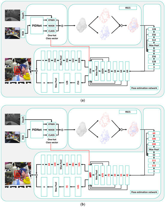
Figure 3.
Comparison of the pipeline before and after pruning of RSCS6D. (a) original network pipeline, (b) optimized network architecture after NS pruning with 50% pruning rate.
NS pruning adaptively reduces channels based on task needs. It decreases model parameters and computation significantly. However, retraining is needed to restore pre-pruning accuracy. By integrating a lightweight pose estimation algorithm based on point cloud keypoints, a compact network can be built. This network has few parameters, low memory usage, and broad applicability.
4. Experiments
In this section, we present the experimental results of our RSCS6D method and compare it with other state-of-the-art approaches.
4.1. Implementation Details
To evaluate the performance of our point cloud keypoint-based pose estimation algorithm, experiments were conducted on the LineMod dataset. The hardware platform used includes a Windows 11 operating system and an NVIDIA GeForce RTX 4090 GPU with 24 GB of VRAM. Our framework was implemented using PyTorch 2.2.2. All experiments were performed on an Intel i9-14900K 3.60 GHz CPU and an NVIDIA GeForce RTX 4090 GPU.
We fine-tuned the PIDNet architecture [28], which was pre-trained on ImageNet [39], to obtain mask images for different categories of target objects. Point cloud keypoints were extracted from RGB-D data using the RSCS method and used for pose estimation. We then trained our improved pose estimation network based on G2L-Net [27]. The network architecture is illustrated in Figure 2.
In the experimental section, we indeed adjusted the network’s hyperparameters to optimize its performance and enhance the precision and efficiency of pose estimation. During this process, we referred to hyperparameter settings from other mature methods in related fields and made targeted adjustments based on the specific needs of our network architecture and task objectives.
For pose prediction, we used mean squared error (MSE) as the loss function, with units in millimeters. The Adam optimizer [40] was employed to train the RSCS6D network. The initial learning rate was set to 0.001 and halved every 50 epochs, with a maximum of 200 epochs. This setup ensures efficient training and convergence of the network.
4.2. Dataset
The LineMod dataset [41] comprises 15,783 images featuring 13 objects, each with approximately 1000 images. Most objects are textureless, and the dataset includes complex scenes with varying lighting conditions, posing significant challenges for pose estimation. Unlike the YCB dataset, which organizes data by scenes, LineMod is organized by objects. Each object’s folder contains depth maps, segmentation masks, RGB images, and text files with pose and annotation information, as well as camera intrinsics and depth scaling factors. LineMod focuses on single-object information; for example, the folder for the first object provides its segmentation masks, pose, and annotations, but not for other objects. Additionally, the dataset provides 3D models of the 13 objects in ply format.
4.3. Evaluation Metrics
In pose estimation tasks, the algorithm outputs a rotation matrix R and translation vector t, which describe the rigid transformation of the target object from the world coordinate system to the camera coordinate system. The accuracy of this transformation can be quantified using the Average Distance (ADD) metric, which measures the average Euclidean distance between the predicted and ground-truth positions of all 3D model points.
Given the ground-truth rotation matrix R and translation vector t, and the predicted rotation matrix Rp and translation vector tp, the ADD is calculated as follows:
Here:
- M is the set of m 3D points of the object in the world coordinate system.
- Rx + t represents the true position of a point in the camera coordinate system.
- Rpx + tp represents the predicted position of the same point.
The ADD metric evaluates the precision of the pose estimation by averaging the Euclidean distances between the predicted and true positions of all model points. This provides a comprehensive measure of how well the estimated pose aligns with the ground truth.
For objects with symmetry, the ADD metric may not accurately reflect the performance of pose estimation algorithms, as symmetry can lead to multiple visually indistinct poses. To address this, DenseFusion introduced the ADD-S metric, which accounts for object symmetry by measuring the average minimum distance between transformed points in the predicted pose and the nearest points on the ground-truth model.
The ADD-S is calculated as follows:
The ADD-S metric addresses the limitations of ADD when evaluating symmetric objects by measuring the average minimum distance from transformed points in the predicted pose to the nearest points on the ground-truth model. Specifically, instead of calculating point-to-point distances, ADD-S computes the average of the minimum distances between each transformed point in the predicted pose and the closest point on the ground-truth model. If this average distance is less than 10% of the object’s diameter, the pose estimation is deemed correct.
4.4. Comparison with the State-of-the-Art Methods
The LineMOD dataset [41] is a widely used benchmark for 6D object pose estimation, featuring 13 objects with significant shape variation. These objects are captured in sequences that include mild occlusions, cluttered backgrounds, textureless surfaces, and varying lighting conditions, making it challenging for accurate pose estimation in real-world scenarios.
Our approach follows the protocol established in previous works [14,20,27,42], which adopts a standard 15%/85% training/test split. This setup ensures a robust evaluation of pose estimation algorithms under diverse and realistic conditions.
Our proposed real-time pose estimation algorithm demonstrates superior performance on the LineMOD dataset, outperforming existing methods such as PVNet [14], PoseCNN [42], DenseFusion [20], and G2L-Net [27]. As shown in Table 1, our algorithm achieves an average ADD accuracy of 99.32% across 13 objects, representing a 0.6% improvement over the best baseline method, G2L-Net (98.7%). Notably, our method sets new records for 11 objects, including ape and bench vise, with perfect ADD-S accuracy of 100% for symmetric objects like eggbox and glue.

Table 1.
Comparison of ADD(-S) metrics for similar algorithms on the LineMOD dataset.
In terms of real-time performance, our algorithm processes at 40 FPS, significantly surpassing DenseFusion (19 FPS) and G2L-Net (28 FPS). Importantly, these results are achieved without the need for refinement post-processing, leveraging the advantages of RGB-D data effectively.
4.5. Comparison of Different Pruning Rates
The lightweight pose estimation algorithm based on NS pruning with different pruning rates shows remarkable advantages on the LineMod dataset, as presented in Table 2. All pruned versions (20–50%) maintain a high accuracy of over 99.3% while keeping the processing speed at 36–37 FPS, surpassing the baseline method. Notably, the 30%-pruned version achieves an average accuracy of 99.5% at 37 FPS with only 10.81 MB of parameters, setting a new benchmark for studies on ten objects including ape and bench vise. Moreover, on symmetric objects eggbox and glue, the ADD-S metric remains at 100%. These results highlight the algorithm’s significant improvements in accuracy, speed, and lightweight performance, with a considerable boost in overall effectiveness compared to traditional methods.
Table 2.
Comparison of lightweight pose estimation with different pruning rates on the LineMOD dataset.
The NS pruning strategy shows excellent model compression ability. Although time increases slightly, the total parameters decrease and the average ADD improves, showing NS pruning’s strong model compression ability. The 30% pruned model offers the best balance, reducing parameters by 17.98% and raising ADD to 99.5% (+0.2%), while running at 37 FPS. The 50% pruned model, with 9.02 MB parameters (a 31.56% reduction), maintains 99.4% ADD, outperforming DenseFusion.
Considering accuracy, speed, and model size, the 30% pruned model is optimal. It achieves 99.5% ADD, an 84.24% parameter reduction to 10.81 MB, and a 39.29% speed boost (37 FPS), making it the final RSCS6D_Pruned algorithm. In summary, combining point cloud keypoint extraction with NS pruning enhances pose estimation in accuracy, speed, and model volume, offering a practical solution for real-time pose estimation in resource-constrained scenarios.
4.6. Visualization Results
In this study, 3D bounding-box visualization assesses various algorithms’ pose estimation performance. The process involves generating a reference bounding box from the target object’s 3D model, computing a predicted-pose bounding box using the algorithm-estimated rotation matrix and translation vector, and projecting it into 2D image space for comparison. On the LineMod dataset (Figure 4, Figure 5 and Figure 6), green, blue, red, and purple boxes denote the ground-truth pose and predictions from G2L-Net, RSCS6D, and RSCS6D_Pruned algorithms. Results show our point-cloud-keypoint-based DL pose estimation algorithm outperforms the G2L-Net baseline. Both the original and quantized versions achieve higher positioning accuracy than the contrast algorithm, with the quantized version performing slightly better.
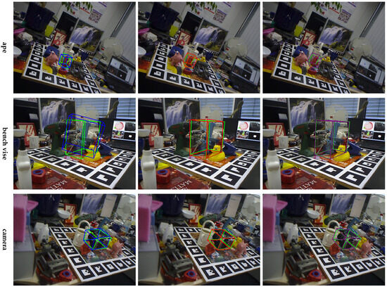
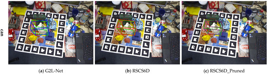
Figure 4.
Visualization of Results I. The green, blue, red, and purple boxes denote the ground truth pose and the predicted poses from the G2L-Net, RSCS6D, and RSCS6D_Pruned algorithms.
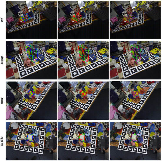
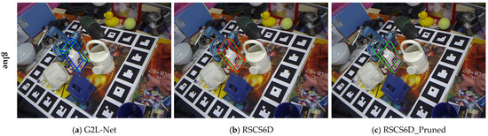
Figure 5.
Visualization of Results II. The green, blue, red, and purple boxes in the figure denote the ground truth pose and the predicted poses from the G2L-Net, RSCS6D, and RSCS6D_Pruned algorithms.
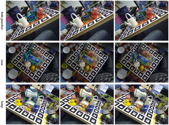
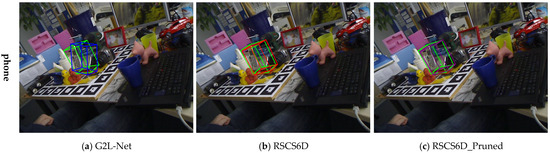
Figure 6.
Visualization of Results III. The green, blue, red, and purple boxes in the figure denote the ground truth pose and the predicted poses from the G2L-Net, RSCS6D, and RSCS6D_Pruned algorithms.
4.7. Limitations
Rigorous experiments validate that our method excels in real-time applications, responding quickly and maintaining high estimation accuracy across various complex scenarios. This demonstrates the potential of our keypoint-based approach to advance 6D pose estimation and to provide new insights and methods for related research and applications.
However, the performance of our algorithm is primarily constrained by the accuracy of the front-end semantic segmentation algorithm. Current depth cameras still have limitations in precision and stability, affecting the performance of the semantic segmentation module and, consequently, the pose estimation accuracy of the entire algorithm. Thus, while our algorithm optimizes pose estimation efficiency and accuracy to some extent, its performance is still limited by the front-end semantic segmentation algorithm and the performance of depth camera hardware.
5. Conclusions
In this paper, we introduce RSCS6D, an innovative real-time 6D object pose estimation framework. By decomposing the complex 6D pose estimation problem into three interconnected sub-tasks—global localization, keypoint extraction, and pose estimation—the framework achieves efficient and accurate pose estimation. During global localization, we employ advanced semantic segmentation to generate mask images, providing precise target area information for subsequent steps. The RSCS algorithm then extracts keypoint clouds from coarse point clouds, reducing data redundancy, accelerating network convergence, and enhancing overall computational efficiency. Finally, our network leverages viewpoint information to accurately predict the rotation and rotation residuals of the keypoint clouds, achieving high-precision pose estimation.
Author Contributions
Conceptualization, W.L. and N.D.; methodology, W.L. and N.D.; software, W.L.; validation, W.L. and N.D.; formal analysis, W.L. and N.D.; investigation, W.L. and N.D.; resources, W.L. and N.D.; data curation, W.L. and N.D.; writing—original draft preparation, W.L.; writing—review and editing, W.L. and N.D.; visualization, W.L. and N.D.; supervision, N.D.; project administration, N.D.; funding acquisition, N.D. All authors have read and agreed to the published version of the manuscript.
Funding
This research was funded by the Department of Science, Technology and Information of the Ministry of Education, grant number 8091B042240.
Institutional Review Board Statement
Not applicable.
Informed Consent Statement
Not applicable.
Data Availability Statement
The original contributions presented in this study are included in the article. Further inquiries can be directed to the corresponding author.
Conflicts of Interest
The authors declare no conflicts of interest.
References
- Yun, W.-H.; Lee, J.; Lee, J.-H.; Kim, J. Object recognition and pose estimation for modular manipulation system: Overview and initial results. In Proceedings of the 2017 14th International Conference on Ubiquitous Robots and Ambient Intelligence (URAI), Jeju, Republic of Korea, 28 June–1 July 2017; pp. 198–201. [Google Scholar]
- Tremblay, J.; To, T.; Sundaralingam, B.; Xiang, Y.; Fox, D.; Birchfield, S. Deep Object Pose Estimation for Semantic Robotic Grasping of Household Objects. arXiv 2018, arXiv:1809.10790. [Google Scholar]
- Chen, X.; Ma, H.; Wan, J.; Li, B.; Xia, T. Multi-view 3D Object Detection Network for Autonomous Driving. In Proceedings of the 2017 IEEE Conference on Computer Vision and Pattern Recognition (CVPR), Honolulu, HI, USA, 21–26 July 2017; pp. 6526–6534. [Google Scholar]
- Geiger, A.; Lenz, P.; Urtasun, R. Are we ready for autonomous driving? The KITTI vision benchmark suite. In Proceedings of the 2012 IEEE Conference on Computer Vision and Pattern Recognition, Providence, RI, USA, 16–21 June 2012; pp. 3354–3361. [Google Scholar]
- Marchand, E.; Uchiyama, H.; Spindler, F. Pose Estimation for Augmented Reality: A Hands-On Survey. IEEE Trans. Vis. Comput. Graph. 2016, 22, 2633–2651. [Google Scholar] [CrossRef] [PubMed]
- Zou, D.; Cao, Q.; Zhuang, Z.; Huang, H.; Gao, R.; Qin, W. An Improved Method for Model-Based Training, Detection and Pose Estimation of Texture-Less 3D Objects in Occlusion Scenes. Procedia CIRP 2019, 83, 541–546. [Google Scholar] [CrossRef]
- Lowe, D.G. Object recognition from local scale-invariant features. In Proceedings of the Seventh IEEE International Conference on Computer Vision, Kerkyra, Greece, 20–27 September 1999; Volume 2, pp. 1150–1157. [Google Scholar]
- Amini, A.; Periyasamy, A.S.; Behnke, S. T6D-Direct: Transformers for Multi-object 6D Pose Direct Regression. In Pattern Recognition; Springer International Publishing: Cham, Switzerland, 2021; pp. 530–544. [Google Scholar]
- Di, Y.; Manhardt, F.; Wang, G.; Ji, X.; Navab, N.; Tombari, F. SO-Pose: Exploiting Self-Occlusion for Direct 6D Pose Estimation. In Proceedings of the 2021 IEEE/CVF International Conference on Computer Vision (ICCV), Montreal, QC, Canada, 10–17 October 2021; pp. 12376–12385. [Google Scholar]
- Hodan, T.; Barath, D.; Matas, J. EPOS: Estimating 6D Pose of Objects With Symmetries. In Proceedings of the IEEE/CVF Conference on Computer Vision and Pattern Recognition (CVPR), Seattle, WA, USA, 13–19 June 2020. [Google Scholar]
- Li, Z.; Wang, G.; Ji, X. CDPN: Coordinates-Based Disentangled Pose Network for Real-Time RGB-Based 6-DoF Object Pose Estimation. In Proceedings of the 2019 IEEE/CVF International Conference on Computer Vision (ICCV), Long Beach, CA, USA, 15–20 June 2019; pp. 7677–7686. [Google Scholar]
- Wang, G.; Manhardt, F.; Tombari, F.; Ji, X. GDR-Net: Geometry-Guided Direct Regression Network for Monocular 6D Object Pose Estimation. In Proceedings of the 2021 IEEE/CVF Conference on Computer Vision and Pattern Recognition (CVPR), Nashville, TN, USA, 20–25 June 2021; pp. 16606–16616. [Google Scholar]
- Amini, A.; Selvam Periyasamy, A.; Behnke, S. YOLOPose: Transformer-Based Multi-object 6D Pose Estimation Using Keypoint Regression. In Intelligent Autonomous Systems 17; Springer Nature: Cham, Switzerland, 2023; pp. 392–406. [Google Scholar]
- Peng, S.; Zhou, X.; Liu, Y.; Lin, H.; Huang, Q.; Bao, H. PVNet: Pixel-Wise Voting Network for 6DoF Object Pose Estimation. IEEE Trans. Pattern Anal. Mach. Intell. 2022, 44, 3212–3223. [Google Scholar] [CrossRef] [PubMed]
- He, Y.; Sun, W.; Huang, H.; Liu, J.; Fan, H.; Sun, J. PVN3D: A Deep Point-Wise 3D Keypoints Voting Network for 6DoF Pose Estimation. In Proceedings of the 2020 IEEE/CVF Conference on Computer Vision and Pattern Recognition (CVPR), Seattle, WA, USA, 13–19 June 2020; pp. 11629–11638. [Google Scholar]
- He, Y.; Huang, H.; Fan, H.; Chen, Q.; Sun, J. FFB6D: A Full Flow Bidirectional Fusion Network for 6D Pose Estimation. In Proceedings of the 2021 IEEE/CVF Conference on Computer Vision and Pattern Recognition (CVPR), Nashville, TN, USA, 20–25 June 2021; pp. 3002–3012. [Google Scholar]
- Wu, Y.; Zand, M.; Etemad, A.; Greenspan, M. Vote from the Center: 6 DoF Pose Estimation in RGB-D Images by Radial Keypoint Voting. In Computer Vision—ECCV 2022; Springer Nature: Cham Switzerland, 2022; pp. 335–352. [Google Scholar]
- Zhou, J.; Chen, K.; Xu, L.; Dou, Q.; Qin, J. Deep Fusion Transformer Network with Weighted Vector-Wise Keypoints Voting for Robust 6D Object Pose Estimation. In Proceedings of the 2023 IEEE/CVF International Conference on Computer Vision (ICCV), Paris, France, 1–6 October 2023; pp. 13921–13931. [Google Scholar]
- Su, Y.; Saleh, M.; Fetzer, T.; Rambach, J.; Navab, N.; Busam, B.; Stricker, D.; Tombari, F. ZebraPose: Coarse to Fine Surface Encoding for 6DoF Object Pose Estimation. In Proceedings of the 2022 IEEE/CVF Conference on Computer Vision and Pattern Recognition (CVPR), New Orleans, LA, USA, 18–24 June 2022; pp. 6728–6738. [Google Scholar]
- Wang, C.; Xu, D.; Zhu, Y.; Martín-Martín, R.; Lu, C.; Fei-Fei, L.; Savarese, S. DenseFusion: 6D Object Pose Estimation by Iterative Dense Fusion. In Proceedings of the 2019 IEEE/CVF Conference on Computer Vision and Pattern Recognition (CVPR), Long Beach, CA, USA, 15–20 June 2019; pp. 3338–3347. [Google Scholar]
- Mo, N.; Gan, W.; Yokoya, N.; Chen, S. ES6D: A Computation Efficient and Symmetry-Aware 6D Pose Regression Framework. In Proceedings of the 2022 IEEE/CVF Conference on Computer Vision and Pattern Recognition (CVPR), New Orleans, LA, USA, 18–24 June 2022; pp. 6718–6727. [Google Scholar]
- Jiang, X.; Li, D.; Chen, H.; Zheng, Y.; Zhao, R.; Wu, L. Uni6D: A Unified CNN Framework without Projection Breakdown for 6D Pose Estimation. In Proceedings of the 2022 IEEE/CVF Conference on Computer Vision and Pattern Recognition (CVPR), New Orleans, LA, USA, 18–24 June 2022; pp. 11164–11174. [Google Scholar]
- Sun, M.; Zheng, Y.; Bao, T.; Chen, J.; Jin, G.; Wu, L.; Zhao, R.; Jiang, X. Uni6Dv2: Noise Elimination for 6D Pose Estimation. In Proceedings of the International Conference on Artificial Intelligence and Statistics, Virtual, 28–30 March 2022. [Google Scholar]
- Chen, S.; Li, X.; Wang, Z.; Prisacariu, V.A. DFNet: Enhance Absolute Pose Regression with Direct Feature Matching. In Computer Vision—ECCV 2022; Springer Nature: Cham, Switzerland, 2022; pp. 1–17. [Google Scholar]
- Shavit, Y.; Ferens, R.; Keller, Y. Coarse-to-Fine Multi-Scene Pose Regression With Transformers. IEEE Trans. Pattern Anal. Mach. Intell. 2023, 45, 14222–14233. [Google Scholar] [CrossRef] [PubMed]
- Sattler, T.; Zhou, Q.; Pollefeys, M.; Leal-Taixe, L. Understanding the Limitations of CNN-Based Absolute Camera Pose Regression. In Proceedings of the IEEE/CVF Conference on Computer Vision and Pattern Recognition (CVPR), Seattle, WA, USA, 13–19 June 2019. [Google Scholar]
- Chen, W.; Jia, X.; Chang, H.J.; Duan, J.; Leonardis, A. G2L-Net: Global to Local Network for Real-Time 6D Pose Estimation With Embedding Vector Features. In Proceedings of the 2020 IEEE/CVF Conference on Computer Vision and Pattern Recognition (CVPR), Seattle, WA, USA, 13–19 June 2020. [Google Scholar]
- Xu, J.; Xiong, Z.; Bhattacharyya, S.P. PIDNet: A Real-Time Semantic Segmentation Network Inspired by PID Controllers. In Proceedings of the 2023 IEEE/CVF Conference on Computer Vision and Pattern Recognition (CVPR), Vancouver, BC, Canada, 17–24 June 2023; pp. 19529–19539. [Google Scholar]
- Liu, Z.; Li, J.; Shen, Z.; Huang, G.; Yan, S.; Zhang, C. Learning Efficient Convolutional Networks Through Network Slimming. In Proceedings of the IEEE International Conference on Computer Vision (ICCV), Venice, Italy, 22–29 October 2017. [Google Scholar]
- Zhong, Y. Intrinsic shape signatures: A shape descriptor for 3D object recognition. In Proceedings of the 2009 IEEE 12th International Conference on Computer Vision Workshops, ICCV Workshops, Kyoto, Japan, 27 September–4 October 2009; pp. 689–696. [Google Scholar]
- Sipiran, I.; Bustos, B. Harris 3D: A robust extension of the Harris operator for interest point detection on 3D meshes. Vis. Comput. 2011, 27, 963–976. [Google Scholar] [CrossRef]
- Hänsch, R.; Weber, T.; Hellwich, O. Comparison of 3D interest point detectors and descriptors for point cloud fusion. ISPRS Ann. Photogramm. Remote Sens. Spat. Inf. Sci. 2014, II-3, 57–64. [Google Scholar] [CrossRef]
- Wang, X.; Chen, H.; Wu, L. Feature extraction of point clouds based on region clustering segmentation. Multimed. Tools Appl. 2020, 79, 11861–11889. [Google Scholar] [CrossRef]
- Chen, H.; Sun, D.; Liu, W.; Wu, H.; Liang, M.; Liu, P.X. A Novel Approach to the Extraction of Key Points From 3-D Rigid Point Cloud Using 2-D Images Transformation. IEEE Trans. Geosci. Remote Sens. 2022, 60, 5703815. [Google Scholar] [CrossRef]
- Arun, K.S.; Huang, T.S.; Blostein, S.D. Least-Squares Fitting of Two 3-D Point Sets. IEEE Trans. Pattern Anal. Mach. Intell. 1987, PAMI-9, 698–700. [Google Scholar] [CrossRef] [PubMed]
- Fischler, M.A.; Bolles, R.C. Random Sample Consensus: A Paradigm for Model Fitting with Applications to Image Analysis and Automated Cartography. In Readings in Computer Vision; Morgan Kaufmann: San Francisco, CA, USA, 1987; pp. 726–740. [Google Scholar]
- Comaniciu, D.; Meer, P. Mean shift: A robust approach toward feature space analysis. IEEE Trans. Pattern Anal. Mach. Intell. 2002, 24, 603–619. [Google Scholar] [CrossRef]
- Yang, L.; Li, Y.; Li, X.; Meng, Z.; Luo, H. Efficient plane extraction using normal estimation and RANSAC from 3D point cloud. Comput. Stand. Interfaces 2022, 82, 103608. [Google Scholar] [CrossRef]
- Deng, J.; Dong, W.; Socher, R.; Li, L.J.; Li, K.; Fei-Fei, L. ImageNet: A large-scale hierarchical image database. In Proceedings of the 2009 IEEE Conference on Computer Vision and Pattern Recognition, Miami, FL, USA, 20–25 June 2009; pp. 248–255. [Google Scholar]
- Kingma, D.P.; Ba, J. Adam: A Method for Stochastic Optimization. In Proceedings of the 3rd International Conference on Learning Representations, ICLR 2015, San Diego, CA, USA, 7–9 May 2015. [Google Scholar]
- Hinterstoisser, S.; Holzer, S.; Cagniart, C.; Ilic, S.; Konolige, K.; Navab, N.; Lepetit, V. Multimodal templates for real-time detection of texture-less objects in heavily cluttered scenes. In Proceedings of the 2011 International Conference on Computer Vision, Barcelona, Spain, 6–13 November 2011; pp. 858–865. [Google Scholar]
- Xiang, Y.; Schmidt, T.; Narayanan, V.; Fox, D. PoseCNN: A Convolutional Neural Network for 6D Object Pose Estimation in Cluttered Scenes. In Proceedings of the Robotics: Science and Systems, Pittsburgh, PA, USA, 26–30 June 2018. [Google Scholar]
Disclaimer/Publisher’s Note: The statements, opinions and data contained in all publications are solely those of the individual author(s) and contributor(s) and not of MDPI and/or the editor(s). MDPI and/or the editor(s) disclaim responsibility for any injury to people or property resulting from any ideas, methods, instructions or products referred to in the content. |
© 2025 by the authors. Licensee MDPI, Basel, Switzerland. This article is an open access article distributed under the terms and conditions of the Creative Commons Attribution (CC BY) license (https://creativecommons.org/licenses/by/4.0/).