1. Introduction
Prognostics and Health Management (PHM) focuses on condition monitoring and the extrapolation of degradation trends based on recent observations [
1,
2,
3]. Among the established techniques for monitoring the state of machinery, oil analysis is the most popular. Oil monitoring is mainly concerned with the analysis of sampled oil to detect wear-related problems [
4,
5,
6,
7]. Shell in its advisory report indicates that oil contamination causes approximately 70% of in-service failures in diesel engines, of which 50% are the result of wear-related problems [
8]. The wear is complex, including multiple friction pairs, such as wet clutches, transmission gears, sealing rings, bearings, and confluence planetary gear trains.
The wear describes the degradation of mechanical systems to some degree. However, unless the wear is directly observable, such as in the case of a brake pad, it is difficult to quantify it in general. For most mechanical systems, wear is not directly observable and can only be assessed via other measured condition information data such as the concentrations of metal elements. The concentration of metal within oil samples is a good indicator of wear and has been widely used for wear evaluation [
8,
9,
10,
11,
12]. Wang [
8] used metal concentrations to describe the deterioration of a maintained plant. Vališ et al. [
9] considered the metal concentration as a potential failure indicator and then proposed a linear regression model to determine a linear course of metal particle generation. Zheng et al. [
10] used the Wiener process to model metal concentrations and thus optimized the planned maintenance interval of the power shift steering transmission.
However, in practical scenarios, many factors such as oil top-ups, wear particle removal, and different measurement methods can disturb the observation of the metal concentration, thereby causing the observed data to deviate from the actual physical degradation. This distortion (deviation) indicates that it is infeasible to directly use the observed data to evaluate the wear condition. In other words, it is necessary to recover the actual physical degradation curve based on the observed data.
Macián et al. [
13] considered the influence of oil consumption and replenishment and developed an analytical approach to the wear rate of internal combustion engines based on spectrometric oil analysis. Bagshaw et al. [
14] used oil volume correction to transform the observed data into absolute wear values. Feng et al. [
15] considered the effect of the time-varying wear coefficient. A model of wear debris concentration was built based on Kragelsky’s method with different wear coefficients in corresponding wear stages. However, the literature mentioned above assumes that the refilling is carried out at predetermined maintenance intervals [
13,
14,
15,
16] and does not consider dynamic, non-periodic oil top-ups driven by real-time operational conditions. Moreover, the above models were established based on particular mechanical structures such as an internal combustion engine, a continuous flow stirred tank reactor (CFSTR), or a gearbox, thereby restricting their applications.
Considering the disturbance caused by non-periodic oil top-ups, a piecewise linear method was employed to address the resulting variations in oil spectrum analysis [
17,
18]. The Hermite interpolation approach was used to model the wear characteristics [
19]. The grey model and AR time series model were also adopted [
20]. However, these methods rely on subjective judgments to identify oil top-up points and use local observed information to correct the data. This indicates that these methods not only lack objectivity but also do not make full use of existing observation information.
This paper focuses on rectifying observed degradation data distorted by non-periodic oil top-ups. As shown in
Figure 1 (Vehicle 1 dataset), the observed data exclusively contain Cu (copper) concentration measurements with the corresponding sampling time but lack documentation of oil top-up times and quantities. Detailed experimental information is provided in
Section 4. It is evident that the acquired Cu concentration exhibits non-monotonic behavior despite the inherent monotonicity of mechanical wear processes. This discrepancy stems from dilution effects caused by fresh oil additions. The contributions of this paper can be summarized as follows:
A statistical correction model is proposed to process degradation data that are disturbed by non-periodic oil top-ups. The proposed model can not only automatically identify the locations of oil top-up points but also globally correct the observed degradation data.
A three-step explosion search algorithm is developed, enabling robust parameter estimation through both parametric and non-parametric approaches.
The corrected degradation data can reflect the actual physical degradation; thus, these corrected data can be used to assess system conditions and predict a failure.
Notably, while the methodology is developed through wear degradation analysis, its data-driven architecture ensures generalizability to various degradation monitoring scenarios requiring measurement distortion correction.
The rest of the paper is organized as follows: The proposed methodology is presented in detail in
Section 2. In
Section 3, we perform some numerical simulations. Case studies are shown in
Section 4.
Section 5 provides discussion and conclusions.
2. Methodology
2.1. Data and Model
The actual physical degradation serves as a “health indicator” for system wear; however, the observation of the physical degradation process is affected by oil top-ups. To be specific, once the fresh oil is added, the observed degradation data, such as the concentration of metal elements, will be diluted. Therefore, it is necessary to correct the observed degradation data. Before establishing the model, we have the following assumptions: If the mass of the oil added is unknown, then the observed degradation data, namely, the concentrations of metal elements, are diluted in the same ratio each time fresh oil is added. This indicates that the oil top-up effect can be described by a constant.
The definitions of all variables and mathematical symbols are listed in
Table 1. If the observed error cannot be neglected, then the observed degradation is random, namely,
where
is the random error and follows a normal distribution with zero mean and standard deviation
.
We established a model to describe the relationship between observed degradation data without measurement errors and the actual physical degradation process. Typically, we consider three cases: complete observation data, partially missing data, and completely missing data.
Case I: The observed data consist of
, representing complete observations. If fresh oil is added after the
th observation, then the concentration becomes
; otherwise, it remains
. Therefore, neglecting measurement errors, the observed degradation
consists of two components: the cumulative degradation
and the increment in the degradation process
. Formally, the correction model can be expressed as follows:
Case II: The observed data consist of
, which are partial missing observations. Since the effects of oil top-ups are unknown, their mean value
is adopted. Therefore, in this case, the model can be represented as follows:
Case III: The observed data consist of
, which are complete missing observations. The formula of the model is also given by Equation (
3). However, we note that
is unknown in this case.
2.2. Parameter Estimation
Indeed, engineers primarily focus on the actual degradation data . Case II can be considered a bridge, and it links Case I and Case III. Thus, we start with Case II to explore the parameter estimation approaches.
2.2.1. Parametric Estimation Approach
If the parametric representation of the physical degradation process can be derived based on available physical theories, then the parametric estimation approach is a good choice. Here, the physical degradation h is a function of the observed time t and the unknown parameter vector , given by .
Through a simple derivation, Equation (
3) for
Case II can be reformulated as follows:
where
and
. Under the assumption that the observed error follows the normal distribution, the likelihood function is given by
We use traditional optimization methods such as the Gauss–Newton iteration method to maximize this likelihood function. Then, the maximum likelihood estimations of the unknown parameters obtained are denoted by .
Similarly, we can obtain the maximum likelihood estimations for Case I. Compared with Case I, there is an additional parameter under Case II.
Under Case III, the locations of oil top-up points are unknown; therefore, it is necessary to identify them. Inspired by the monotonic non-decreasing nature of the physical degradation, we propose an explosion search algorithm, which detects the oil top-up points from the decreased points. Note that the decreased point refers to the point where the observed degradation is lower than the previous point.
More specifically, the indicator of whether the fresh oil is added may be 1 or 0 at the decreased point, while it is fixed to 0 at the increased point. Therefore, with
d decreased points, there are
candidate degradation paths. For each candidate degradation path, we calculate its maximum likelihood estimation based on Equation (
4). Then, we obtain
estimations and select one with the minimum residual sum of squares as the final estimation. The procedure for the parametric estimation approach for
Case III is described by Algorithm 1 in detail.
| Algorithm 1: The three-step explosion search algorithm |
Step 1: Find the candidate oil top-up paths: Find the locations of the decreased points; Calculate the number of the decreased points, denoted by d; Define the candidate oil top-up paths . Step 2: Calculate the maximum likelihood estimation of each candidate oil top-up path: for all do Calculate maximum likelihood estimations ( , by Equation ( 4), where ; Calculate the residual sum of squares, . end for Step 3: Obtain the final estimation:
|
In addition to point estimation, engineers may be also interested in interval estimation. We take Case II as an example to illustrate how to use the percentile bootstrap to construct confidence intervals.
- (1)
Generate bootstrap sample , , where , , and are independent and identically distributed residuals generated from .
- (2)
Calculate the maximum likelihood estimation of the bth bootstrap sample , .
- (3)
The
percentile bootstrap interval of
is given by
where
and
are the lower and upper
quantiles of
, respectively.
2.2.2. Non-Parametric Estimation Approach
To avoid possible model misspecification in a parametric analysis, we consider an alternative approach, namely, the non-parametric estimation approach.
Under
Case II, we use a natural cubic smoothing spline [
21] to fit the actual physical degradation curve. The natural cubic smoothing spline is a smooth and continuous twice differentiable curve that minimizes the penalized sum of squares. The penalized sum of squares consists of two parts: the residual sum of squares that quantifies the goodness-of-fit to the data, and the roughness penalty term based on the second derivative. More specifically, we have the following optimization problem:
where
,
is a positive smoothing parameter, controlling the trade-off between fidelity to the data and the roughness of the function estimation, and the constraint condition
, to some extent, ensures that the estimation of the actual physical degradation curve is monotonically non-decreasing. Then, the interior-point method is used to solve this problem (see
Appendix A for more details).
Under
Case III, due to the absence of
, the three-step explosion search algorithm in the previous subsection is used in the non-parametric estimation approach. Note that its second step is replaced by the non-parametric estimation based on Equation (
5). Moreover, similarly to the parametric estimation approach, we can compute the bootstrap confidence interval for non-parametric estimation.
2.3. Failure Prediction
The estimation of the actual physical degradation curve, which is also a correction to the observed degradation, can reflect the actual physical degradation well. Consequently, this estimation can be used to assess the system state and predict a failure. A failure occurs when the degradation curve
hits the failure threshold
that is empirically predetermined by engineers. According to the concept of First Hitting Time (FHT), the lifetime
T of the system is defined as
Moreover, the Remaining Useful Life (RUL) is predicted; that is,
.
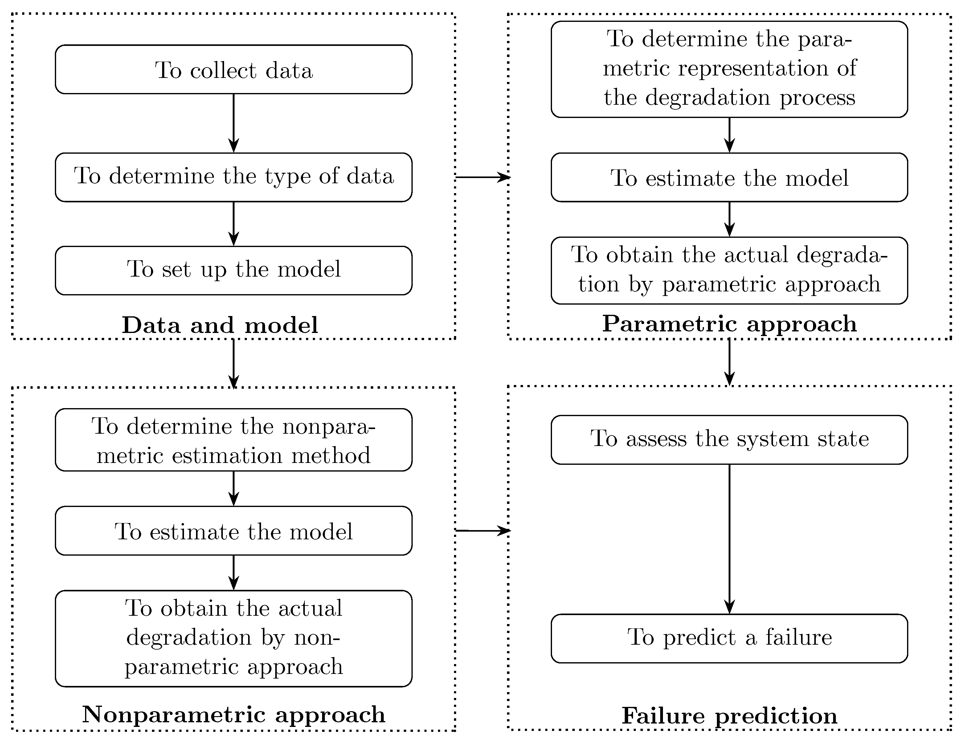
2.4. Implementation Procedure
In order to illustrate how to use our methodology, we show its implementation procedure in
Figure 2.
3. Numerical Simulations
In order to compare the proposed methodology with the piecewise linear method [
17], two kinds of degradation functions are considered in this subsection.
Specifically, the observed degradations is given by , where . Here, the actual degradation equals . The observed points with are equally spaced in . The measure error follows a normal distribution with zero mean and standard deviation . follows Bernoulli distribution with the parameter . follows the normal distribution with mean and variance , and we set . We simulate 1000 datasets based on the above parameter configuration and calculate the estimations for each dataset.
Since it is impossible to enumerate all degradation patterns, here, we will only choose certain representative patterns for illustration. We consider the following two degradation scenarios for all the three cases defined in
Section 2:
Scenario (I): The actual degradation is linear given by where .
Scenario (II): The actual degradation is non-linear given by where .
For the parameter estimations obtained by the parametric approach, we calculate the mean of these 1000 estimations, as well as the standard deviation (SD) and the mean square error (MSE). The results of
Scenario (I) and those of
Scenario (II) are shown in
Table 2 and
Table 3, respectively. We can see that the SD and MSE are very small for each parameter. Moreover, the mean values of estimations are very close to the true values. These results show that the proposed parametric approach indeed works well.
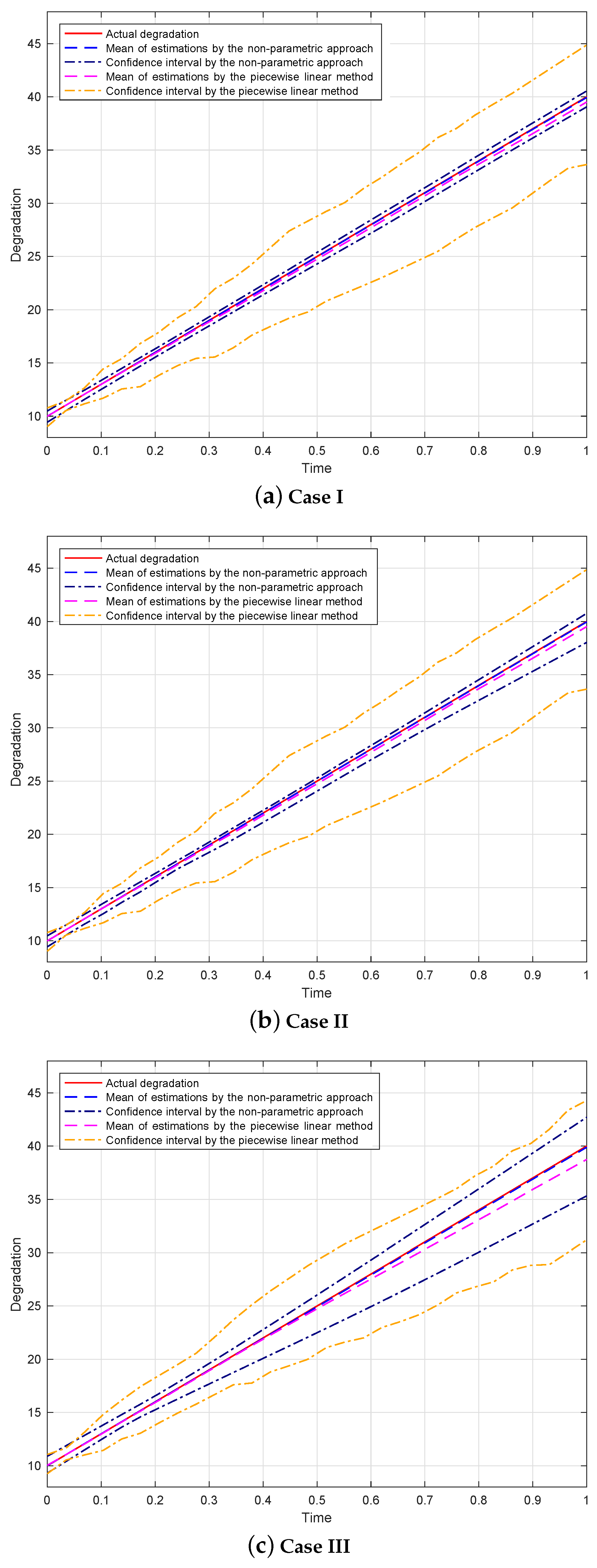
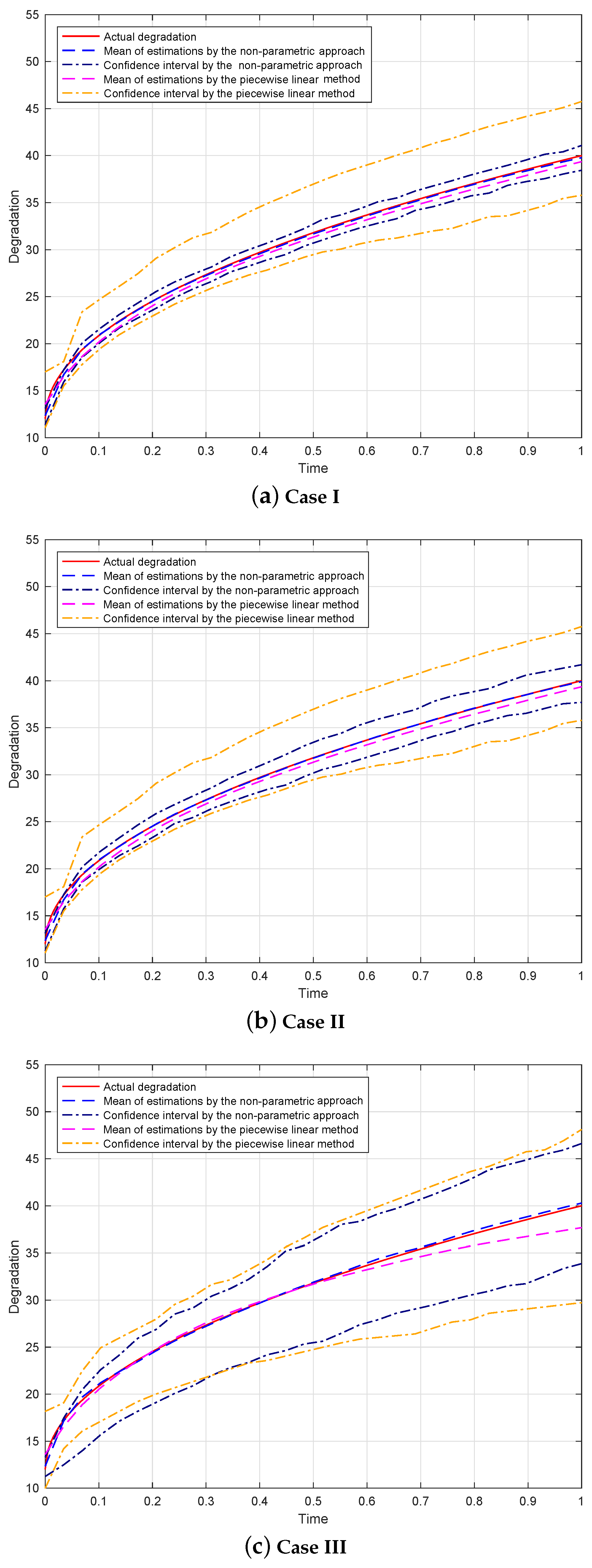
The results obtained by the non-parametric approach in
Scenario (I) and
Scenario (II) are, respectively, plotted in
Figure 3 and
Figure 4. The top, middle, and bottom rows display the non-parametric estimations for
Case I,
Case II, and
Case III, respectively. The 95% point-wise confidence intervals are computed by taking the
th percentile and the
th percentile of 1000 estimations at each observed time point. It can be seen that the mean values of the non-parametric estimations are very close to the actual degradation curve and the confidence intervals are narrow. These results indicate that the proposed non-parametric approach performs well.
Moreover, the piecewise linear method [
17] is also used in our simulation. The results obtained by the piecewise linear method are also shown in
Figure 3 and
Figure 4. We can see that the following is true: (a) The mean values of estimations obtained by the piecewise linear method are farther away from the actual degradation curve than those obtained by our non-parametric approach. (b) The confident intervals obtained by the piecewise linear method are wider than those obtained by our non-parametric approach. These results imply that the performances of our non-parametric approach are better than those of the piecewise linear method.
In addition, from
Table 2 and
Table 3 and
Figure 3 and
Figure 4, we can conclude that the estimations for
Case I are more precise than those for
Case II, and the estimates for
Case II are better than those for
Case III. This is reasonable, because the more complete the observed data, the more accurate the obtained estimations. Moreover, we computed the coverage probabilities for the
bootstrap confidence intervals, and we list them in
Table 4 and
Table 5. We can observe that the coverage probabilities are all around 95%. This indicates that our model and the corresponding estimation approaches are effective.
Overall, simulation studies show that our model and the corresponding estimation approaches perform well whether the degradation is linear or non-linear. Moreover, our methodology can recover the actual degradation curve better than the piecewise linear method; therefore, we can conclude that our methodology is superior to the piecewise linear method.
4. Case Studies
In this section, we validate the practical applicability of our proposed degradation model by investigating wear degradation data in the power-shift steering transmission (PSST) of tracked vehicles. PSST is characterized by its high loading capacity. The wear in PSST is complex, occurring by the plastic displacement of surface and near-surface material and by the detachment of particles. The metal particles of various shapes and sizes that are formed by the wear are distributed in the oil as contaminants.
Our experiment is an on-road test rather than a laboratory test. To be specific, the tracked vehicle runs on the road and the oil is sampled at discrete time points. Then, the spectrometric oil analysis technique is used to measure concentrations of metal particles within oil samples. In consideration of oil consumption, at some sampling points, fresh oil is added to the PSST after sampling. The Cu (copper) element represents the overall wear level. Therefore, the observations for Cu in the PSST of Vehicle 1 are shown in
Figure 1 and listed in
Table 6. We can see that the concentrations of Cu are non-monotone although the actual wear process is monotone. This is due to the fact that the addition of fresh oil reduces the concentration of Cu in the PSST.
Consequently, it is necessary to correct the observed data and thus recover the actual degradation curve. Unfortunately, as shown in
Table 6, the data obtained only include the sampling time and the observed concentration, without the oil top-up time and the oil top-up quantity. Thus, we model these observed data based on
Case III defined in
Section 2 and then, respectively, use the parametric and non-parametric approaches to estimate the parameters of the model.
In the parametric approach, the parametric representation of the physical degradation process is critical. The fresh oil is added after running for some time; therefore, the first few observed concentrations are not affected by the fresh oil and can represent the actual physical degradation. According to the first few observed concentrations in
Figure 1, we can assume that the running time and actual physical degradation are non-linearly expressed as follows:
where
t is the time and
are unknown parameters.
In the non-parametric approach, as introduced in
Section 2, we use a natural cubic smoothing spline to fit the actual physical degradation curve.
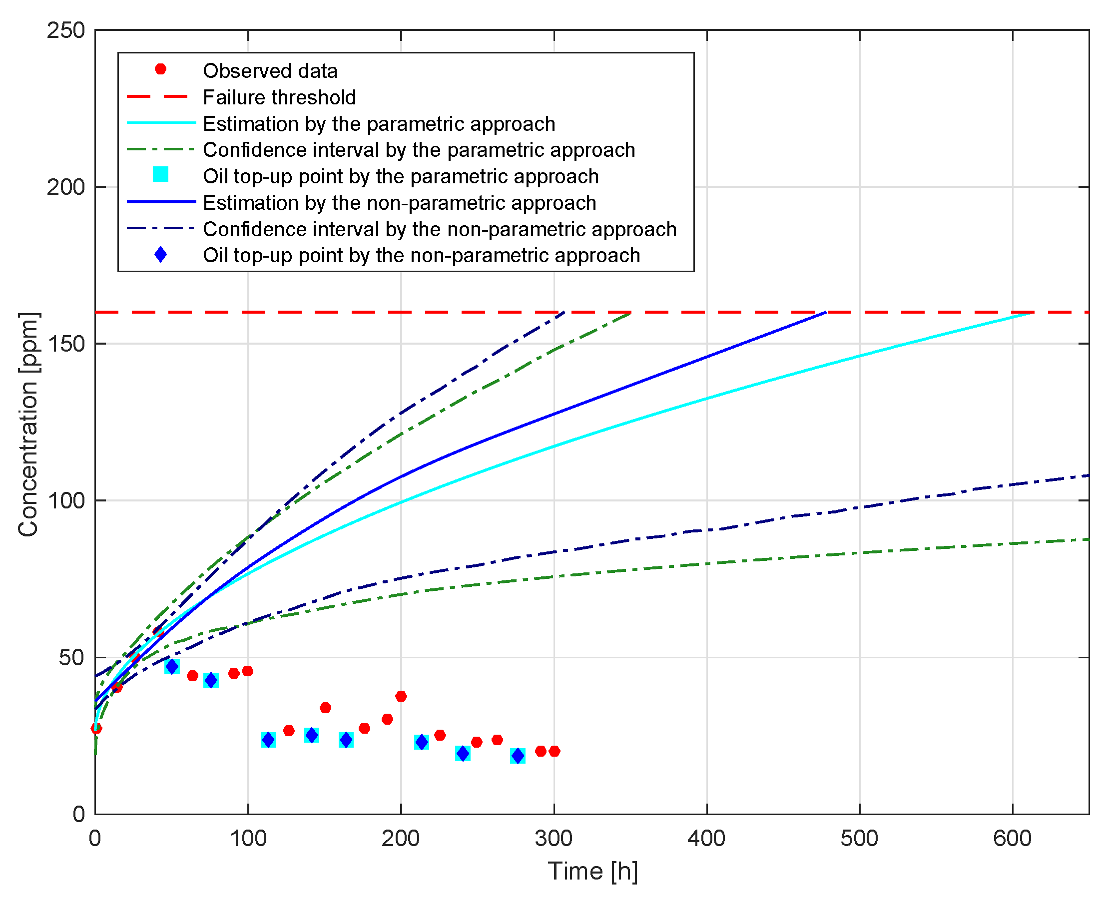
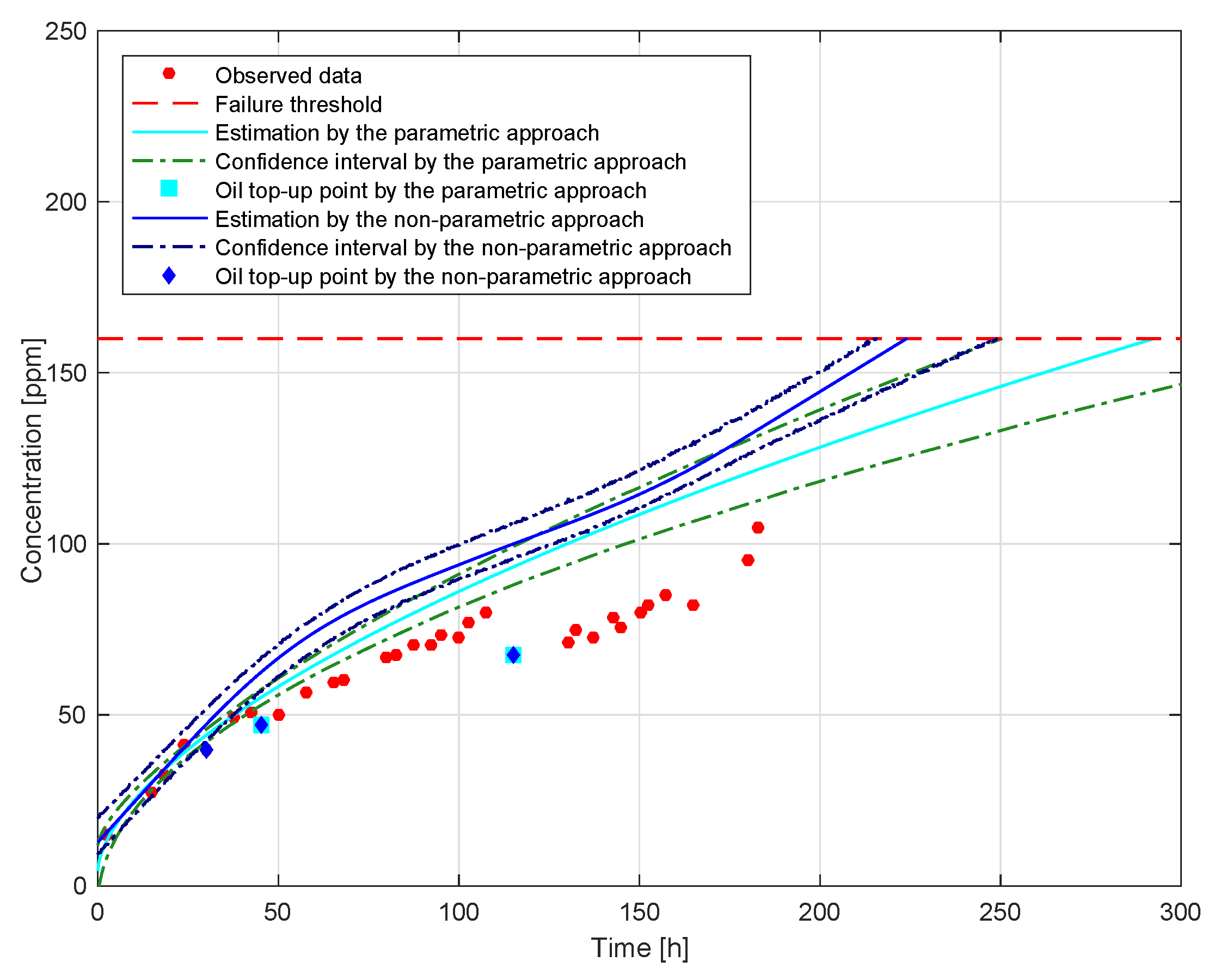
Figure 5 shows the results for the parametric and non-parametric approaches, including the observed data, the detected oil top-up points, the actual degradation (the corrected curve), and the bootstrap confidence intervals. We can see that the number of oil top-ups is relatively large. Frequent oil top-ups may be due to high-intensity work or a high leakage rate. Moreover, we notice that there is a big gap between the observed degradation and the corrected one. The “uncorrected” (observed) data are non-monotone and relative while the “corrected” (actual) data are monotone and absolute. This implies that the corrected curve reflects the actual physical degradation process better than the observed data. Therefore, it is meaningful to use our methodology to correct the observed data.
Based on actual experience, the failure threshold of Cu is set to 160 ppm.
Figure 5 also shows the FHT for failure occurrence based on parametric and non-parametric approaches. Furthermore, we can see that the actual wear degradation has not reached the failure threshold yet, and thus Vehicle 1 can still work normally for a while.
The observed degradation data in the PSST of Vehicle 2 are shown in
Table 7.
Figure 6 shows the results obtained, respectively, by the parametric approach and the non-parametric approach. It can be seen that the number of oil top-ups is relatively small, and there is a small gap between the observed degradation and the corrected one.
According to the above two examples, our methodology can correct the distortion data and obtain an estimation of the actual degradation curve. The “uncorrected” (observed) concentration only indicates that wear is taking place while the “corrected” (actual) concentration reflects the degree of wear. Therefore, our methodology can avoid the misdiagnosis of wear condition to some degree.
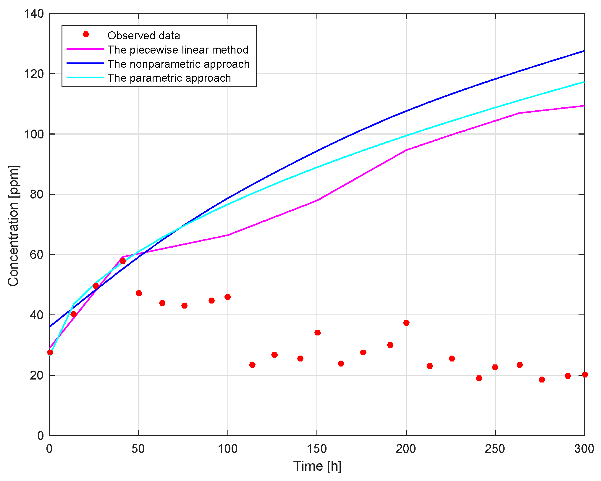
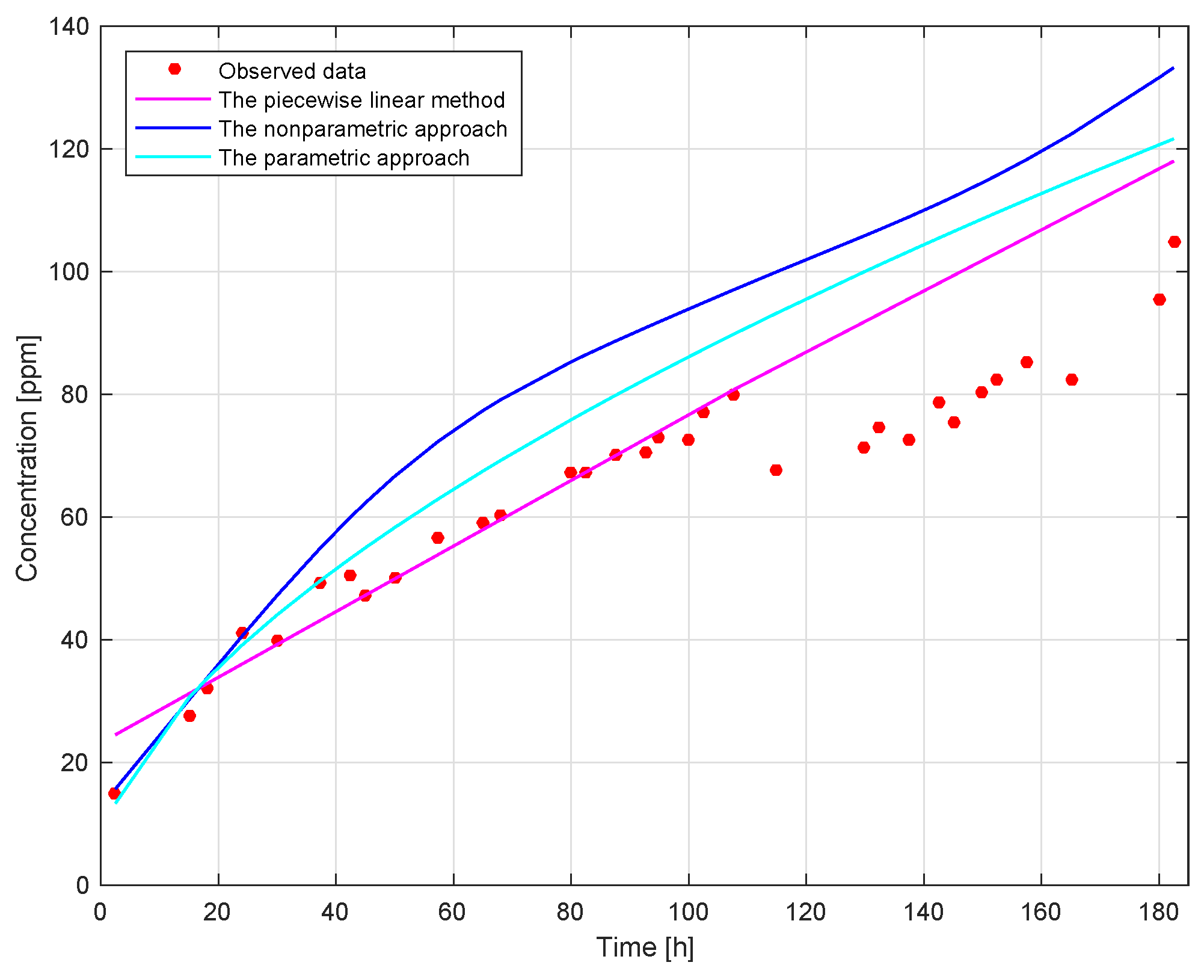
Furthermore, we compared our methodology with the piecewise linear method [
17]. The results shown in
Figure 7 and
Figure 8 can be summarized as follows:
The estimation of the actual degradation obtained by the piecewise linear method is the minimum among the three methods. This indicates that the possibility of missing alarm is relatively high and the possibility of false alarm is relatively low if the piecewise linear method is used. Therefore, if engineers’ goal is to minimize the possibility of false alarms, then the piecewise linear method is a good choice.
The estimation of the actual degradation obtained by the non-parametric approach is the maximum among the three methods. This means that the possibility of missing an alarm is relatively low and the possibility of a false alarm is relatively high if the non-parametric approach is used. Consequently, when engineers want to pay more attention on the possibility of missing an alarm, the non-parametric approach should be used.
The estimation of the actual degradation obtained by the parametric approach is located in the middle of the three methods. Therefore, if engineers are very certain about the parametric representation of the physical degradation process, it is recommended to use the parametric approach.
It should be noted that the piecewise linear method has three drawbacks: Firstly, it uses local observations to piecewisely correct the observed degradation, rather than global observations. Secondly, it uses engineers’ subjective determination to identify the disturbed points, thereby lacking objectivity. Thirdly, it assumes that the actual degradation curve is linear. However, the actual degradation is non-linear in many scenarios.
In conclusion, compared with the piecewise linear method, our model and the corresponding estimate approaches have some obvious advantages, as follows:
Our model is established based on the global observed data, so it can locate more valuable information in the observed data.
Our model can identify the disturbed points automatically, thereby avoiding subjective judgment and improving the objectivity and accuracy.
Both the parametric approach and the non-parametric approach can describe various kinds of degradation patterns, whether linear or non-linear. Therefore, our approaches have wider applicability and practicability.
5. Discussion and Conclusions
As we all know, most of the actual degradation process is monotone. However, in some circumstances, such as the observation being disturbed by some factors, the observed degradation data lose their monotonicity and are distorted. In this paper, we propose a model to characterize this distorted case and come up with the corresponding approach to solving this model.
Compared with the piecewise linear method [
17], the simulation results demonstrate that our methodology can automatically identify disturbed points, thereby avoiding the subjective judgment required for the piecewise linear method, and can also more accurately recover the actual degradation curves. Importantly, our method is flexible enough to model both linear and non-linear degradation patterns, which expands its applicability and practical utility beyond that of the piecewise linear method. Case studies demonstrate that our methodology can describe the effect of disturbed factors, as well as recovering the actual degradation curve and automatically identifying the disturbed points. This is significantly meaningful for condition monitoring, because it avoids a false diagnosis of degradation to some degree.
We remark that our proposed model can be generalized to a situation where the physical degradation process is monotone while the observed process is not monotone due to the disturbance of a point process. Specifically, without observed error, the observation is a perturbation of the actual physical degradation process, as follows:
where the actual physical degradation
is a monotone process, such as a Gamma process or inverse Gaussian process,
is a marked point process, the random variable
indicates the influence of disturbance, and the random variable
takes one of two values, 0 or 1; it equals 1 when there is an existing disturbance at the
ith observed time
and equals 0 otherwise. If the observed error cannot be neglected, then the observed degradation is as follows:
where
is the stochastic observed error with
.
Particle morphology influences wear mechanism identification. Therefore, these morphological parameters should be incorporated into future investigations. Furthermore, while the current validation is limited to the PSST, extending model verification to multiple machinery types would strengthen the generalizability. Additionally, integrating data-driven methodology with equipment-specific engineering knowledge represents a critical direction for subsequent research.


