Article

A Study on Denoising Autoencoder Noise Selection for Improving the Fault Diagnosis Rate of Vibration Time Series Data

1
ADIALAB, 702-1, 57 Centum-dong-ro, Haeundae-gu, Busan 48059, Republic of Korea
2
Department of Naval Architecture and Ocean Engineering, College of Ocean Sciences, Gyeongsang National University, 11-dong, 2 Tongyeonghaean-ro, Tongyeong-si 53064, Republic of Korea
*
Author to whom correspondence should be addressed.
Appl. Sci. 2025, 15(12), 6523; https://doi.org/10.3390/app15126523
Submission received: 18 April 2025 / Revised: 29 May 2025 / Accepted: 2 June 2025 / Published: 10 June 2025
(This article belongs to the Section Mechanical Engineering)

Abstract

This study analyzes the impact of different types of random noise applied in Denoising Autoencoder (DAE) training on fault diagnosis performance, with the aim of improving noise removal for vibration time series data. While conventional studies typically train DAEs using Gaussian random noise, such noise does not fully reflect the complex noise patterns observed in real-world industrial environments. Therefore, this study proposes a novel approach that uses high-frequency noise components extracted from actual vibration data as training noise for the DAE. Both Gaussian and high-frequency noise were used to train separate DAE models, and statistical features (mean, RMS, standard deviation, kurtosis, skewness) were extracted from the denoised signals. The fault diagnosis rates were calculated using One-Class Support Vector Machines (OC-SVM) for performance comparison. As a result, the model trained with high-frequency noise achieved a 0.0293 higher average F1-score than the Gaussian-based model. Notably, the fault detection accuracy using the kurtosis feature improved significantly from 26.22% to 99.5%. Furthermore, the proposed method outperformed the conventional denoising technique based on the Wavelet Transform, demonstrating superior noise reduction capability. These findings demonstrate that incorporating real high-frequency components from vibration data into the DAE training process is effective in enhancing both noise removal and fault diagnosis performance.

1. Introduction

1.1. Research Background and Motivation

With the advancement of the Fourth Industrial Revolution, a wide range of cutting-edge technologies, including artificial intelligence (AI), have rapidly progressed, driving innovation across the industrial landscape. Among these, predictive maintenance for mechanical equipment has shown particularly notable achievements. Predictive maintenance enhances equipment availability and reduces maintenance costs by continuously monitoring the condition of machinery, predicting potential failures in advance, and optimizing maintenance schedules accordingly.
A core component of such predictive maintenance systems is the accurate analysis of vibration time series data collected from machinery. Since vibration data directly reflects the operational state of equipment, its precise measurement and interpretation are crucial. However, in real industrial environments, vibration data inevitably includes various forms of noise due to environmental interference and sensor limitations. This noise degrades data quality and impedes accurate analysis and prediction, highlighting the need for effective noise reduction techniques.
Traditionally, signal processing methods such as filtering have been employed to reduce noise. However, these techniques have limitations when the frequency components of noise and signals overlap, and they often struggle to manage complex noise patterns. Recently, advances in deep learning have attracted attention as they offer new approaches capable of learning intricate data patterns and effectively removing noise. In particular, deep learning-based denoising methods such as Denoising Autoencoders (DAEs) have demonstrated excellent performance in restoring original signals by removing noise from the input data. Therefore, applying deep learning techniques to denoise vibration time series data is expected to play a vital role in enhancing the accuracy of predictive maintenance systems.
Nevertheless, the performance of DAE-based noise reduction methods varies depending on how the model is trained. DAEs typically learn to reconstruct original signals by intentionally adding random noise to input data and then learning to remove it. This noise is often configured as Gaussian random noise, designed to resemble the statistical properties of vibration signals. However, even with such Gaussian noise, it is difficult to fully reflect the actual characteristics of real-world vibration data. To address this limitation, this study proposes a method in which only the high-frequency noise components extracted from real vibration time series data are used as the random noise input during DAE training. Accordingly, this study proposes a novel approach in which only the high-frequency noise components extracted from real-world vibration time-series data are utilized as random noise during the training process of the Denoising Autoencoder (DAE). The effectiveness of this method is validated by comparing its fault diagnosis accuracy with that of data denoised using Gaussian random noise and the conventional Wavelet Transform technique.

1.2. Related Work

Denoising Autoencoders (DAEs) have been widely utilized for removing noise from various types of data, such as images and time series. However, most existing studies adopt the approach of training DAE models using added Gaussian noise, which poses a limitation in sufficiently capturing the complex noise patterns that arise in real-world industrial environments.
For example, Tran et al. employed an autoencoder to remove noise from induction motor sounds by adding Gaussian noise during training. However, their model was limited in its ability to fully reflect the complex noise characteristics present in industrial settings [1]. Miranda-González et al. applied a vanilla autoencoder to eliminate Gaussian noise from RGB and grayscale images, using added Gaussian noise for training. However, their study focused solely on image data, and thus was limited in addressing the characteristics of time series data [2]. Rubin-Falcone et al. proposed a co-taught Denoising Autoencoder for time series denoising, which was trained only on noisy data. This approach, however, also failed to capture real-world noise patterns comprehensively [3]. Zhou et al. introduced Denoising-Aware Contrastive Learning for noisy time series data, but the method requires prior knowledge of specific noise types and has limitations in generalizing to a variety of noise patterns [4]. Bakir et al. suggested a method using autoencoders to remove Gaussian and salt-and-pepper noise from images. However, their work was restricted to image data and cannot be directly applied to time series analysis [5]. Kim and Lee proposed an adaptive Denoising Autoencoder scheme for indoor localization based on RSSI analysis in BLE environments. Although effective in its domain, the method is limited in its applicability to general time series noise removal [6]. Alvarado et al. trained a Denoising Autoencoder on simulation-derived structures to reduce noise in chromatin scanning transmission electron microscopy images. This approach, however, is domain-specific and not suitable for time series data [7]. Fang et al. proposed a denoising method for machine tool vibration signals based on Variational Mode Decomposition and the Whale-Tabu optimization algorithm. However, the method relies on traditional signal processing and lacks integration with deep learning approaches [8]. Edelen et al. also trained a Denoising Autoencoder on simulation-derived data to reduce noise in electron microscopy images. Similarly to previous studies, their method is limited to a specific application domain and is not readily extendable to time series denoising [7]. Shen et al. proposed a deep recurrent Denoising Autoencoder to remove noise in gravitational wave signals. However, the method is specialized for gravitational wave data and is not broadly applicable to general time series noise removal [9].
Mohanty et al. applied a denoising autoencoder (DAE) to suppress environmental noise in acoustic signals collected from induction motors [10]. In addition to conventional Gaussian noise, the model was trained using actual environmental noise sources, such as running tap water sounds. The results demonstrated effective noise reduction across both types of noise.
Similarly, Chen et al. proposed an adaptive DAE model that accounts for distance-dependent noise characteristics in Bluetooth Low-Energy (BLE) Received Signal Strength Indicator (RSSI) data [11]. Instead of relying on Gaussian noise, the model incorporated realistic variations in the signal-to-noise ratio (SNR) as a function of distance. This approach yielded an approximately 10.2% improvement in classification accuracy compared to models trained with Gaussian noise.
These previous studies commonly rely on the use of Gaussian noise for DAE training. However, noise in vibration time series data collected from actual industrial environments includes not only Gaussian components but also complex, multi-frequency patterns. As such, DAE training with Gaussian noise alone cannot sufficiently represent the true noise characteristics, resulting in limited denoising performance.
To overcome these limitations, this study proposes a method that utilizes high-frequency noise components extracted directly from the target vibration time series data as noise input during the DAE training process. By incorporating actual noise characteristics from real data, the proposed approach aims to enhance the denoising performance of the DAE model more effectively.

1.3. Research Objectives

This study aims to investigate the impact of different types of random noise introduced during the training process of a Denoising Autoencoder (DAE) model on fault diagnosis performance. To achieve this, high-frequency components extracted from raw data were used as training noise instead of conventional Gaussian random noise, and a DAE model was constructed accordingly to perform noise reduction. To validate the effectiveness of the proposed denoising approach, a comparative performance analysis was conducted against prior studies employing Gaussian random noise as well as conventional noise reduction results obtained using the Wavelet Transform. Fault diagnosis was performed on the denoised datasets obtained from each of the three methods using the One-Class Support Vector Machine (OC-SVM) algorithm. The classification performance was evaluated and compared based on the F1-score as the primary metric.
Section 2 of this paper outlines the signal processing and deep learning techniques employed in the study, while Section 3 describes the prior research conducted using Gaussian random noise and the results obtained through the Wavelet Transform-based denoising approach.

2. Methodology

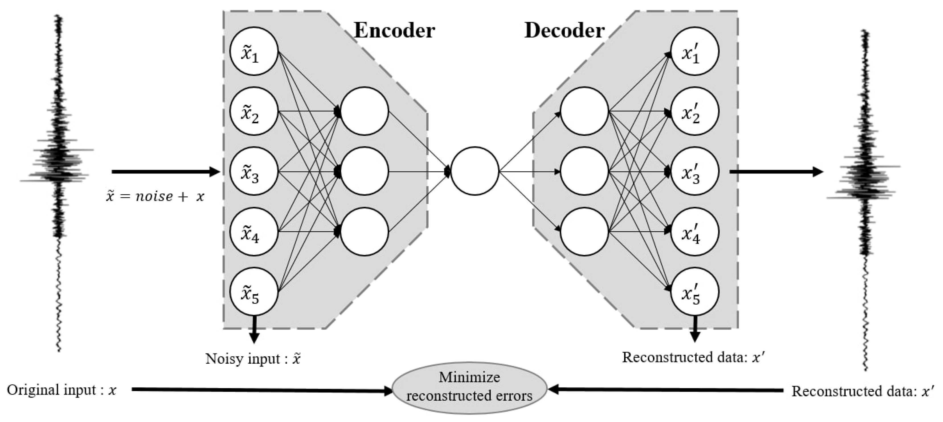
2.1. Denoising Autoencoder (DAE)

The Denoising Autoencoder (DAE) is a representative unsupervised learning-based neural network model that is widely used to remove noise from input data and extract core features of the original signal [12]. As a variant of the Autoencoder (AE), the DAE is trained by intentionally adding noise to the input data and learning to reconstruct the original signal. This process enables the model to learn robust feature representations [13].
As illustrated in Figure 1, a typical DAE consists of two components: an encoder and a decoder [12]. The encoder transforms the noisy input signal into a compressed, low-dimensional latent representation. The decoder then attempts to accurately reconstruct the original signal from this latent representation. Through this process, the DAE learns to extract features that are less affected by noise, thereby preserving only the meaningful information contained in the signal [14].
The objective function of the Denoising Autoencoder (DAE) is typically designed to minimize the Mean Squared Error (MSE) between the original input and the reconstructed output [12], as expressed by the following equation:
L x , x ^ = x x 2
where x denotes the original input signal and x represents the signal reconstructed by the DAE.
In the field of fault diagnosis using vibration data, the DAE has attracted considerable attention as a preprocessing technique that significantly improves diagnostic accuracy by removing noise and extracting key features from the data [15].

2.2. Feature Extraction

Statistical feature extraction plays a key role in distinguishing between normal and faulty states by numerically expressing various statistical properties of vibration signals [16]. Fault conditions in machinery often lead to changes in the statistical distribution of vibration signals, and utilizing representative statistical features can significantly enhance classification performance [17]. Due to their simplicity and clear interpretability, statistical features are widely adopted in vibration-based condition monitoring and fault prediction [16,18]. In this study, five statistical features were used: mean, RMS, standard deviation, kurtosis, and skewness.

2.2.1. Mean

The mean represents the overall magnitude of the signal and is defined as follows [16]:
M e a n = 1 N i = 1 N x i
where x i is the value of each data sample, and N is the total number of samples. The mean value indicates the central tendency of the data and can be used to identify balance conditions or systematic offsets in machinery.

2.2.2. Root Mean Square (RMS)

RMS is a critical feature that represents the energy or amplitude of the signal and is directly related to signal strength [18]:
R M S = 1 N i = 1 N x i 2
High RMS values often indicate the presence of mechanical faults, making it a representative indicator for condition monitoring.

2.2.3. Standard Deviation (STD)

Standard deviation quantifies the spread of the signal values around the mean and is used to assess signal volatility [17]:
S T D 1 N 1 i = 1 N ( x i x ¯ ) 2
where x ¯ is the mean of the data. A larger standard deviation implies greater signal variation and may indicate abnormalities or irregular vibrations.

2.2.4. Kurtosis

Kurtosis measures the “peakedness” of the signal distribution and is especially useful for detecting localized defects such as bearing faults [18]:
K u r t o s i s = 1 N i = 1 N ( x i x ¯ ) 4 ( 1 N i = 1 N ( x i x ¯ ) 2 ) 2
Higher kurtosis values indicate the presence of sharp peaks in the signal distribution.

2.2.5. Skewness

Skewness evaluates the asymmetry of the signal distribution and indicates whether the signal is biased in a particular direction [16]:
S k e w n e s s = 1 N i = 1 N ( x i x ¯ ) 3 ( 1 N i = 1 N ( x i x ¯ ) 2 ) 3
A skewness value greater than zero indicates a right-skewed distribution, while a value less than zero indicates a left-skewed distribution. Skewness is particularly helpful for identifying directional characteristics in fault signals.

2.3. One-Class Support Vector Machine

The One-Class Support Vector Machine (OC-SVM) is an unsupervised machine learning algorithm widely used in the fields of anomaly detection and fault diagnosis. The OC-SVM is designed to detect abnormal or faulty states by learning only from data representing normal operating conditions [19,20].
Unlike conventional Support Vector Machines, which learn from both normal and faulty classes, the OC-SVM constructs a hyperplane based solely on normal data to separate the region of normality from potential anomalies. This approach is particularly effective in industrial environments where fault data is rare or difficult to obtain [21].
As illustrated in Figure 2, OC-SVM maps input data points nonlinearly into a high-dimensional feature space and learn a hypersphere or hyperplane that maximizes the separation from the origin through the following optimization process [19].
The OC-SVM has proven to be highly effective in detecting abnormal states in machine fault diagnosis based on vibration data, as it can identify subtle differences between signal features [22]. In particular, it demonstrates high accuracy in detecting early faults and anomalies by effectively learning the decision boundary using only normal data [20,21].

3. Preliminary Study

This section presents the results of prior studies involving a DAE model trained with Gaussian noise, as well as fault diagnosis outcomes based on denoising using the Wavelet Transform. To this end, we first describe the composition of the dataset used and the preprocessing method, and then sequentially describe the structure of the model, experimental conditions, and diagnostic performance results.

3.1. Dataset

To evaluate the noise reduction performance of the DAE model depending on the type of training noise, motor load data was collected from mechanical equipment (induction motors) operated by a metropolitan railway corporation. The dataset included both normal data collected under 11 kW operating conditions and fault data representing a belt looseness condition.
From the entire dataset, 7,800,000 data points were sampled for use in the experiment. The sampling rate of the data was 4000 Hz. Examples of the normal and fault data used in the study are shown in Figure 3.
The frequency components of the data were analyzed using FFT, and the results indicated that both normal and fault signals contained significant noise in the high-frequency range above 1000 Hz, as shown in Figure 4. Based on the results of the FFT analysis, the frequency band for high-frequency noise extraction was subsequently set to 1000 Hz.

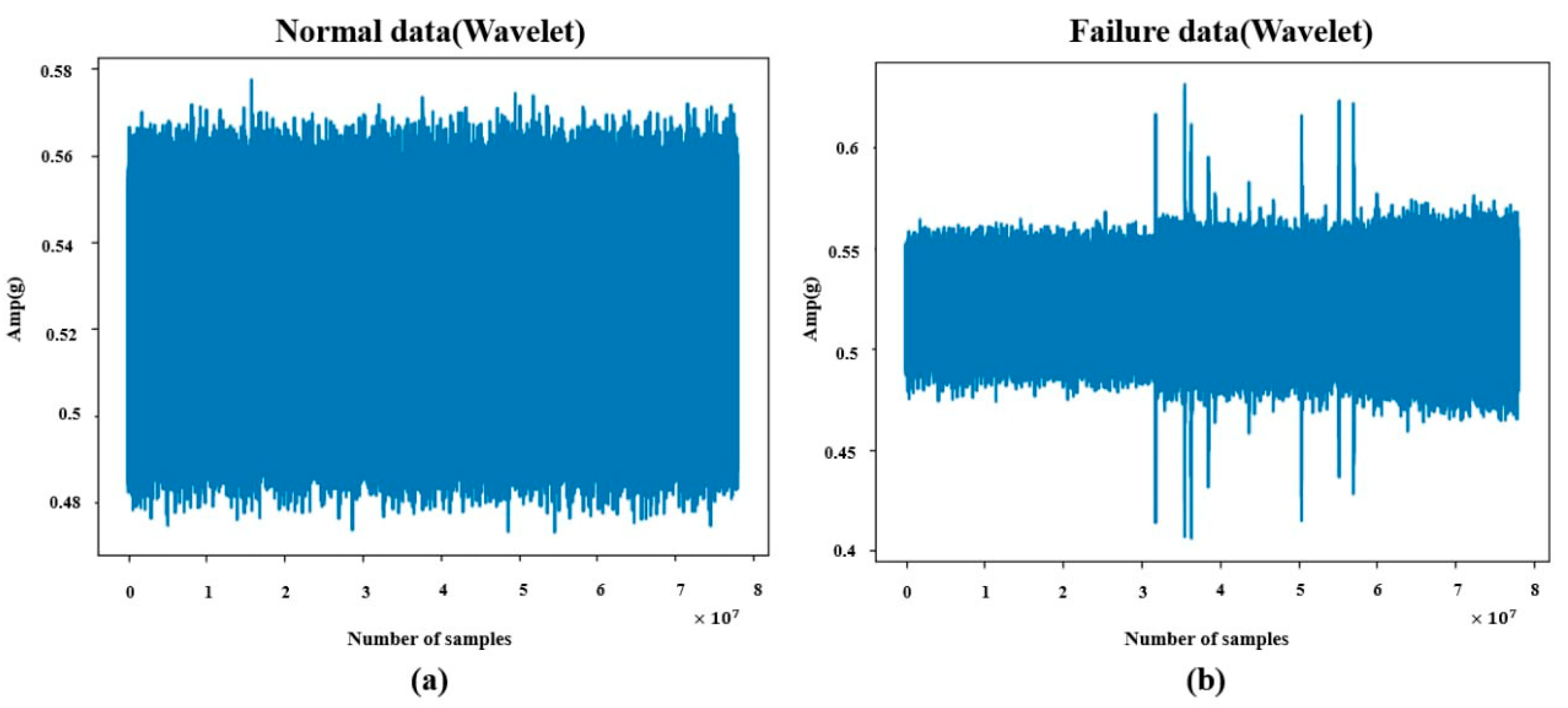
3.2. Result of Noise Reduction

This section presents the results of noise removal using a DAE model trained with Gaussian random noise. The Gaussian noise was generated with a mean of 0 and a standard deviation of 0.1, as illustrated in Figure 5. This synthesized noise was added to the raw data and used as the input to the DAE model. The encoder and decoder were structured to enable the reconstruction of the original signal from the noisy input.
To improve model stability and noise reduction performance, the data was normalized to a range between 0 and 1 during training. The denoised output obtained through the trained model is shown in Figure 6. Compared to the original raw data, the overall vibration amplitude was reduced, and the results indicate that some peak components were retained during the noise removal process.
For the preprocessing based on the Wavelet Transform, MATLAB’s Wavelet Toolbox was utilized. Given that the selection of a suitable wavelet function should reflect the characteristics of the target signal, the Daubechies 4 (db4) wavelet—known for its similarity to vibration signals—was adopted. The denoising process involved four levels of decomposition, and soft thresholding, which is commonly employed in most related studies, was applied at each level to suppress noise [23]. The resulting denoised signal is illustrated in Figure 7.

3.3. Result of Feature Extraction

Statistical feature extraction was performed on the denoised dataset comprising 7,800,000 normal and 7,800,000 fault data points. The data was divided into segments of 1000 points each, resulting in a total of 7800 segments. For each segment, five statistical features were extracted, and the results are presented in Figure 8 and Figure 9.

3.4. Result of Classification

Based on the extracted features, an OC-SVM model was trained to evaluate fault diagnosis performance. For each feature, the model was trained using only normal data to generate a hyperplane, and hyper parameter tuning was conducted to ensure that at least 90% of the normal data fell within the decision boundary (frontier). The training accuracy (Running Rate) for normal data and the fault detection rate (Failure Rate) for each feature are summarized in Table 1 and Table 2.

4. Case Study

This section presents the results of a study in which high-frequency noise components were used during the training process of the DAE model. The outcomes of this approach are compared with those of the preliminary study described in Section 3, which utilized Gaussian noise.

4.1. Result of Noise Generation

To compare the performance with the Gaussian noise-based denoising approach presented in the preliminary study, the same dataset and experimental process were used.
In alignment with the objectives of this study, high-frequency noise components from actual vibration signals were extracted by applying a high-pass filter to the raw data during the DAE training process. Figure 10 shows the extracted high-frequency components (above 1000 Hz) for both normal and fault signals. Figure 11 presents the corresponding FFT results of the extracted high-frequency noise components.

4.2. Result of Noise Reduction (Highpass)

As shown in Figure 12, the high-frequency noise components extracted using a high-pass filter were utilized during the DAE training process to remove noise from the raw data. The results of noise reduction using high-frequency noise are presented in Figure 12, and these are compared with the results obtained using Gaussian noise in Figure 5.
In the case of normal data, some peak points were suppressed; however, the overall vibration amplitude range increased significantly compared to the Gaussian noise-based model. On the other hand, for fault data, the amplitude range remained similar to that of the Gaussian noise case, and the presence of peak points was also comparable.

4.3. Result of Feature Extaction

As in the preliminary study, the data was divided into segments of 1000 samples, resulting in a total of 7800 segments. Statistical features were extracted from each segment, and the results are shown in Figure 13.
Similar to the Gaussian noise-based results, clear separation between normal and fault data was observed in three out of five features, excluding skewness and kurtosis. The most notable difference appeared in the standard deviation feature. Unlike the Gaussian noise case, which showed overlapping regions between classes, the high-frequency noise-based model demonstrated more distinct separation between normal and fault data.
In the case of kurtosis, the Gaussian noise-based features exhibited similar distributions for both classes across all segments, whereas the high-frequency noise-based results revealed some degree of distinction in specific regions.

4.4. Result of Classification (Highpass)

Following the same procedure as in the preliminary study, the OC-SVM model was trained using only normal data, with the model configured to include at least 90% of the normal data within the learned boundary. The training results and fault diagnosis rates for each feature are summarized in Table 3.
As with the Gaussian noise-based results, the training accuracy for normal data exceeded 90% across all features. The most significant improvement was observed in the kurtosis feature, where the fault detection rate increased dramatically from 26.22% to 99.5%. Although the fault detection rate for skewness decreased by approximately 27%, this reduction was relatively minor compared to the substantial gain in kurtosis. On average, models trained using high-pass noise exhibited higher fault diagnosis performance across features.

4.5. Final Comparative Analysis of Results

In this study, the F1-score was calculated to compare the noise reduction performance of the two approaches. The F1-scores for each case are shown in Table 4, Table 5 and Table 6. As previously discussed, the fault detection rate for the kurtosis feature differed significantly between the models, resulting in a higher F1-score for the high-pass noise-based model.
The average F1-scores obtained were 0.6456 for the Wavelet-based method, 0.9074 for the Gaussian noise-based DAE, and 0.9367 for the proposed high-frequency noise-based DAE. The proposed method outperformed the Wavelet approach by a margin of 0.2911 and exceeded the Gaussian noise-based model by 0.0293. Except for the skewness feature, which showed a slightly lower F1-score compared to the Gaussian noise case, the high-pass noise model achieved higher average fault detection rates and F1-scores across all features.
From a numerical perspective, an improvement of approximately 0.03 in F1-score is generally considered meaningful. In fields such as manufacturing, healthcare, and security—where accurate fault diagnosis or anomaly detection is critical—even a small gain in F1-score can provide tangible benefits. For instance, in a manufacturing setting, an improvement of 0.02 to 0.03 in F1-score can help reduce missed detections of defective products and minimize unnecessary re-inspections, thereby enhancing overall production efficiency [24].

5. Conclusions and Future Work

This study proposed a method to improve the performance of Denoising Autoencoders (DAEs), which are widely used for noise removal in image and time series data. Conventional DAE-based denoising approaches typically involve training the model with artificially added Gaussian random noise. However, Gaussian noise does not adequately reflect the complex and diverse noise patterns present in real-world vibration time series data.
To address this limitation, this study introduced a method that extracts high-frequency components from actual vibration data and uses them as training noise during the DAE learning process. To validate the proposed approach, the same feature extraction and fault classification procedures were applied as in the prior experiments using Gaussian noise and Wavelet Transform-based denoising. The final comparison results showed that utilizing high-frequency noise components led to improvements in F1-score by 0.2911 and 0.0293 over the Wavelet- and Gaussian-based methods, respectively.
These results demonstrate that, in the context of denoising vibration time series data, it is more effective to train DAE models using noise components derived from the actual data—such as high-frequency noise—rather than relying on generic Gaussian random noise.
This study has successfully demonstrated the practical effectiveness of training DAEs with noise extracted from real vibration data. The findings are expected to make meaningful contributions to the fields of predictive maintenance and condition monitoring for mechanical systems. In future work, we plan to further validate the generalizability of the proposed method using additional datasets collected from various industrial domains.

Author Contributions

Conceptualization, J.-g.J. and J.-c.L.; methodology, J.-g.J. and J.-c.L.; software, J.-g.J. and J.-c.L.; validation, J.-g.J.; formal analysis, J.-g.J.; investigation, J.-g.J. and J.-c.L.; resources, J.-g.J. and J.-c.L.; data curation, J.-g.J. and J.-c.L.; writing—original draft preparation, J.-g.J.; writing—review and editing, J.-g.J., S.-s.L., S.-Y.H. and J.-c.L.; visualization, J.-g.J.; supervision, and S.-s.L. and S.-Y.H.; project administration, J.-c.L. All authors have read and agreed to the published version of the manuscript.

Funding

This work was supported by 2025 Ministry of Oceans and Fisheries (MOF) Marine Blue Tech Future Leader Training Project ‘Training Blue Tech Leaders for Eco-Friendly Ships’ (No. RS-2025-02220459).

Institutional Review Board Statement

Not applicable.

Informed Consent Statement

Not applicable.

Data Availability Statement

Publicly available datasets were analyzed in this study. This data can be found here: https://aihub.or.kr/aihubdata/data/view.do?currMenu=115&topMenu=100&aihubDataSe=data&dataSetSn=238, (accessed on 17 January 2021).

Conflicts of Interest

Author Jun-gyo Jang was employed by the company ADIALAB. The remaining authors declare that the research was conducted in the absence of any commercial or financial relationships that could be construed as a potential conflict of interest.

References

  1. Tran, T.; Bader, S.; Lundgren, J. Denoising Induction Motor Sounds Using an Autoencoder. In Proceedings of the 2023 IEEE Sensors Applications Symposium (SAS), Ottawa, ON, Canada, 18–20 July 2023; pp. 1–6. [Google Scholar] [CrossRef]
  2. Miranda-González, A.A.; Rosales-Silva, A.J.; Mújica-Vargas, D.; Escamilla-Ambrosio, P.J.; Gallegos-Funes, F.J.; Vianney-Kinani, J.M.; Velázquez-Lozada, E.; Pérez-Hernández, L.M.; Lozano-Vázquez, L.V. Denoising Vanilla Autoencoder for RGB and GS Images with Gaussian Noise. Entropy 2023, 25, 1467. [Google Scholar] [CrossRef] [PubMed]
  3. Rubin-Falcone, H.; Lee, J.M.; Wiens, J. Denoising Autoencoders for Learning from Noisy Patient-Reported Data. In Proceedings of the Conference on Health, Inference, and Learning, Cambridge, MA, USA, 22 June 2023; Volume 209, pp. 393–409. Available online: https://proceedings.mlr.press/v209/rubin-falcone23a.html (accessed on 16 April 2025).
  4. Zhou, S.; Zha, D.; Shen, X.; Huang, X.; Zhang, R.; Chung, K. Denoising-Aware Contrastive Learning for Noisy Time Series. In Proceedings of the 33rd International Joint Conference on Artificial Intelligence (IJCAI-24), Jeju, Republic of Korea, 3–9 August 2024; pp. 5644–5652. [Google Scholar] [CrossRef]
  5. Bakir, A.; Demircioğlu, U.; Yıldız, S. A Deep Learning-Based Approach for Image Denoising: Harnessing Autoencoders for Removing Gaussian and Salt-Pepper Noises. In Proceedings of the 4th International Artificial Intelligence and Data Science Congress, Izmir, Turkey, 14–15 March 2024. [Google Scholar]
  6. Kim, K.; Lee, J. Adaptive Scheme of Denoising Autoencoder for Estimating Indoor Localization Based on RSSI Analytics in BLE Environment. Sensors 2023, 23, 5544. [Google Scholar] [CrossRef] [PubMed]
  7. Alvarado, W.; Agrawal, V.; Li, W.S.; Dravid, V.P.; Backman, V.; de Pablo, J.J.; Ferguson, A.L. Denoising Autoencoder Trained on Simulation-Derived Structures for Noise Reduction in Chromatin Scanning Transmission Electron Microscopy. ACS Cent. Sci. 2023, 9, 1200–1212. [Google Scholar] [CrossRef] [PubMed]
  8. Fang, C.; Chen, Y.; Deng, X.; Lin, X.; Han, Y.; Zheng, J. Denoising Method of Machine Tool Vibration Signal Based on Variational Mode Decomposition and Whale-Tabu Optimization Algorithm. Sci. Rep. 2023, 13, 1505. [Google Scholar] [CrossRef]
  9. Shen, H.; George, D.; Huerta, E.A.; Zhao, Z. Denoising Gravitational Waves with Enhanced Deep Recurrent Denoising Auto-Encoders. In Proceedings of the 2019 IEEE International Conference on Acoustics, Speech and Signal Processing (ICASSP), Brighton, UK, 12–17 May 2019; pp. 3237–3241. [Google Scholar] [CrossRef]
  10. Mohanty, R.K.; Soni, V.; Pradhan, P. Environmental Noise Removal from Induction Motor Acoustic Signals Using Denoising Autoencoder. arXiv 2022, arXiv:2208.04462. [Google Scholar] [CrossRef]
  11. Chen, H.; Jin, C.; Xu, Y.; Liu, F. Adaptive Denoising Autoencoder for Distance-Dependent Noise Reduction in BLE RSSI Data. Sensors 2023, 23, 5631. [Google Scholar] [CrossRef]
  12. Vincent, P.; Larochelle, H.; Lajoie, I.; Bengio, Y.; Manzagol, P.A. Stacked denoising autoencoders: Learning useful representations in a deep network with a local denoising criterion. J. Mach. Learn. Res. 2010, 11, 3371–3408. [Google Scholar]
  13. LeCun, Y.; Bengio, Y.; Hinton, G. Deep learning. Nature 2015, 521, 436–444. [Google Scholar] [CrossRef] [PubMed]
  14. Erhan, D.; Courville, A.; Bengio, Y. Why does unsupervised pre-training help deep learning. J. Mach. Learn. Res. 2010, 11, 625–660. [Google Scholar]
  15. Jia, F.; Lei, Y.; Lin, J.; Zhou, X.; Lu, N. Deep neural networks: A promising tool for fault characteristic mining and intelligent diagnosis of rotating machinery with massive data. Mech. Syst. Signal Process. 2016, 72–73, 303–315. [Google Scholar] [CrossRef]
  16. Liu, R.; Yang, B.; Zio, E.; Chen, X. Artificial intelligence for fault diagnosis of rotating machinery: A review. Mech. Syst. Signal Process. 2018, 108, 33–47. [Google Scholar] [CrossRef]
  17. Jardine, A.K.S.; Lin, D.; Banjevic, D. A review on machinery diagnostics and prognostics implementing condition-based maintenance. Mech. Syst. Signal Process. 2006, 20, 1483–1510. [Google Scholar] [CrossRef]
  18. Randall, R.B.; Antoni, J. Rolling element bearing diagnostics—A tutorial. Mech. Syst. Signal Process. 2011, 25, 485–520. [Google Scholar] [CrossRef]
  19. Scholkopf, B.; Platt, J.C.; Shawe-Taylor, J.; Smola, A.J.; Williamson, R.C. Estimating the support of a high-dimensional distribution. Neural Comput. 2001, 13, 1443–1471. [Google Scholar] [CrossRef] [PubMed]
  20. Tax, D.M.; Duin, R.P. Support vector data description. Mach. Learn. 2004, 54, 45–66. [Google Scholar] [CrossRef]
  21. Ma, J.; Perkins, S. Time-series novelty detection using one-class support vector machines. In Proceedings of the International Joint Conference on Neural Networks (IJCNN), Portland, OR, USA, 20–24 July 2003; pp. 1741–1745. [Google Scholar] [CrossRef]
  22. Widodo, A.; Yang, B.S. Support vector machine in machine condition monitoring and fault diagnosis. Mech. Syst. Signal Process. 2007, 21, 2560–2574. [Google Scholar] [CrossRef]
  23. Jang, J.G.; Noh, C.M.; Kim, S.S.; Shin, S.C.; Lee, S.S.; Lee, J.C. Vibration data feature extraction and deep learning-based preprocessing method for highly accurate motor fault diagnosis. J. Comput. Des. Eng. 2023, 10, 204–220. [Google Scholar] [CrossRef]
  24. Sokolova, M.; Lapalme, G. A systematic analysis of performance measures for classification tasks. Inf. Process. Manag. 2009, 45, 427–437. [Google Scholar] [CrossRef]
Figure 1. Denoising Autoencoder Structure.
Applsci 15 06523 g001
Figure 2. One-Class Support Vector Machine.
Applsci 15 06523 g002
Figure 3. (a) Normal data. (b) Failure data.
Applsci 15 06523 g003
Figure 4. (a) Normal data (FFT). (b) Failure data (FFT).
Applsci 15 06523 g004
Figure 5. Gaussian noise.
Applsci 15 06523 g005
Figure 6. (a) Noise reduction normal data (DAE). (b) Noise reduction failure data (DAE).
Applsci 15 06523 g006
Figure 7. (a) Noise reduction normal data (Wavelet). (b) Noise reduction failure data (Wavelet).
Applsci 15 06523 g007
Figure 8. Results of feature extraction-Gaussian noise ((a): Mean, (b): RMS, (c): STD, (d): SK, (e): KU).
Applsci 15 06523 g008
Figure 9. Results of feature extraction-Wavelet ((a): Mean, (b): RMS, (c): STD, (d): SK, (e): KU).
Applsci 15 06523 g009
Figure 10. (a) High-frequency normal data. (b) High-frequency failure data.
Applsci 15 06523 g010
Figure 11. (a) High-frequency normal data (FFT). (b) High-frequency failure data (FFT).
Applsci 15 06523 g011
Figure 12. (a) Noise reduction normal data (High-pass). (b) Noise reduction failure data (High-pass).
Applsci 15 06523 g012
Figure 13. Results of feature extraction-Highpass ((a): Mean, (b): RMS, (c): STD, (d): SK, (e): KU).
Applsci 15 06523 g013
Table 1. Results of classification (Gaussian noise).
Gaussian NoiseActual Answer
(Unit: Case)
Running
Rate
Failure
Rate
NormalFailure
Classification results by featureMeanNormal730349793.63%100%
Failure07800
RMSNormal729250893.49%100%
Failure07800
Standard DeviationNormal730050093.59%98.69%
Failure1027698
SkewnessNormal731348793.76%95.77%
Failure3307470
KurtosisNormal725454693%26.22%
Failure57552045
Table 2. Results of classification (Wavelet).
Wavelet TransformActual Answer
(Unit: Case)
Running
Rate
Failure
Rate
NormalFailure
Classification results by featureMeanNormal756523596.99%1.41%
Failure7690110
RMSNormal706673390.6%9.63%
Failure7049751
Standard DeviationNormal717768391.24%51.86%
Failure37555045
SkewnessNormal730749393.68%10.92%
Failure6948852
KurtosisNormal732347793.88%11.63%
Failure6893907
Table 3. Result of classification (High-pass).
High-Pass NoiseActual Answer
(Unit: Case)
Running
Rate
Failure
Rate
NormalFailure
Classification results by featureMeanNormal733146994%100%
Failure07800
RMSNormal717362792%100%
Failure07800
Standard DeviationNormal702977190.1%100%
Failure07800
SkewnessNormal733146994%68.6%
Failure24535347
KurtosisNormal741138995%99.5%
Failure377763
Table 4. Result of classification performance (Gaussian).
Gaussian NoisePrecisionRecallF1-ScoreF1-Score Average
FeatureMean0.93610.9670.9074
RMS0.93510.966
Standard Deviation0.9360.9860.96
Skewness0.9380.9570.947
Kurtosis0.930.5580.697
Table 5. Result of classification performance (Wavelet).
Wavelet TransformPrecisionRecallF1-ScoreF1-Score Average
FeatureMean0.9860.4960.660.6456
RMS0.9040.5010.644
Standard Deviation0.5870.36570.62
Skewness0.8960.5130.652
Kurtosis0.890.5150.652
Table 6. Result of classification performance (High-pass).
High-Pass NoisePrecisionRecallF1-ScoreF1-Score Average
FeatureMean0.9410.970.9367
RMS0.9210.958
Standard Deviation0.90110.948
Skewness0.940.7490.834
Kurtosis0.950.9950.972
Disclaimer/Publisher’s Note: The statements, opinions and data contained in all publications are solely those of the individual author(s) and contributor(s) and not of MDPI and/or the editor(s). MDPI and/or the editor(s) disclaim responsibility for any injury to people or property resulting from any ideas, methods, instructions or products referred to in the content.

