Transient Time Reduction in Time-Varying Digital Filters via Second-Order Section Optimization

Abstract

Time-varying digital filters are widely used in dynamic signal processing applications, but their transient response can significantly impact performance, particularly in real-time systems. This study focuses on reducing transient time in time-varying filters through second-order section (SOS) optimization. By employing a numerical optimization approach, we selectively adjust the coefficients of a single SOS within a higher-order filter to minimize the transient period while maintaining overall stability. Using a sequential quadratic programming (SQP) algorithm, we determine a time-varying coefficient trajectory over a finite horizon, ensuring a rapid convergence to steady-state behavior. Experimental results demonstrate that this targeted coefficient adaptation reduces transient time by up to 80% compared to conventional static designs, with minimal computational overhead. Additionally, a comparative analysis with traditional linear time-invariant (LTI) filters highlights the advantage of this method in suppressing transient oscillations while preserving long-term filter characteristics. The proposed approach provides a practical and efficient strategy for enhancing filter responsiveness in applications requiring both stability and real-time adaptability. These findings suggest that selective time variation in SOS decomposition can be a valuable tool in digital filter design, improving efficiency without excessive memory or processing demands.

1. Introduction

Digital filters are fundamental tools in signal processing, widely used in applications ranging from telecommunications and control engineering to audio engineering. Traditionally, filters are designed with fixed coefficients optimized to meet specific performance criteria such as frequency response and stability. However, in dynamic systems or time-varying environments, static filters may fail to deliver sufficient responsiveness to changing signal characteristics [1,2,3]. To address this, researchers have developed both adaptive filtering techniques—such as LMS, RLS, or Wiener filters—and time-varying filter architectures that modify filter characteristics over time [4,5,6]. Adaptive filters typically update their coefficients in real time, guided by an error signal derived from system feedback. While powerful, they are often computationally intensive and may require high memory throughput, making them less suitable for real-time or embedded systems with strict resource constraints. In contrast, time-varying filters with precomputed parameter trajectories offer a fixed, feedforward method for enhancing transient performance without incurring significant runtime/online cost.

Time-varying filters, characterized by coefficients that change over time, offer enhanced flexibility and adaptability in signal processing. Despite their advantages, time-varying filters introduce new challenges, such as increased computational complexity and potential stability issues. One critical concern is transient time—the period required for a filter to settle into its steady-state response (typically within 2%). This aspect is particularly important in real-time applications, where delays can degrade system performance. Higher-order filters, while providing better selectivity, are especially prone to prolonged transients, further complicating the design process.

This paper investigates the use of numerical optimization of second-order section (SOS) coefficients to minimize transient times in time-varying filters, offering a pathway to more efficient signal processing.

Transient time is a crucial factor in filter performance, representing the duration required for a filter to reach its steady-state response after a change in input or configuration. Additionally, a filter’s initial conditions (hot/cold start) significantly influence transient duration. In many applications, especially real-time systems, long transient times can introduce unacceptable delays, reducing overall system responsiveness and accuracy. Higher-order filters, while providing precise control over signal characteristics, often exhibit longer transient times, making their practical implementation more challenging. Reducing transient time without compromising filter stability and performance is a significant design challenge that demands innovative solutions.

The primary objective of this paper is to minimize transient time in digital filters with time-varying coefficients. To achieve this, we focus on decomposing higher-order filters into second-order sections (SOSs) to improve numerical stability and parameter control. A numerical optimization approach is proposed to fine-tune the coefficients of one or more SOSs, effectively reducing transient behavior. The goal is to strike a balance between transient time reduction and other critical performance metrics, including stability, steady-state accuracy, and memory consumption. By demonstrating the effectiveness of this method, this study aims to provide a practical framework for designing time-varying filters with improved responsiveness while maintaining efficient memory usage for storing time-varying coefficients.

2. Related Work

2.1. Literature Review

One early approach to mitigate long transients was to manipulate a filter’s initial conditions rather than its coefficients. Preloading the filter output with appropriate non-zero initial values can counteract the natural transient decay. Pei and Tseng [7] demonstrated this technique for an ECG notch filter, effectively suppressing startup oscillation in a 50/60 Hz notch by initializing the filter’s output to cancel the impulse response. Later, Kocoń and Piskorowski extended this idea by designing an FIR notch filter derived from an IIR prototype with carefully set initial conditions, achieving significant transient suppression [8]. Another method is to analytically compute the required initial outputs of internal delay elements (filter memory) for a given initial input, often by projecting the initial portion of the input signal onto the filter’s homogeneous response. Dewald et al. [9] introduced an iterative signal-shifting algorithm to automate this process. In their approach, the input signal is shifted in time and fed into the filter repeatedly, adjusting the shift until the filter’s internal memory converges to values that produce no transient. These methods treat the filter’s transient as a signal to be canceled via initial state injection.

Additionally, a more general strategy is to make the filter coefficients time-varying during the transient. Instead of keeping a fixed pole and zero configuration, the filter starts with a gentler configuration (to produce a fast decay) and then smoothly transitions to the final, more selective configuration. Piskorowski’s 2010 work introduced a Q-factor-varying notch filter where the pole radius is initially reduced (broadening the notch but damping the ringing) and then increased exponentially to the desired high Q value [10]. This approach significantly shortened the transient duration while still producing a sharp notch in steady state.

Similarly, Tan et al. [11] proposed a pole-radius variation scheme for notch filters, demonstrating transient suppression by dynamically adjusting the pole radius over time. In the low-pass filter domain, Okoniewski and Piskorowski [12] developed a time-varying IIR low-pass filter based on an analog oscillatory model. They discretized a second-order system and temporarily modulated its natural frequency and damping ratio to quickly attenuate the step-response transient. By adjusting these parameters (essentially the pole locations) during the initial response, they suppressed overshoot and reduced settling time. An iterative optimization procedure was applied to fine-tune the parameter trajectory for minimal settling time. This trend has continued in various applications, including sensing and robotics. For instance, a time-variant filter for force/torque sensors modulates its coefficients at contact onset, reducing impact force transients [13].

Gutierrez de Anda and Meza Dector [14] demonstrated a second-order low-pass filter that automatically adjusts its parameters (via a nonlinear control loop) immediately after a sudden change in the input. By momentarily widening the filter’s bandwidth and/or altering its damping factor, the filter settles much faster than a conventional static design, all while preserving the intended low-pass frequency response once the parameters revert. They also analyzed the stability of this linear time-varying (LTV) filter, showing that it maintains bounded-input bounded-output stability under the parameter adaptation scheme. Building on the idea of time-varying coefficients, de la Garza et al. [15] proposed a variational approach to design the optimal time-variation trajectory for an IIR filter’s cutoff frequency. Using calculus of variations, they derived a closed-form time-course for the filter’s pole movement that minimizes the rise time (settling time) of the step response. This optimal time-varying design achieved a shorter transient than previous ad hoc parameter variation rules, highlighting the benefit of an optimized coefficient schedule.

Amini and Mozaffari Tazehkand [16] recently presented a feedback-structured IIR notch filter with transient suppression achieved by continuously varying the feedback gain. In their design, the pole radius (which determines the notch sharpness and transient length) is kept lower than its final value at the moment of filter startup, thus damping the initial response. Sharma et al. [17] took a similar time-varying approach by leveraging a lattice wave digital filter structure for the notch. Their lattice notch filter begins with a relatively wider notch (lower Q) and progressively reduces the notch bandwidth as time advances, effectively shortening the ringing duration. The lattice wave digital implementation ensures numerical robustness and was shown to produce minimal transient overshoot, which the authors validated through FPGA implementation results.

In addition to time-varying strategies, there are also design-time techniques to improve notch filter performance. Jayant et al. [18] pursued a minimax optimization approach for a fixed-coefficient notch filter targeting 50 Hz noise in ECG. By formulating the filter design as an optimization problem, they adjusted the pole-zero locations to minimize the worst-case error between the desired ideal notch response and the realized filter response.

Introducing time variation in filter coefficients raises important stability considerations. In linear time-invariant (LTI) filters, stability is assured by having all poles inside the unit circle (for discrete-time filters). With time-varying filters, however, poles move over time and traditional LTI stability criteria no longer directly apply [19,20].

Kamen’s work [21] introduced an algebraic theory of poles and zeros for linear time-varying systems, providing a groundwork for understanding how system eigenvalues generalize in the time-varying case. This framework helped define notions of “instantaneous” poles or spectral values that evolve with time, which is critical for discussing stability beyond the static pole locations of LTI systems. Notably, Zhu [22] presented a necessary and sufficient criterion for exponential stability of linear time-varying (LTV) discrete-time systems.

Recent studies have extended time-varying filter techniques across various domains. For instance, Ye and Song [23] embed a command filter with time-varying gain into a backstepping control scheme, simplifying the controller design for high-order systems while preserving prescribed transient performance. Jelfs et al. [24] develop an adaptive all-pass filter to track nonstationary propagation delays, employing an LMS-style coefficient update that continuously adjusts a filter’s parameters for accurate time-varying delay estimation. Furthermore, Wu et al. [25] introduce a novel time-varying filtering algorithm based on a short-time fractional Fourier transform with time-dependent transform order, achieving effective filtering of multi-component signals whose spectral characteristics change over time.

In addition to these algorithmic developments, time-varying filters have proven effective in specific applications. Cui et al. [26] present a Kalman filtering approach for bearing prognostics in which the filter’s dynamics evolve with the system’s degradation state, allowing the model to automatically adapt across different wear stages and improve remaining-life prediction accuracy. Similarly, in the audio domain, Chilakawad and Kulkarni [27] implement time-varying IIR filtering in binaural hearing aids to accommodate device nonlinearities and dynamically changing acoustic environments, illustrating the broad applicability of time-varying filter design in diverse real-world systems.

2.2. Gap Identification

A key challenge in the current state-of-the-art design of time-varying filters is the flexibility of transient time. In this paper, we shift the focus to another practical aspect of these techniques: the memory consumption required to store time-varying parameters. Previous studies have proposed selecting coefficient sets in a way that allows parameter values to be approximated using simple curve-fitting techniques, reducing the need for extensive storage.

This paper introduces an alternative approach to selecting coefficients, aiming to achieve efficient transient time reduction while minimizing memory usage. Specifically, the method focuses on optimizing a single section within a decomposed higher-order digital filter, balancing transient performance with reduced storage requirements.

3. Materials and Methods

3.1. Time-Varying Filters

The concept of time-varying coefficients has primarily been explored in the context of adaptive filtering techniques, where the filter’s coefficients evolve over time to address specific problems or align with the chosen method. In this work, we propose using a predefined control rule to achieve the fastest possible response from the equalized filter while preserving its long-term frequency characteristics. Unlike adaptive filtering, our approach involves calculating the control rule once during the design phase, allowing it to be applied consistently whenever a relevant excitation occurs. The difference equation of a digital linear time-variant system (LTV) can be written as follows:

$$y \left[n\right]={\sum }_{k=1}^M{a}_k\left[n\right]·y\left[n-k\right]+{\sum }_{k=0}^N{b}_k·x\left[n-k\right],$$

(1)

where

$M$—The number of previous outputs $\left(y\left[n-k\right]\right)$ included in the equation.

$N$—The number of current and previous inputs $\left(x\left[n-k\right]\right)$ considered.

$a_k\left[n\right]$—Time-varying coefficients for the feedback terms (previous outputs).

$b_k\left[n\right]$—Time-varying coefficients for the feedforward terms (inputs).

$y\left[n\right]$—Current output at time step $n$.

$x\left[n\right]$—Current input at time step $n$.

3.2. Transient Behavior Analysis

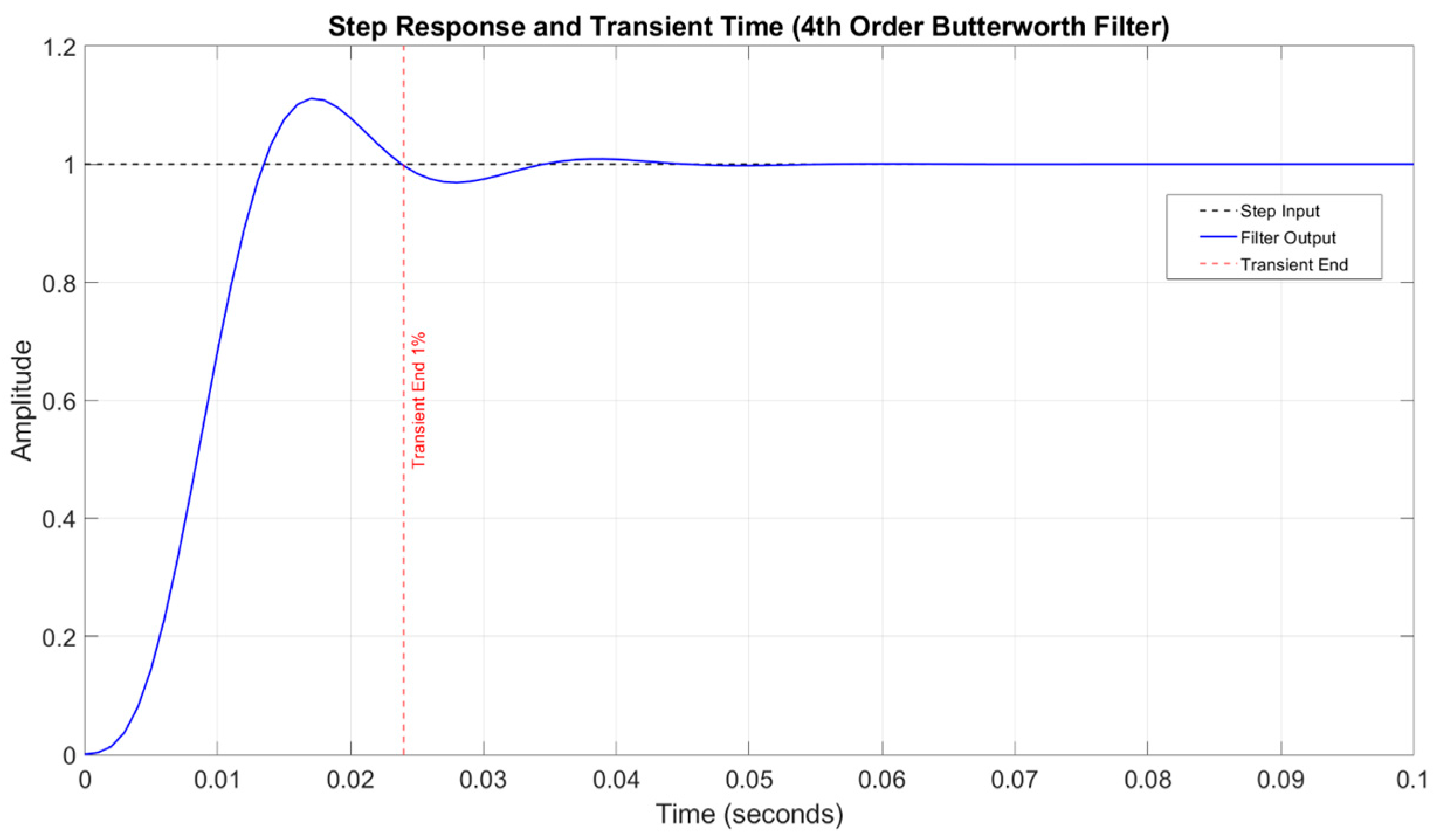
Transient time in digital filters is the interval required for the filter’s output to stabilize after a sudden change in the input signal, such as a step input. The duration of the transient response is influenced by the filter’s parameters, including the pole locations, which dictate stability and speed of convergence. Poles closer to the unit circle in the z-plane lead to longer transient times, as the system response decays more slowly. Additionally, the filter order is a significant factor. Higher-order filters typically produce more complex and extended transient behaviors due to the interplay of multiple poles and zeros.

Figure 1 depicts an exemplary step response of the 4th-order low-pass Butterworth filter. The measured 1% steady-state transient time has settled at 0.024 s after step excitation.

Figure 1. Step response and transient time of an exemplary 4th-order low-pass Butterworth filter (sampling frequency Fs-1 kHz; cutoff frequency Fc-50 Hz).

Time-varying coefficients can further complicate transient behavior, introducing variability that may prolong or destabilize the response, underscoring the need for careful parameter optimization.

3.3. Second-Order Section Decomposition

Higher-order digital filters often encounter numerical challenges, such as coefficient quantization sensitivity and overflow, which can degrade performance in low-precision or fixed-point implementations. By decomposing the filter into multiple second-order sections (SOS), these numerical issues are localized and thus more effectively mitigated. Each SOS is represented as a biquad transfer function:

$$H(z)={\displaystyle \frac{b_0+b_1{z}^{-1}+b_2{z}^{-2}}{1+a_1{z}^{-1}+a_2{z}^{-2}}}.$$

(2)

This corresponds to the time-domain difference equation:

$$y\left[n\right]=-a_{1}y[n-1]-a_{2}y[n-2]+b_{0}x\left[n\right]+b_{1}x[n-1]+b_{2}x[n-2].$$

(3)

A higher-order IIR filter of order N is typically realized by cascading $M=\left[{\displaystyle \frac{N}{2}}\right]$ second-order sections, with an optional first-order section for odd-order filters:

$$H_{total}(z)={\prod }_{i=1}^M{H}_i\left(z\right).$$

(4)

The decomposition into SOS format is commonly performed using polynomial factorization of the filter’s numerator and denominator.

SOS, with its fewer coefficients and simpler pole-zero structure, is less susceptible to instability and rounding errors. This modular design facilitates targeted optimization, as each second-order section can be tuned independently for optimal performance, reducing the overall computational effort. From a resource perspective, SOS decomposition lowers memory usage and power consumption, making it particularly valuable for real-time and embedded systems. It also enhances flexibility by allowing sections that handle more critical frequency components to use higher-precision resources as needed. Moreover, the ability to add or remove sections without overhauling the entire filter design increases scalability—an important benefit in adaptive or time-varying scenarios where filter parameters may need to change rapidly. Ultimately, SOS decomposition provides a robust framework for achieving high filter performance, efficient resource utilization, and straightforward optimization in higher-order digital filter designs.

In this paper one can find an extension of the benefits of using SOS decomposition in terms of a proposal to introduce time-varying coefficients into a finite horizon to improve the transient time of the whole design.

3.4. Decomposition Approach

Decomposing a higher-order digital filter into second-order sections (SOSs) provides a stable and numerically efficient means of realizing the transfer function. In this work, we use 2023b MATLAB’s built-in function, which takes the filter’s numerator and denominator polynomials (in transfer function form) and factors them into multiple second-order blocks. Each block corresponds to a pair of conjugate poles (and zeros), thereby reducing sensitivity to rounding errors and making it straightforward to manage overflow concerns. We opt for a cascade structure since it simplifies the allocation of scale factors for each block, ensuring a more uniform distribution of gain and helping maintain stability. Moreover, by breaking the filter into multiple SOSs, we can individually optimize or tweak specific sections as needed, offering flexibility for further performance refinements without rewriting the entire filter design.

Figure 2 presents the magnitude response of the full 6th-order low-pass elliptic filter (sampling frequency Fs-1 kHz; cutoff frequency Fc-100 Hz; passband ripple Rp-1dB; stopband attenuation Rs-40dB) and the magnitude responses of the three second-order sections.

Figure 2. Magnitude responses: 6th-order low-pass elliptic filter decomposition.

Figure 3 depicts the step responses of the full and SOS decomposition of the same low-pass elliptic filter.

Figure 3. Step responses: 6th-order low-pass elliptic filter decomposition.

We propose to drive the focus to one of the sections and apply the time-varying coefficient methodology to reduce the transient time of the whole design.

3.5. Numerical Optimization

We focus on optimizing a single second-order section (SOS) whose time-varying difference equation can be expressed as in (3), where $a_k\left[n\right]$ and $b_k\left[n\right]$ are the time-varying coefficients for $k\in \mathrm{0,1},2$. Over a finite horizon H, these coefficients are allowed to vary from sample to sample, while for $n>H$ they revert to their stationary values, which ensures long-term stability. The objective function is formulated to minimize the transient response by penalizing deviations of the filter output $y\left[n\right]$ from a desired steady-state target $y_{ss}$ during the initial H samples:

$$J\left(\theta \right)={\sum }_{n-1}^H{\left(y\left[n;\theta \right]-y_{ss}\right)}^2,$$

(5)

where

$$\theta =\left\{a_1\right[n],a_2[n],b_0[n],b_1[n],b_2[n] | n=1,... ,H\},$$

(6)

collectively represents all time-varying coefficients $a_k\left[n\right]$ and $b_k\left[n\right]$ for $1\le n\le H$. The cost function $J\left(\theta \right)$ encodes the principle that the filter output should converge as quickly as possible to $y_{ss}$, thereby reducing transient state. Additionally, a set of stability constraints ensures that the time-varying SOS stays a valid candidate. One can find further details about time-varying filter stability in the author’s previous works. To solve this constrained minimization problem, we employ the Sequential Quadratic Programming (SQP) algorithm for its robust handling of nonlinear constraints. We have also proposed a bounding constraint in the form of

$$-1\le a_k\left[n\right],b_k\left[n\right]\le 1,$$

(7)

which is a simple yet effective means to prevent runaway filter gains that might otherwise prolong or destabilize the transient.

Once optimized, the coefficient set is stored and used in real-time operation during known transient events (e.g., a step input or signal onset). After H samples, the coefficients revert to their stationary (LTI) values:

$$a_i[n]=a_i^{LTI}[n], b_i[n]=b_i^{LTI}[n] \mathrm{f}\mathrm{o}\mathrm{r} n>H,$$

(8)

This hybrid approach maintains the filter’s desired long-term frequency response while minimizing initial settling time.

4. Results

4.1. Optimization Outcomes

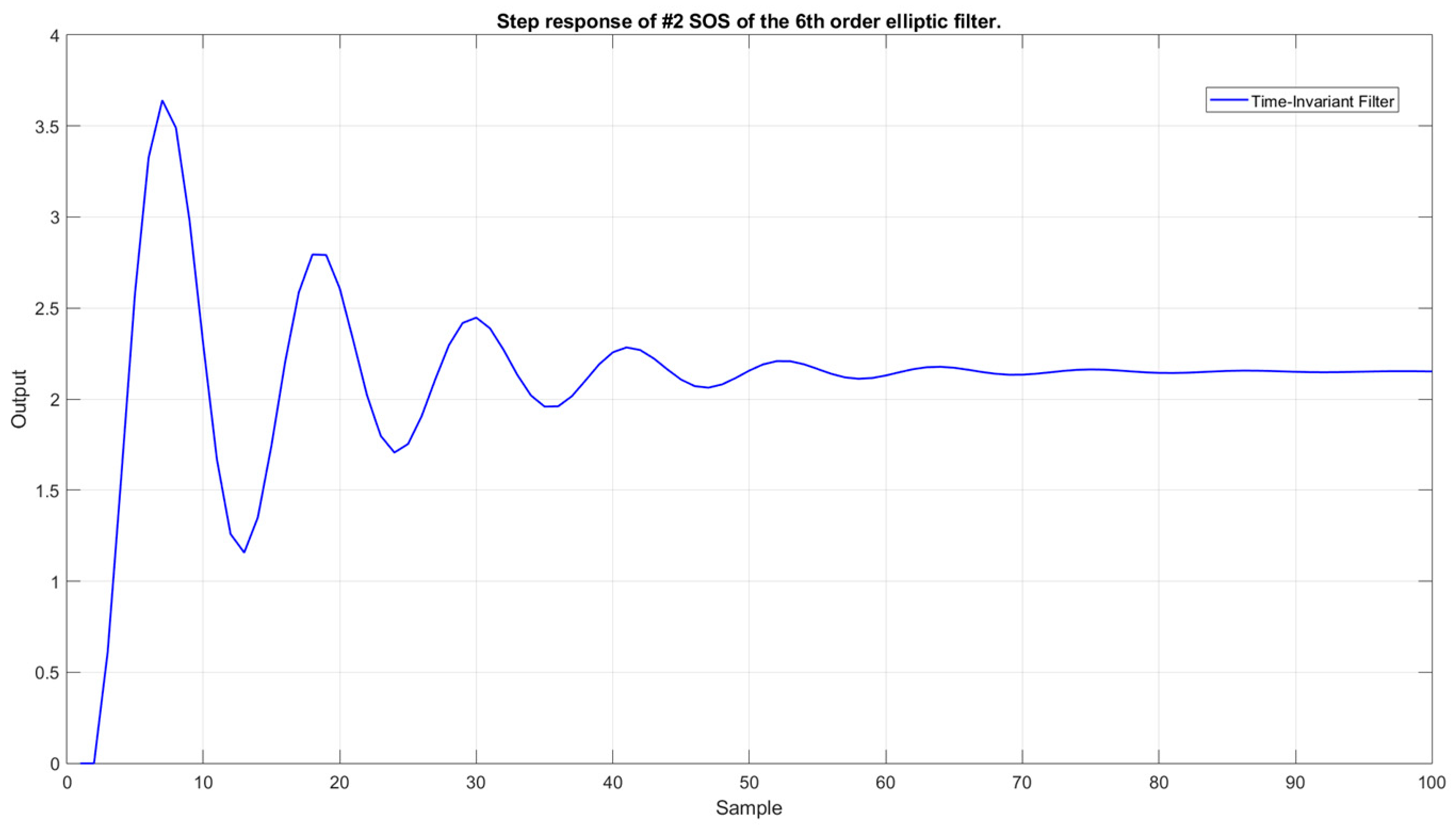
As an example let us use the elliptic filter mentioned in Section 3.4. Figure 4 presents the step response of #2 SOS of the final design.

Figure 4. Step response of #2 SOS of the 6th-order elliptic filter.

Table 1 presents the coefficients of the stationery #2 SOS.

Table 1. Linear time- invariant coefficients of the #2 SOS.

Coefficients	0	1	2
a	1	−1.58314580285905	0.867241363463590
b	1	−1.38888837010072	1

Table 2 outlines the performance of the section in terms of transient time duration.

Table 2. Transient time data for classical stationary SOS.

Transient Time Threshold	Sample Index	Time
1%	54	0.053 s
2%	47	0.046 s
5%	31	0.03 s

As one can notice, this section’s step response is characterized by significant ripple behavior.

By introducing the iterative SQP solver described in Section 3.5, we have acquired a new time-varying SOS with a significantly improved transient time. Table 3 and Table 4 present the set of coefficients ($a_k\left[n\right]$ and $b_k\left[n\right]$) that change in the span of five samples (horizon).

Table 3. Time-varying set of $a_k\left[n\right]$ coefficients.

Sample	${\mathit{a}}_0\left[\mathit{n}\right]$	${\mathit{a}}_1\left[\mathit{n}\right]$	${\mathit{a}}_2\left[\mathit{n}\right]$
n = 1	1	0.1058	−0.0093
n = 2	1	0.1097	0.5325
n = 3	1	0.1595	0.4362
n = 4	1	0.3704	0.2778
n = 5	1	−1	0.6328

Table 4. Time-varying set of $b_k\left[n\right]$ coefficients.

Sample	${\mathit{b}}_0\left[\mathit{n}\right]$	${\mathit{b}}_1\left[\mathit{n}\right]$	${\mathit{b}}_2\left[\mathit{n}\right]$
n = 1	0.9727	0.5254	0.6714
n = 2	0.1920	0.5303	0.7413
n = 3	0.5733	0.7991	0.7783
n = 4	0.9613	0.991	0.9952
n = 5	0.4464	0.4646	0.4498

As mentioned in Section 3.5, after reaching the horizon (five samples) the coefficients settle on the original #2 SOS parameters to preserve the desired frequency characteristic. Figure 5 outlines the graphical comparison of the LTI and LTV #2 SOS instances.

Figure 5. Comparison of step responses of the #2 SOS designed with classical methodology and the proposed time-varying approach.

Table 5 summarizes the improvement in the reduction in the transient time by using the time-varying coefficients.

Table 5. Transient time data for time-varying SOS.

Transient Time Threshold	Sample Index	Time
1%	3	0.02 s
2%	3	0.02 s
5%	3	0.02 s

4.2. Comparison with Baseline

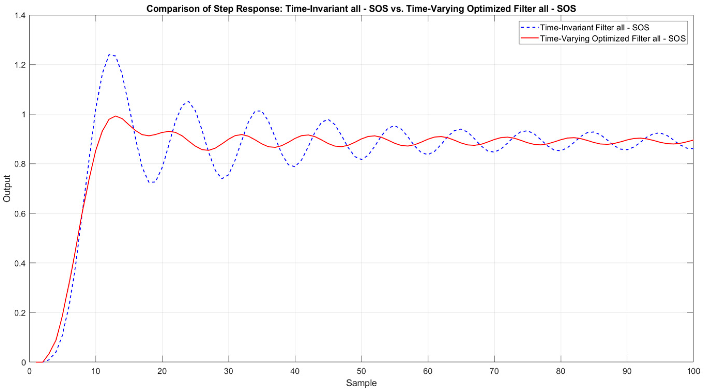
The previous section proved the usefulness of the time-varying concept in terms of reducing the transient time of one of the second-order sections. For the whole design to be useful, one needs to focus on the performance of the final (full) filter design. Figure 6 presents the comparison of the complete static solution with the novel approach to improving one of the SOS parts.

Figure 6. Comparison of full classical time-invariant filter with the novel design with one time-varying SOS.

Figure 6 compares the step responses of a time-invariant, SOS-based digital filter (blue dashed line) with a time-varying, SOS-based design (red solid line). The baseline refers to a standard sixth-order elliptic filter, implemented using three fixed second-order sections. All coefficients remain constant over time, and no transient optimization is applied. In the proposed LTV design, the same sixth-order elliptic filter structure is used, but only one SOS (#2) has its coefficients varied across five samples based on the SQP-optimized trajectory. The other two SOSs remain identical to those in the baseline. Notably, the time-varying filter converges more rapidly to the steady-state level, displaying less overshot and fewer oscillations during the early samples. This outcome underscores the advantage of selectively adjusting SOS coefficients to reduce unwanted oscillations and accelerate the settling process, reducing the transient time of the filtering structure. Table 6 summarizes the overall improvement in the reduction in the transient time of the complete design when compared to the classical time-invariant structure.

Table 6. Transient time comparison between classical (LTI—linear time-invariant) and the proposed (LTV—linear time-varying) method.

Transient Time Threshold	Sample Index (LTI)	Time (LTI)	Sample Index (LTV)	Time (LTV)
1%	198	0.197 s	118	0.117
2%	176	0.175 s	68	0.067
5%	86	0.085 s	16	0.015

As one can notice, the reduction in the transient time has reached up to 80% for the 5% threshold, which should be considered a major improvement.

4.3. Robustness Analysis

A natural way to highlight the benefits of introducing time-varying coefficients into a single second-order section is to compare how both the classical, fully LTI filter and the partially time-varying design perform under changing signal conditions. Specifically, analyzing their time-domain behavior when subjected to different noise levels or varying signal frequencies provides clear evidence of how transient response and overall performance are impacted. By overlaying their outputs on a noisy input signal, one can observe which approach settles faster and better suppresses undesired oscillations. This direct, side-by-side comparison helps quantify whether allowing even a single SOS can significantly reduce the transient period without degrading the filter’s long-term characteristics.

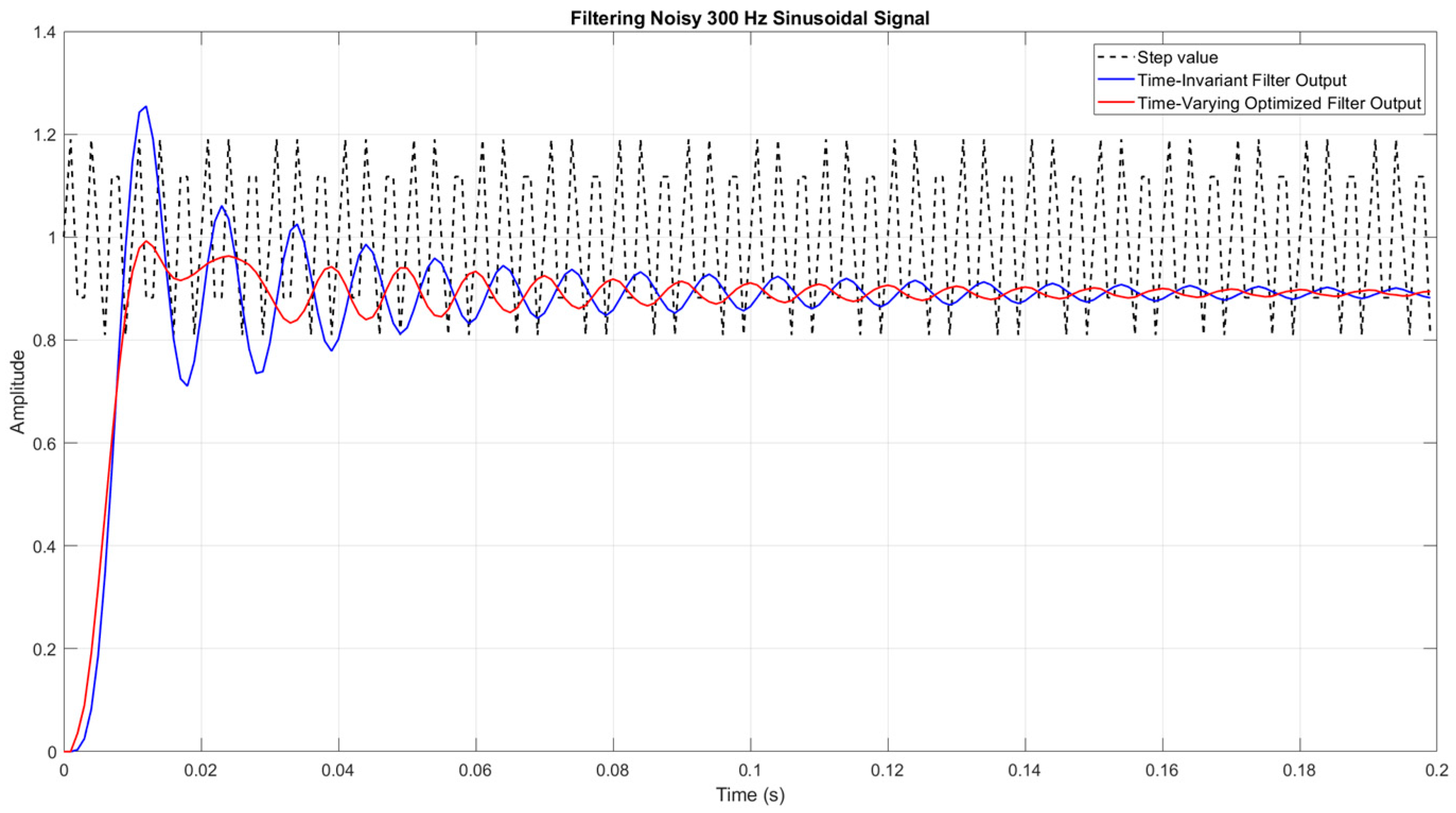
Figure 7 illustrates an exemplary performance of both the classical and the proposed structures within a noised environment.

Figure 7. Classical linear time-invariant filtering structure compared with proposed linear time-varying SoS on exemplary test signal.

In the first experiment, we added a high-frequency (300 Hz) noise component on top of an otherwise simple step input signal. The dashed black trace in Figure 7 shows how the noise significantly distorts the step’s clean rise. A conventional time-invariant filter (blue line) reduces much of the noise but still exhibits a notable transient, including an overshoot and oscillations as it settles. By contrast, modifying a single second-order section to have time-varying coefficients (red line) shortens the settling period while maintaining effective noise suppression. This illustrates how the proposed approach can outperform a purely LTI filter when faced with strong high-frequency interference.

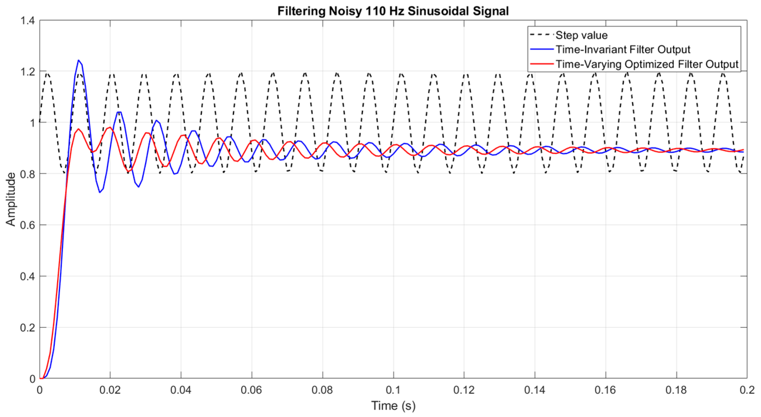
To further evaluate the robustness of the proposed method, we examined a more challenging case where the interfering signal lies just above the passband of the elliptic filter. Specifically, we added a 110 Hz sinusoidal component—which is only 10 Hz above the cutoff frequency of the sixth-order low-pass elliptic filter (Fc = 100 Hz)—to a step signal. This setup stresses the filter’s ability to suppress high-frequency content close to the transition band, while still preserving a rapid transient response.

Figure 8 illustrates an exemplary performance of both the classical and the proposed structures within a challenging noised environment.

Figure 8. Comparison of classical time-invariant filter and proposed time-varying SOS filter under step input with added 110 Hz interference. The 110 Hz component lies just above the 100 Hz cutoff, creating a near-edge suppression challenge. The time-varying design shows faster and cleaner convergence.

As shown in Figure 8, the classical time-invariant filter (blue) exhibits a relatively slow settling behavior with noticeable oscillations caused by the nearby frequency interference. In contrast, the proposed design with one time-varying SOS (red) converges more quickly and cleanly, effectively dampening the transient while maintaining similar steady-state accuracy. This result highlights the method’s strength in handling tight spectral proximity scenarios, which are common in dense signal environments.

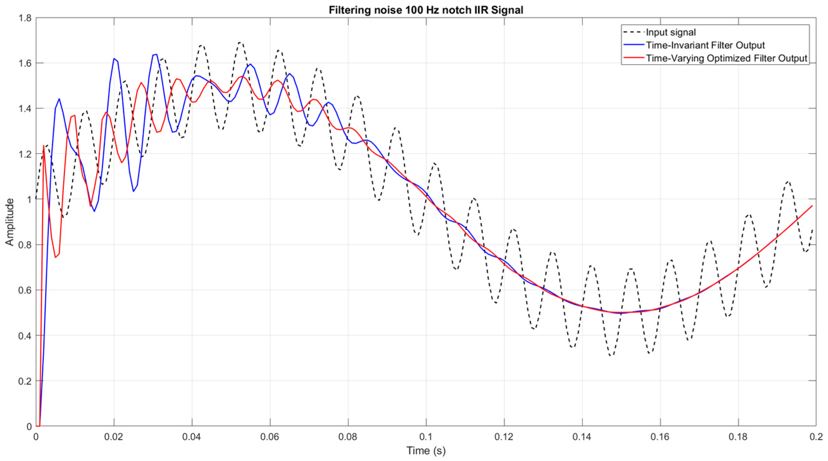
Figure 9 presents the classical notch-type IIR filter compared to another implementation of the proposed method.

Figure 9. Comparison of a classical IIR notch filter with the proposed time-varying methodology.

In this experiment, we employ an IIR notch filter designed to attenuate a 100 Hz disturbance while preserving both the step component and any relevant lower frequencies. The dashed black curve again shows the input signal, now containing a step, a 5 Hz “useful” component, and strong 100 Hz noise. The notch filter’s time-invariant version (blue) substantially reduces the 100 Hz amplitude but still suffers from a longer transient and overshoot. By allowing one second-order section to have time-varying coefficients (red), the filter settles faster and more cleanly, with less oscillatory behavior. These results demonstrate that the proposed time-varying SOS technique can be seamlessly integrated into notch-type IIR filters, enabling them to reduce transient times while maintaining precise attenuation at the targeted notch frequency.

5. Discussion

In this study, we found that introducing time-varying coefficients into only one second-order section can substantially shorten the overall transient time, offering a clear advantage over a fully time-invariant design. At the same time, the computational overhead remains relatively modest, since the method requires storing just a limited set of coefficients within a user-defined horizon rather than adapting the entire filter for the time-varying concept. These optimized coefficients, derived through a nonlinear routine that carefully balances settling speed and stability, cannot be readily approximated by a simple mathematical function or curve, so the most reliable approach is to store them directly. Although this adds some memory usage—particularly in low-power or embedded contexts—its footprint is still far smaller than that of a fully time-varying filter architecture. By confining the mechanism to one SOS, the structure preserves the benefits of time-varying behavior exactly where it is most needed, while leaving the rest of the filter in a low-complexity, stationary form. Moreover, empirical tests confirm that this targeted approach preserves steady-state performance across a range of signal and noise conditions. Thus, it provides a practical middle ground, allowing significant transient improvements in return for only a slight increase in storage and computational effort.

Although the approach of using time-varying coefficients in one second-order section has demonstrated notable benefits, it is not universally advantageous across all filter structures or use cases. For instance, Butterworth filters, with their relatively low selectivity, gain much less from this technique, suggesting that filters offering sharper roll-offs or more complex pole-zero placements stand to benefit most. Additionally, while the coefficient adaptation process proves straightforward under a “cold start,” where the filter begins with zero initial conditions, the performance in a “hot start” scenario—when the filter is already operating—requires further investigation. Another critical concern is determining the precise moment at which to initiate time-varying behavior; if it is triggered too early or too late, the potential gains can be diminished or overshadowed by unnecessary overhead. Likewise, rapid changes in the input signal, such as narrow “stairs,” can disrupt the predefined horizon if the filter coefficients are only optimized for a single transient event. These issues underscore the method’s current limitations and highlight areas where additional research—on trigger mechanisms, adaptive horizons, and robust designs for rapidly shifting signals—remains necessary.

6. Conclusions

In this paper, we introduced a novel method for introducing time-varying coefficients into a single second-order section (SOS), thereby reducing transient times without incurring excessive computational overhead. By selectively adapting only one SOS, we strike a balance between fully time-varying filtering and a purely static approach. Our analysis indicates that filters with sharper roll-offs, such as elliptic or Chebyshev designs, derive the most significant benefits, although even low-selectivity filters show moderate improvements. Practical demonstrations revealed a pronounced reduction in settling time under varying noise levels and signal conditions, underscoring the technique’s robustness. We also highlighted the importance of carefully choosing the horizon and triggering mechanism to maximize performance gains. Overall, our findings confirm that a selective time-varying strategy can markedly enhance responsiveness while preserving the filter’s stability.

The time-varying SOS strategy has immediate relevance in scenarios demanding both rapid settling and stable operation, such as live audio signal processing and real-time communication systems. By reducing the filter’s transient period, latency-sensitive applications—like wireless data transmission, virtual reality audio rendering, and adaptive control systems—can benefit from quicker responsiveness. Automotive sensor fusion is another promising domain, where faster convergence aids in smoother integration of rapidly updated sensor inputs. The method’s targeted adaptation also suits power-constrained embedded devices that need to optimize transient behavior without expending excessive computational resources. Finally, its flexibility and moderate complexity make it a practical choice for any system where short-lived disturbances must be addressed quickly while maintaining robust long-term performance.

Future work will involve refining the triggering mechanism for time-varying updates, especially in “hot start” scenarios where the filter has already been operating. Another promising line of research is to develop dynamic or adaptive horizons that better handle signals with narrow “stairs” or sudden changes. Extending this partial adaptation strategy to higher-order or multidimensional filters also merits investigation, as it may open doors to more sophisticated applications like 3D audio or MIMO communication systems. Real-time implementation is equally important, ensuring that the computational overhead of coefficient updates remains feasible for embedded and low-power devices. Finally, an in-depth exploration of the cost–benefit balance between the extra memory needs for storing time-varying parameters and the performance gains in transient reduction can guide practical design choices.