Abstract
In planar linkage mechanisms, due to various influencing factors, the existence of joint clearance becomes an inevitable phenomenon, which substantially diminishes the precision of the system’s movement. Currently, the majority of studies are largely confined to simple mechanisms with a single clearance, whereas investigations into more intricate systems with multiple types of clearances are still lacking. In view of this, this paper proposes an innovative dynamic algorithm for complex multilink mechanisms, aiming to deeply explore the specific impacts of multiple factors on dynamic response and nonlinear rigid-body properties, as well as its reliability analysis. Taking an eight-bar mechanism as an example, a dynamic model with mixed clearances is constructed, based on which the dynamic responses of the mechanism to different types of clearances are studied. Simultaneously, the effects of different variation ranges of clearance values and traveling speeds on the dynamic response, nonlinear characteristics, and dynamic accuracy reliability analysis of the mechanism were investigated. This research not only lays a robust theoretical foundation for the dynamics of multilink mechanisms but also demonstrates significant value and significance in both academic research and engineering application fields.
1. Introduction
With the swift economic advancement, the machinery manufacturing sector is steadily evolving towards greater speed, enhanced precision, and increased productivity. The mechanical system’s functionality and efficiency are critically dependent on the mechanism, which is essential for its overall operation. Therefore, the study of mechanism dynamics is of considerable practical significance and has a significant impact on the development of the manufacturing industry. Among these mechanisms, multilink mechanisms, serving as critical components, have found extensive applications across a variety of fields, including medical devices, mobile robotics, aerospace, agricultural machinery, and compression equipment, garnering considerable attention and in-depth investigation from scholars. In multilink mechanisms, various components are interconnected through revolute and prismatic joints. Yet, due to factors like manufacturing tolerances, installation inaccuracies, and friction losses, clearances often arise in the kinematic pairs. Clearances can result in adverse interactions among the kinematic pairs, substantially impacting precision and stability of the mechanism’s movement [1,2,3,4,5,6,7,8,9]. So, it is crucial to conduct comprehensive study on the dynamic behaviors of multilink mechanisms, particularly those with mixed clearances.
Many mechanisms in the real world consist of one or more revolute joints, which are essential for their proper functioning. However, the existence of clearances in these joints causes discrepancies between ideal and actual motion of the mechanisms. Therefore, investigating the effects of clearances in revolute joints is of significant importance for understanding and improving the performance of such systems. Tan et al. [10] employed the Newton–Euler equation system to establish a dynamics model for a slider-crank mechanism with multiple rotary joint clearances, aiming to explore impact of these clearances of the mechanism’s performance. Olyaei et al. [11] constructed a corresponding rigid body dynamics model for a sliding crank mechanism with a single rotary joint clearance and further proposed a stabilization control strategy based on the Pyragas principle. Zheng et al. [12] utilized finite element analysis to discretize slider components in a multibody system and conducted an in-depth study on deformation characteristics of slider in a slider-crank system with clearances. Zheng et al. [13] integrated the Absolute Nodal Coordinate Formulation (ANCF) with finite element analysis to build a dynamics model that comprehensively considers bearing stiffness, joint clearance, and flexible links, and used this model to predict the dynamic accuracy of high-speed stamping mechanisms. Lu et al. [14] constructed a six-DOF vehicle shimmy dynamics model incorporating multiple clearances and deeply explored the specific impact of clearance factors on vehicle shimmy response. By analyzing phase diagrams and Poincaré section maps, they revealed the presence of chaotic dynamic behavior in this vehicle shimmy system. Yu et al. [15] comprehensively investigated the dynamic characteristics of an over-constrained planar parallelogram mechanism with revolute joint clearances, focusing on influences of these clearances on mechanism’s dynamic performance. Farahan et al. [16] selected a planar 4-bar mechanism with a single revolute joint clearance as a case study and constructed a dynamics model based on the second kind of Lagrange’s equations. They thoroughly investigated the influence of revolute joint clearances on nonlinear dynamic properties of mechanism by examining phase plane diagrams, Poincaré maps, and bifurcation diagrams. Hou et al. [17] selected the RU-RPR mechanism, taking into account the clearances in revolute joints, and analyzed its chaotic behavior through phase portraits, Poincaré maps, and the highest Lyapunov exponent. Wang et al. [18] conducted an in-depth investigation of the nonlinear dynamics of a rigid-flexible coupling slider-crank mechanism with rotary joint clearances, utilizing phase plane diagrams, Poincaré section maps, and bifurcation diagrams. Erkaya et al. [19] conducted a comparative analysis focusing on the differences in dynamic responses between rigid sliding crank mechanisms and rigid-flexible coupling slider-crank mechanisms with revolute joint clearances. They used ADAMS software for simulation to verify the accuracy of their theoretical analysis.
The prismatic joint is an indispensable component in mechanism construction and a crucial factor for realizing and transmitting the intended functions of a mechanism. More complex mechanisms require more prismatic joints to achieve their functional requirements. The stability and accuracy of prismatic joints significantly impact the performance of the mechanism. Thus, examining mechanisms with prismatic joint clearance is of significant importance. Flores et al. [20] developed and elaborated a new dynamic modeling method for crank-slider mechanisms with prismatic joint clearance based on the theoretical framework of nonsmooth dynamics. They conducted an in-depth analysis of how prismatic joint clearance impacts kinematic and dynamic properties of these systems. Megahed et al. [21] adopted the Lankarani–Nikravesh (L-N) model framework to establish dynamic equations for a slider-crank mechanism with clearance. They comprehensively analyzed the specific influence of velocity factors on the dynamic behavior of this mechanism. Qian et al. [22] constructed a 3D geometric representation of a prismatic joint with clearance and thoroughly investigated nonlinear dynamic properties of the system using numerical analysis, simulations, and experimental validation. Skrinjar et al. [23] conducted modeling analysis for pin-groove joints with clearance and thoroughly investigated the influence of various kinematic constraints and contact force models on the dynamic characteristics of the mechanism. Zhang et al. [24] developed dynamic models for mechanisms with multiple joint clearances and deeply explored the influences of clearance size and restoring force coefficient on the dynamic behavior of these mechanisms with clearance. Rahmanian et al. [25] selected the slider-crank mechanism as their research object. They used Poincaré maps to analyze nonlinear dynamic characteristics exhibited by the slider, connecting rod, and clearance area, and further explored the bifurcation behavior of the mechanism as the clearance value changes at different operating speeds. Liu et al. [26] proposed a kinematic modeling and identification approach for a 6-PSU parallel robot incorporating joint clearances, utilizing actuation acceleration information. Wu et al. [27] investigated how joint clearance influences the dynamic performance of a planar system with two actuating links and gaps in its sliding joints, considering variations in the system’s input velocities. Ting et al. [28] introduced a straightforward and efficient kinematic model and approach, leveraging Ting’s N-bar rotatability principles, to evaluate magnitude of positional uncertainty induced by joint clearances in any linkage or manipulator employing revolute or prismatic pairs. Xiao et al. [29] systematically studied the nonlinear dynamic characteristics of a mechanism considering piston rod flexibility and double prismatic joint clearance using phase diagram analysis, maximum Lyapunov exponent calculation, and Poincaré section mapping.
In keeping with the development of the times and to achieve a richer variety of functions, the composition of machinery has become increasingly complex. Mechanisms with stronger functionality contain more revolute joints and prismatic joints. Mixed clearances formed by the clearances between revolute joint and prismatic joint will affect performance of the mechanism. This effect is not a simple addition of the impacts of revolute joint clearance and prismatic joint clearance. Therefore, exploration of mechanisms with mixed clearances has practical significance. Jiang et al. [30] conducted comparative studies on the dynamic responses and nonlinear traits of rigid systems with mixed clearances and rigid-flexible hybrid systems with similar clearance combinations. Muvengei et al. [31] selected the sliding crank mechanism as a research paradigm to explore the influence of dual clearance on rigid body dynamic of mechanisms. Their research revealed significant dynamic interaction effects between clearance joints in multibody mechanical systems. Xiao et al. [32] introduced a precise dynamic modeling technique for rigid-flexible coupled multilink mechanisms (MLMs) considering rotational and translational clearances, establishing clearance models for revolute and prismatic joints. Jiang et al. [33], based on a six-bar mechanism, used the Lagrange multiplier method to establish dynamic equations for rigid body systems considering dry friction, studying the impact of rotational and translational clearance on accuracy and stability of planar mechanism. Jiang et al. [34] utilized Lagrange multiplier method to establish dynamic equations for rigid body systems of six-bar mechanisms considering the coupling effects of dry friction, rotational clearances, and translational clearances. Ting et al. [35] introduced the first kinematic model to evaluate the impact of joint clearance superposition on nominal output link position in linkage mechanisms that include both rotational and prismatic joints. Zhan et al. [36] introduced a comprehensive kinematic reliability assessment technique for typical planar parallel manipulators (PPMs), incorporating the tolerance variables of both revolute and linear joints. Additionally, manufacturing uncertainties and input variations are taken into consideration. Yu et al. [37] established for a planar slider-crank mechanism. Each revolute and prismatic joint clearance is represented by a short clearance link. Chen et al. [38] proposed a comprehensive dynamic modeling approach for spatial parallel mechanisms featuring multiple spherical joint clearance, utilizing the Lagrange multiplier method. Isaac et al. [39] proposed an innovative methodology to address the operational complexities arising from nonideal conditions in spatial revolute joints through the application of three-dimensional finite element-based modeling. Alshaer et al. [40] developed a closed-form analytical framework for solving the Reynolds equation in radial bearing lubrication scenarios, addressing both infinitely extended and finite-length bearing configurations under side leakage constraints. Zhang et al. [41] investigated the dynamic response characteristics of automotive scissor door mechanisms incorporating clearance-type kinematic pairs through an innovative hybrid nonlinear continuous contact force formulation. Xiao et al. [42] studied rigid-flexible coupling mechanisms under the influence of clearance, and built a testing platform for experimental verification. Jiang et al. [43] considered coupling of lubricated clearance and component flexibility and established related model for a rigid-flexible coupling 2-DOF mechanism with lubricated clearances to study.
Unlike conventional Newton–Euler, Lagrange, and finite element methods, hybrid clearance modeling transcends the limitation of investigating single kinematic pair clearance effects on specific mechanisms. Instead, it adopts a holistic perspective of multilink mechanical systems to comprehensively analyze complex dynamic responses arising from simultaneous existence of revolute and prismatic joint clearances, including impacts on system dynamic accuracy, stability, and reliability. In contrast, the Newton–Euler method primarily focuses on motion discrepancies in specific mechanisms with particular clearances, the Lagrange approach struggles when handling complex dynamic problems involving multiple kinematic pairs and clearance couplings, and the finite element method mainly concentrates on local structural characteristics, making it difficult to thoroughly analyze the system’s overall dynamic behavior. The increased complexity of hybrid clearance modeling stems from the compound effects of combined revolute and prismatic clearances, which introduce intricate dynamic interactions and strong coupling characteristics among various clearances. Moreover, to accurately evaluate key performance indicators of mechanical systems, the constructed model must maintain high precision and reliability, necessitating precise simulation of multiple influencing factors—a requirement that further escalates modeling difficulty. Consequently, the analytical framework established in this study holds both innovative and practical significance.
In summary, there is limited research on the kinematic nonlinear characteristics and reliability of mechanisms, with most studies focusing on static reliability. In fact, nonlinear characteristics can better analyze the random and irregular motion of mechanisms, while the reliability of dynamic accuracy can reflect the reality of the various mechanisms better. However, research on nonlinear characteristics and reliability of mechanisms is typically conducted on simple mechanisms with a single clearance; there is less analysis of the nonlinear characteristic effects and reliability of complex mechanisms with mixed clearances. So, this article takes a multilink mechanical press mechanism as a research object, based on domestic and international research results and existing literature on the rigid body dynamic response analysis of mechanisms with clearances. The research contents are as follows. Section 2 establishes clearance models for joints and simulates normal contact force and tangential friction force at the clearances using the L-N model, an improved Coulomb friction model. Section 3 develops a dynamic model for a rigid multilink mechanism with mixed clearances based on the Lagrange multiplier method. Section 4 establishes a dynamic accuracy reliability model for mechanism based on stress–strength interference theory. Section 5 analyzes the dynamic responses of various types of clearances on the rigid multilink mechanism, as well as the effects of different clearance values and driving speeds on the dynamic responses of the rigid multilink mechanism with mixed clearances. Section 6 analyzes the influence of mixed clearances on the nonlinear characteristics of rigid multilink mechanisms at varying clearance values and driving speeds. Section 7 analyzes the reliability of multilink mechanisms with mixed clearances at different clearance values and driving speeds. Section 8 summarizes the entire paper.
2. Creation of Kinematic Pair Clearance Model
2.1. Assumptions About the Clearance Model
The assumptions regarding the clearance model are divided into two types, as shown in Table 1 specifically.

Table 1.
Assumptions about the clearance model.
2.2. Creation of Kinematic Model for Revolute Joint Clearance
Because of the existence of clearances of the revolution joints, based on the geometrical relations between the bearings with the shaft, the motion state between the shaft and the bearing can be classified into the state of freedom, the state of continuous contact, and the state of collision, as illustrated in Figure 1. XOY denotes global coordinate system, while xoy denotes local coordinate system on the component. Components 1 and 2, as well as components 1 and 5, are bearings and shafts connected via rotary joints, respectively. O1 denotes the bearing center and O2 represents the shaft center. The radius of the bearing is represented by R1 and the radius of the shaft is represented by R2. In event of a collision, the contact point on the bearing hole is labeled as Q1, while the contact point on shaft is labeled as Q2.
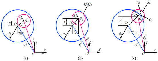
Figure 1.
Kinematic states of revolute clearance: (a) freedom; (b) continual contact; (c) collision.
The coordinates of the centers O1 and O2 of the rotating bearing and shaft in the revolute joint can be represented as:
where the coordinates of member k in the global and local coordinate systems are and , respectively, and is a rotational matrix, which is expressed as:
Eccentricity between the bearing and shaft is denoted as:
The unit vectors of the excenter vectors for bearings and shafts are as follows:
where denotes the magnitude of the excenter vector.
If there is a collision between the hole in bearing and shaft, relative collision depth is expressed as:
where represents the clearance size of the revolute joint, which is the dimensional error between the bearing and the shaft, and can be expressed as:
Therefore, the criterion for determining collisions among the components within a revolute joint with clearance is:
The precise moment of collision between and is determined by the following equation:
In a system of fixed coordinates, the location of the collision point vector can be represented as:
The velocity vector at point of collision when bearing and shaft collide with each other is:
where represents the first derivative of eccentric vector with unit vector .
The collision point on bearing has velocity components in the normal and tangent directions with respect to the axes, and these are described as:
where rotate vector ninety degrees counterclockwise to get tangential vector .
2.2.1. Collision Force Modeling in the Normal Direction
Due to the presence of clearance in kinematic pairs, the kinematic constraints between the components at the kinematic pairs transform into force constraints. Modeling of the collision forces at the clearances is the basis for study of kinetic properties of the mechanism with clearances. This paper primarily focuses on an in-depth study of the L-N model, which is further optimized and improved upon the basis of the Hertz model, thereby providing more precise theoretical support at the academic level for dynamic analysis of machines with clearances.
The Hertz model equation is expressed as:
A more comprehensive consideration of energy losses in the L-N model, represented by the normal force, is represented by:
where represents the normal impact force, represents the impact depth, n is the correction coefficient, K denotes the impact stiffness, D denotes the damping factor, and represents speed of penetration depth.
In Equation (12), the expression for K is given by:
where , and represent the Poisson’s ratios of materials, and and denote their elastic moduli.
The expression for D is given by:
where represents the recovery factor and indicates the original shock speed at the collision point.
2.2.2. Constructing a Model for Tangential Friction
The Coulomb model is a commonly selected force model for considering friction in revolute joints. Friction in this model is proportional to the applied pressure, and its opposite of the direction of the sliding speed relative to it. This study adopts the modified Coulomb friction model proposed by Ambrosio, which introduces a dynamic correction factor to solve the problem of numerical integration instability caused by friction directions close to zero velocity [44]. This correction method can effectively smooth the transition process of friction force and avoid the numerical divergence phenomenon when the velocity crosses zero. This law has been used in many studies [45,46,47].
The corrected model of Coulomb friction is denoted as [44]:
where represents the normal impact force, denotes the friction coefficient, and is the correction factor for dynamics, whose expression is given by:
where represents relatively sliding speed and and denote the speed thresholds for static friction and kinetic friction, respectively.
Force and moment which is operating on center point of bearing can be expressed as:
where and represent the contact components acting in X and Y bearing directions, respectively, and denotes moment acting on centroid of the bearing.
Force and moment acted on the center point of shaft can be shown as:
where and represent the contact components acting in X and Y axial directions, respectively, and denotes torque acting on the centroid of the axis.
2.3. Establishment of a Kinematic Model for the Clearance in Prismatic Joints
The clearance model for prismatic joints, as illustrated in Figure 2. The length, width, and thickness of the slider are denoted as L, , and T, respectively, while the distance between the two sides of the guideway is . The variable a represents half perimeter of rectangular contact surface of slider, and is given by . The clearance value for the prismatic joint is denoted as , and its expression is as follows:
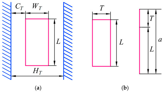
Figure 2.
Clearance model of prismatic joint: (a) main view; (b) side view.
Positional relationship between the slider and guideway is illustrated in Figure 3.
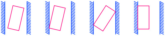
Figure 3.
Positional relationship between slider and guideway.
The analytical model for the clearance in prismatic joints is illustrated in Figure 4. The slider is denoted as component m, and the guideway as component n. and represent the centroids of the slider and guideway, respectively. and denote the local coordinate system of the slider and the guideway respectively. The system coordinate system is represented by O-XY.
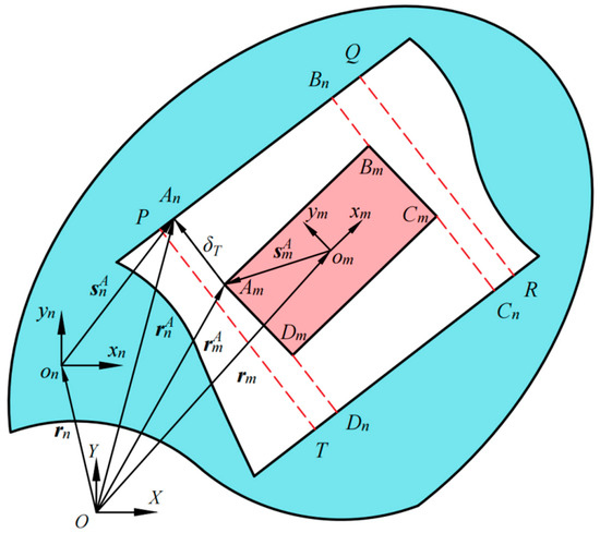
Figure 4.
Analysis model for clearance in prismatic joint.
Suppose that P, Q, R, and T are geometrically constrained points on rail that may come into contact with slider and suppose that , and represent four corners of the slider. Similarly, , and denote points on the guideway that are closest to the corners of the slider. Due to the similarity in the positional equations for each corner point on the slider, take point A as an illustration. The vector of positions of any point H on the i-component can be shown as:
where represents the position vector of centroid of component i in fixed coordinate system, is matrix of transformations, and indicates the vector of positions of any point H in local coordinate system.
Position vector connecting point on the slider and point on the guideway is:
The normal vector on the surface of the guide rail is:
where and are components of the tangential vector in X and Y directions, respectively.
When a collision occurs between slider and guide rail, vector and normal vector of the guideway surface are collinear and oriented in opposing direction.
Consequently, the collisions of the slider with the rail are conditional on [44].
The embedment depth of guide and slider is:
2.3.1. Establishment of Normal Impact Force Model
When corners of two adjacent sliders contact with guide rail, the impact force generated between sliders and the guide rail acts on center of mass of embedded area, as shown in Figure 5a.
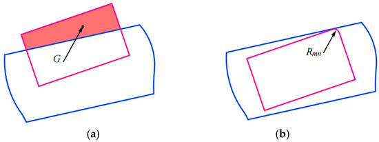
Figure 5.
Contact modes between slider and guide rail: (a) impact occurs through surface contact; (b) impact occurs through contact between a plane and a spherical surface.
Impact force is represented as:
where the factor of stiffness K can be represented as [44]:
where a denotes half perimeter of the slide’s rectangular contact surface, , as illustrated in Figure 2, and , the symbols and indicate Poisson’s ratios of the material, and and represent elastic moduli.
As shown in Figure 5b, when one or both of the opposing slider corners come into contact with the guide rail surface, assuming the contact occurs between a spherical surface and a plane, the contact force model can be represented as [44]:
where the stiffness coefficient K can be formulated as:
Damping factor D is represented as:
where represents the radius of the curvature of the slider’s rotational angle.
2.3.2. Establishment of a Tangential Friction Model
The friction force within the clearance of prismatic joints can be modeled using the friction model investigated in Section 2.2.2.
The forces and torque on centroid of slider can be represented as:
where represents the active force on centroid of slider and represents the torque on the centroid of slider.
3. Establishment of Rigid Body Dynamics Model for Mechanisms with Clearances
3.1. Structural Characteristics of an Eight-Bar Mechanism
The schematic structure of planar eight-bar mechanism is illustrated in Figure 6. The red dotted line indicates the objects at the same vertical position in the Y-axis direction. Mechanism including a crank 1 (L1), triplex member 3 (), connecting rods 2 (L2), 4 (L4), 5 (L5), and 6 (L6), a slider 7, and a frame 8. Crank 1 is the active member, and the slider undergoes reciprocal linear motion within a guideway.
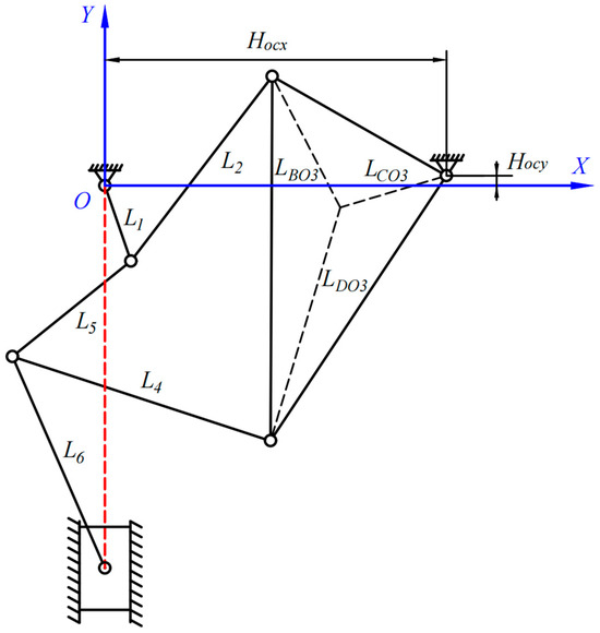
Figure 6.
Simplified structural diagram of a planar eight-bar mechanism.
This study investigates an eight-bar mechanism that has excellent kinematic characteristics, including low-speed stability of the slider in the lower dead center position, pronounced fast slewing characteristics, and strong load carrying capacity. The study focuses on the eight-bar mechanism, which has excellent kinematic characteristics. At the same time, output motion pattern of the eight-bar press can be easily adjusted by controlling and regulating the servomotor without changing the topology of the mechanism. This adjustment improves the stroke, speed, and acceleration volatility of the press slide during the working stroke. As a result, the vibration and shock loads generated during press operation are reduced, thereby improving the operating efficiency of the press.
The design of the eight-bar mechanism is adapted to the needs of diversified products and material processing technologies and has a wide range of potential applications in different industrial fields, for example, machining, automotive manufacturing, and aerospace. High-performance output realized through the intelligent control method not only enhances the adaptability and flexibility of the equipment, but also provides scientific basis and technical support for improving the precision and efficiency of the industrial production process. Therefore, it is of great value for both academic research and engineering applications.
As illustrated in Figure 6, for a planar eight-bar mechanism, the formula for calculating its degree of freedom is:
In the equation, F represents the degree of freedom of mechanism, n denotes the total number of moving links in mechanism, is the number of lower pairs, and is the number of higher pairs.
In this particular mechanism, ; therefore, the degree of freedom F is 1. The mechanism is driven by a single motor. Consequently, this mechanism possesses a definite motion.
3.2. Establishment of a Rigid Body Dynamics Model with Mixed Clearances
Rigid body dynamics analysis diagram of the eight-bar mechanism. In Figure 7, global coordinate system origin is set to point O, while origins of local coordinate systems are typically set at centroid of each component. Global coordinates of for each component are indicated as:
where and represent coordinates of the centroid of component i in global coordinate system, respectively, while denotes angle of component i relative to x-axis in the global coordinate system.
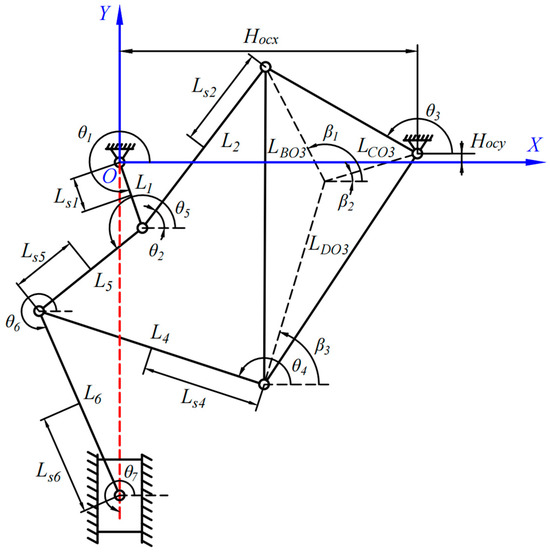
Figure 7.
Schematic diagram of coordinates for a planar eight-bar mechanism.
The velocities and accelerations of the components of each global coordinate system are expressed as follows, respectively:
Generalized coordinates of an eight-bar mechanism system are represented as:
In the equation, there are a total of 21 generalized coordinates. The generalized velocities of system is and generalized accelerations of system is .
When considering mixed clearances (composite revolute clearance A and prismatic clearance F), crank 1 and connecting rod 2 are joined by a rotating pair , crank 1 and connecting rod 5 are joined by a rotating pair , forming the composite revolute joint A. Slider and guide rail constitute prismatic joint F. Whenever a clearance exists, the constraint equations of the system will be reduced by two, meaning that the displacement constraints in both horizontal and vertical directions of the ideal planar kinematic pairs are released. At this point, the mechanism has a total of seven revolute joint constraints. Compared to constraint equations of ideal mechanism, the constraint equations of eight-bar mechanism with mixed clearances (composite revolute clearance A and prismatic clearance F) are reduced by six. The initial driving angles have been obtained through the inverse kinematics solution during the simulation process, and the system has a total of 15 constraint equations.
Since crank 1 is directly driven by a motor, the prismatic joint clearance is directly related to the slider. Therefore, investigating the clearances at the composite revolute joint A and the prismatic joint F can effectively reflect the influence of mixed clearances on the dynamics of the mechanism.
Figure 8 illustrates structure of an eight-bar mechanism with mixed clearances (composite rotation clearance A and prismatic clearance F).
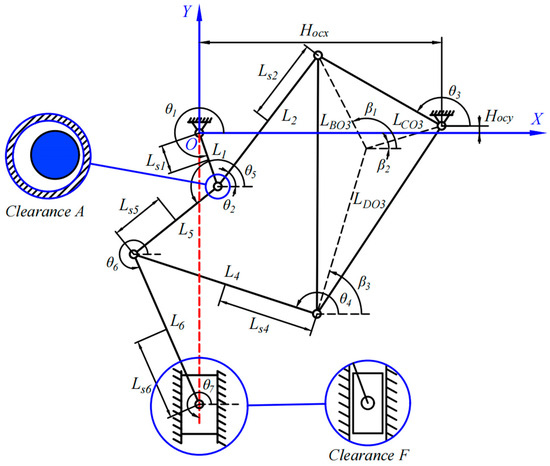
Figure 8.
Structural diagram of an eight-bar planar mechanism with mixed clearances.
Each feature frame can be connected to feature frames on adjacent parts, and there are some mathematical constraints between adjacent frames. To ensure the position and orientation of a part with respect to its neighbors, it is necessary to impose the corresponding mechanical constraints between parts as well as assembly features [48]. The displacement constraint equation of mechanism when mechanism has a mixed clearances can be expressed as:
where 4.2649 represents the radian value of the initial direction angle obtained when crank 1 rotates counterclockwise from the x-axis.
By taking the first-order derivative with respect to time of Equation (39), the velocity constraint equation of the system can be obtained as follows:
where represents Jacobian matrix, and represents derivate of bound equation with respect to time, .
Jacobian matrix of an institution can be represented as:
When a rigid body mechanism has mixed clearances, the time partial derivative of the constraining equation is written as:
Differentiating Equation (40) by time yields the equation of acceleration constraints:
where , .
Establish system dynamics equations based on the Lagrange multiplication:
where the matrix M represents mass matrix, is a column vector of Lagrange multipliers, which accounts for internal forces and moments between components connected by revolute joints, and g denotes column vector of generalized external forces.
Quality matrix of the system is written as:
From Equations (43) and (44), system dynamics equations are expressed as follows:
From Equation (46), it can solve for the two variables and . However, Equation (46) involves no displacement and velocity constraints, which can lead to constraint violations and computational divergence when solving the equation. Based on this phenomenon, an algorithm for constraint stabilization was introduced by Baumgarte that acceleration constraint equation contains both displacement and velocity constraints in order to enhance the stability of the solution. The resulting new dynamic equation is as follows:
where and are correction parameters greater than 0, .
4. Dynamic Precision Reliability Modeling of Multilink Mechanisms with Clearances
4.1. The Theory of Stress–Strength Interference
In the field of mechanical equipment, once key components fail, it is highly likely to cause the entire equipment to malfunction. The reason why parts fail is often because the load they bear during actual operation exceeds the ultimate bearing capacity of the part at the corresponding time. Specifically, during the operation of the component, if its strength value is higher than the stress value it is subjected to, the component can operate normally; on the contrary, when the stress value exceeds the strength value, the part will fail. In addition, due to the randomness of various factors affecting stress and strength, both stress and strength exhibit dispersion characteristics. The relationship between stress and strength can be referred to in Figure 9. From the figure, it can be observed that when the mean value of strength is greater than the mean value of stress, situations where the strength is less than the stress may occur within the “interference zone”.
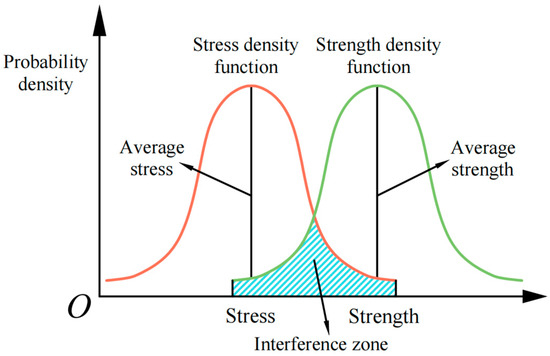
Figure 9.
Model of stress–strength interference.
In accordance with the theory of stress–strength interference, reliability is the probability of strength exceeding stress, which is denoted as:
where S denotes strength, s represents stress, and indicates the safety margin. When , the mechanical system operates normally. Assuming that both stress and strength are normally distributed, and leveraging property that sum (or difference) of normally distributed variables is also normally distributed, safety margin Z likewise follows a normal distribution.
where and represent mean and mean square deviation of strength, respectively, , represent mean and mean square deviation of stress, respectively, and , .
The reliability is the probability that the safety factor , can be represented as:
Transform Equation (50) into the standard normal distribution form
where , , .
Define the reliability indicator as
From Equations (51) and (52), the reliability is calculated as
The above equation represents the formula for calculating the structural reliability when there are strengths and stresses obeying a normal distribution.
4.2. Mechanism Dynamically Precise Reliability Model
Assuming that operation time of mechanism is denoted as , the function of error is defined as:
where represents the slider’s actual position and denotes the slider’s ideal position. The error limit is defined as , when the mechanism is reliable and vice versa mechanism fails.
Based on theory of stress–strength interference, reliability of mechanism under various clearance conditions is addressed by assuming that both the actual errors and permissible error of the slider follow normal distributions. Real error of the slider serves as the stress, while the permissible error of the slider represents the strength.
Using the theory of stress–strength interference as a foundation, and taking calculation of displacement reliability as an example, within a time range for the mechanism, the reliability index for displacement can be obtained.
where and represent mean and RMS of allowable displacement error, respectively, and and denote mean and mean square deviation of displacement errors, respectively.
Reliability of mechanism’s displacement is denoted as:
A rigid body dynamics model of a multilink mechanism can be established to solve for and . Instead, the mean and RMS deviation of the permissible displacement tolerances is calculated by the following formulae:
where and denote the maximum and minimum bounds of allowable tolerance, respectively.
5. Response Analysis of Rigid Body Dynamics of Clearance Containing Mechanism
5.1. Simulation Parameters for an Eight-Bar Mechanism with Clearance
This section defines the simulation parameters of an eight-bar mechanism, which are crucial for modeling its dynamic behavior under clearance effects. The parameters are divided into three tables: components’ masses and moments of inertia (Table 2), lengths of various components (Table 3), and kinematic clearance specific parameters (Table 4). The values in Table 2, Table 3 and Table 4 are derived from the SolidWorks2021 model of the institution.
Table 2.
Components’ masses and moments of inertia.
Table 3.
Lengths of various components.
Table 4.
Kinematic clearance-specific parameters.
5.2. Impact of Different Clearance Types on the Rigid Body Dynamic Response in a Mechanism
In the current section, the impact of varying clearance types on kinematic characteristics of mechanism is examined, specifically: compound external rotation joint clearance, prismatic joint clearance, and mixed clearances. The values for all clearances are configured as 0.2 mm, while the driving speed of crank 1 is set to 60 rpm. Figure 10 illustrates curves depicting impact of various clearance types on the motion characteristics of the slider.
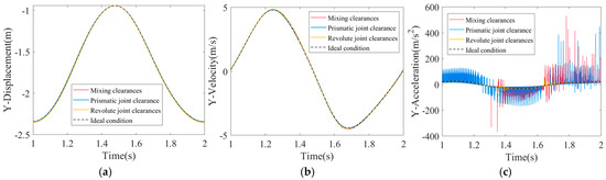
Figure 10.
Kinematic characteristics of the slider under different types of clearance: (a) slider displacement; (b) slider velocity; (c) slider acceleration.
The results presented in Figure 10 indicate that various types of clearances have a relatively minor effect on displacement response curves, with displacement curves closely aligning with the ideal curve and exhibiting good smoothness. Compared to the acceleration response curve of the slider, the velocity response curve exhibits slight fluctuations around the ideal curve, while the acceleration response curve demonstrates more significant fluctuations and peak phenomena. Analysis reveals that mixed clearances have the most prominent effect on acceleration characteristics of slider, followed by prismatic joint clearance, and comparatively, the revolute joint clearance has the smallest impact. Specifically, when the mechanism only contains revolute joint clearance, only contains prismatic joint clearance, and contains mixed clearances, the maximum acceleration deviations reach 51.4 m/s2, 448.3 m/s2, and 531.2 m/s2, respectively.
5.3. Effect of Combined Clearances on Rigid Body Dynamic Response of Mechanism
This section analyzes the impact of mixed clearances on the rigid body dynamic response of the mechanism. The L-N model and modified Coulomb friction models are used for normal impact and tangential friction, respectively, in the study of influence of various clearance values and travelling speeds on dynamic response of rigid body of an eight-bar mechanism.
5.3.1. Effect of Clearance Values in the Response of Rigid Body Dynamics of Mixed Clearance Mechanism
In this section, influence of clearance values on dynamic response of mechanism in presence of a mixed clearances will be investigated, with particular reference to the effect of 0.1 mm, 0.2 mm, and 0.3 mm clearance values. Assuming that clearance values of composite external joint clearance A and prismatic joint clearance F are the same. Figure 11 and Figure 12 illustrate at drive speed of crank 1 set to 60 revolutions per minute, the dynamic response of mechanism with a clearance friction coefficient of 0.2.
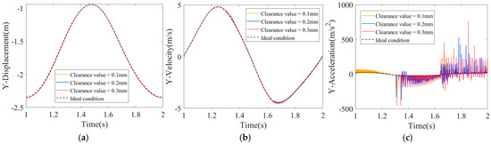
Figure 11.
Motion characteristics of slider with various clearance values: (a) slider displacement; (b) slider velocity; (c) slider acceleration.
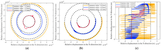
Figure 12.
Center trajectories at clearances with different values: (a) revolute joint clearance A1; (b) revolute joint clearance A2; (c) prismatic joint clearance F.
Figure 11 shows displacement, velocity, and acceleration graphs of the slider under mixed clearances (combined external rotary clearance A and prismatic clearance F) with clearance values of 0.1 mm, 0.2 mm, and 0.3 mm, respectively. The kinematic characteristics show that characteristics of displacement and velocity of a slider mixed clearances mechanism with different values of the clearances show a relatively stable trend, with the displacement curves close to the ideal state, while the velocity curves have a slight fluctuation. As the clearance value gradually increases, peak acceleration is delayed, and its value shows an obvious upward trend. Specifically, the peak acceleration of the slider occurs at 1.67 s with a value of 305.1 m/s2 at 0.1 mm, at 1.78 s with a value of 531.2 m/s2 at 0.2 mm, and at 1.85 s with a value of 766.5 m/s2 at 0.3 mm. Wear-induced clearances will lead to an increase in motion pair clearances, thereby increasing relative motion space between components of mechanism. Larger clearances allow for greater ranges of motion, directly resulting in an increase in the maximum values of slider displacement, velocity, and acceleration.
As shown in Figure 12, the center trajectories at the clearances of revolute joint , revolute joint , and prismatic joint F reveal that, with clearance values of 0.1 mm, 0.2 mm, and 0.3 mm, respectively, as the clearance value of the kinematic pair increases, the center trajectories at clearances exhibit increasingly complex dynamic characteristics. These are manifested as increased frequencies of free motion states and collision events of the shaft within the bearing and slider on the guideway. This variation leads to deviations in dynamic behavior between the actual mechanism with clearances and theoretically ideal mechanism. As clearance size increases from 0.1 mm to 0.3 mm, eccentricity between shaft and bearing and between slide and the guideway increases accordingly due to a significant increase in clearance width. This change in geometry leads to a significant increase in instantaneous collision forces in the clearance region, which deepens the depth of penetration of the shaft into the bearing and the slide into the guideway. Together, these effects influence dynamic response of mechanism in terms of faster vibration frequency and higher vibration amplitude, which further affects the kinematic and dynamic behavior of the mechanism at a deeper level.
5.3.2. Effect of Driving Speed on Dynamic Response of the Rigid Body of a Mixed Clearance Mechanism
In order to investigate the effect of driving speed on the rigid-body dynamic response of a mechanism containing a mixed clearance (a combination of external rotary joint clearance A and prismatic joint clearance F), three sets of speeds were chosen for the study, i.e., 30 rpm, 60 rpm, and 150 rpm for crank 1. The clearance values were set to 0.2 mm. The displacement, velocity, and acceleration plots of the slider as well as the center trajectories for different clearances are shown in Figure 13, Figure 14, Figure 15 and Figure 16.
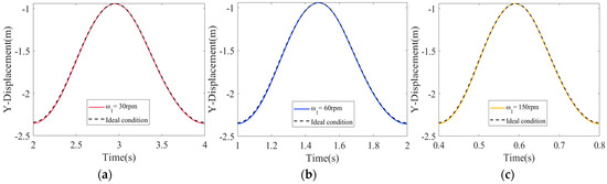
Figure 13.
Displacement of the slider: (a) ω1 = 30 rpm; (b) ω1 = 60 rpm; (c) ω1 = 150 rpm.
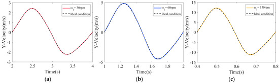
Figure 14.
Velocity of the slider: (a) ω1 = 30 rpm; (b) ω1 = 60 rpm; (c) ω1 = 150 rpm.
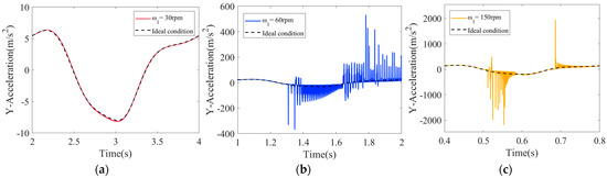
Figure 15.
Acceleration of the slider: (a) ω1 = 30 rpm; (b) ω1 = 60 rpm; (c) ω1 = 150 rpm.
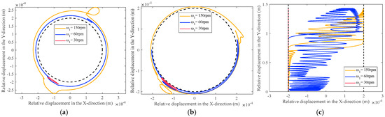
Figure 16.
Center trajectories at clearances with different driving speeds over time: (a) revolute joint clearance A1; (b) revolute joint clearance A2; (c) prismatic joint clearance F.
As illustrated in Figure 13, Figure 14 and Figure 15, as the driving speed of crank 1 increases from 30 rpm to 60 rpm, and then to 150 rpm, the peak values and vibration frequencies of the dynamic responses also increase accordingly. The driving speed has a direct impact on the relative motion states between components in clearance kinematic pairs, accelerating the transition rates of motion states between the shaft and the bearing, and subsequently, intensifying the wear process of the kinematic pairs. The displacement, velocity, and acceleration graphs of the slider show that, in mechanisms with mixed clearances, peak displacement of slider exhibits high stability and is almost unaffected by the presence of clearances. Furthermore, as driving speed gradually increases, velocity fluctuations of slider significantly intensify, with peak velocity also increasing. An intensification of acceleration fluctuations of the slider similarly results from an increase in driving speed, and the peak acceleration values also increase notably. Specifically, when driving velocity is 30 rpm, the maximum acceleration value is 8.2 m/s2. When driving velocity is 60 rpm, the maximum acceleration value reaches 531.2 m/s2. When driving velocity is 150 rpm, the maximum acceleration value soars to 2183.5 m/s2. In some data plots, there are instantaneous changes in values at several positions. For instance, in the acceleration data plot Figure 15b, during the time interval from 1.3 s to 2 s, there are two significant fluctuations, mainly concentrated in two regions. These fluctuations are primarily caused by the collisions between the slider and the guide rail. This indicates that during this stage, the four collision states transition relatively frequently, resulting in high-incidence collision zones. Especially when the clearance is small, the mechanism is more prone to being in a state of continuous contact and collision, thereby leading to an increase in the oscillation frequency and abrupt changes in the values of velocity and acceleration.
This is illustrated in Figure 16, where center trajectories for the second cycle are analyzed. When the drive speed is increased from 30 rpm to 150 rpm, collision frequency between the shaft and the bearing is accelerated, leading to a more confused and disorganized state of movement of the shaft and slider in the bearing on the guideway. This leads to an increase in collision forces between components, exacerbating the degree of confusion in the center trajectory at the clearance and making recoil and prismatic joints more prone to failure. As the drive velocity rises, the center trajectory becomes more chaotic and freer and collision states occur more frequently. As the mechanism operates at higher speeds, the relative speed of motion between the shaft and bearings increases. Due to the presence of clearance or friction, the motion of the shaft inside the bearing may become unstable, leading to sudden changes in acceleration. As can be seen from the acceleration and center trajectory, large fluctuations can occur within a cycle, which are mainly due to collisions between shaft and bearing, which are focused on two specific areas of impact.
6. Nonlinear Characterizations of Rigid Multilink Mechanism with Clearances
In this section, the influence of various clearance values and driving velocities on the nonlinear characteristics of a stiff multilink structure with mixed clearances, phase plane analysis, and Poincaré plot analysis are used for the discussion, respectively. Clearance value and drive speed are essential to influence the mechanism’s nonlinear characteristics. Phase plane analysis method is a direct observation technique that allows a geometrical representation of the reciprocal acyclic kinematic properties of chaotic motions in terms of phase plane maps. The Poincaré map analysis method provides an effective method to studying chaotic motion, which enables a more precise determination of the chaotic phenomena at the clearance.
6.1. Effect of Clearance Values on Nonlinearity Characteristics of Rigourous Multilink Structures with Mixed Clearances
Assuming equal clearance values at the composite revolute pair clearance A (consisting of rotating pair clearance and rotating pair clearance ) and the prismatic pair clearance F, a comparative analysis is conducted to investigate the effect of clearance values of 0.1 mm, 0.2 mm, and 0.3 mm on the motion states of the revolute pairs and sliders with mixed clearances. The driving speed of crank 1 is uniformly set at 60 rpm. Phase portraits and Poincaré maps for rotating pair clearance , rotating pair clearance , and prismatic pair clearance F are illustrated in Figure 17, Figure 18, Figure 19 and Figure 20.
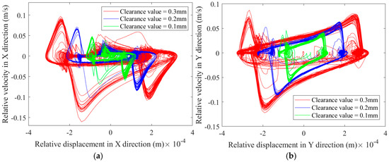
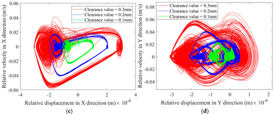
Figure 17.
Phase diagram at the joint clearance of revolute pair: (a) phase diagram of clearance A1 in the X-direction; (b) phase diagram of clearance A1 in the Y-direction; (c) phase diagram of clearance A2 in the X-direction; (d) phase diagram of clearance A2 in the Y-direction.
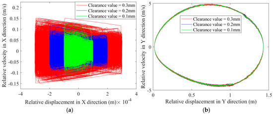
Figure 18.
Phase diagram at the clearance of prismatic joint: (a) phase diagram of clearance F in the X-direction; (b) phase diagram of clearance F in the Y-direction.
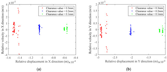
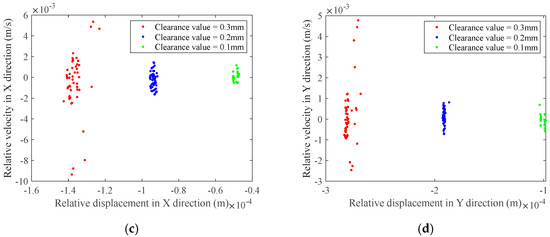
Figure 19.
Poincaré map at the clearance of revolute pair: (a) Poincaré map of clearance A1 in the X-direction; (b) Poincaré map of clearance A1 in the Y-direction; (c) Poincaré map of clearance A2 in the X-direction; (d) Poincaré map of clearance A2 in the Y-direction.
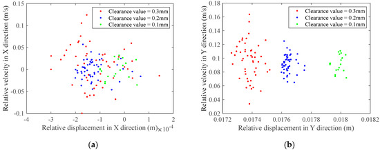
Figure 20.
Poincaré map at the clearance of prismatic joint: (a) Poincaré map of clearance F in the X-direction; (b) Poincaré map of clearance F in the Y-direction.
As shown in Figure 17, Figure 18, Figure 19 and Figure 20, phase portraits and Poincaré maps at rotating pair clearance , rotating pair clearance , and prismatic pair clearance F reveal that with the rise in clearance values, the scope of the phase portraits and the Poincaré maps expands, the scattering degree of the mapped points rises, resulting in a more pronounced chaotic phenomenon. Under different clearance values, the phase trajectories in the X and Y direction phase diagrams of revolute pair , revolute pair , and prismatic pair F, spanning horizontal and vertical regions, are presented in Table 5.
Table 5.
The phase portrait range of rotation pair A1, rotation pair A2 and prismatic pair F under different clearance values.
From the data shown in Figure 17 and Figure 18 and Table 5, it is evident that, as the clearance size rises, the degree of disorder in the phase diagrams at revolute clearance , revolute clearance , and prismatic clearance F intensifies, accompanied by an expansion of the chaotic regions. This chaos originates from intermittent collisions and nonlinear contact forces caused by clearances, leading to instability and energy dissipation of the motion trajectory, indicating a decrease in motion accuracy. The expansion of the phase diagram range is related to higher energy dissipation and chaotic effects between joint surfaces. In the Poincaré maps at revolute clearance and revolute clearance , as illustrated in Figure 19, it can be seen that as the clearance value increases, a range of mapped points at revolute clearance and revolute clearance expands, indicating enhanced chaotic behavior and increasingly severe damage to the revolute joints with clearances. The Poincaré mapping transforms from clustered points to dispersed points, confirming the bifurcation into chaos at larger clearances. The Poincaré plots of the prism clearance F in Figure 20 shows that the proportion of area occupied by the mapped points increases as the clearance value increases, and all the points are approximately circular in shape. Although the phase diagram of the moving pair F shows a large range in the Y direction, its Poincaré mapping points are approximately circularly distributed; it can be inferred that the slider exhibits a periodic motion without confusion.
6.2. Driving Speed Effect on Mixed Clearance Rigid Multilink Mechanism Nonlinear Characteristics
Assuming that clearance values of the rigid multilink mechanism with mixed backlash are all 0.2 mm, drive speed of crank 1 is chosen to be 30 rpm, 60 rpm, and 150 rpm to investigate the impact of driving speed on nonlinear characteristics of multilink mechanism. Figure 21 and Figure 22 show phase diagrams of rotating joint and rotating joint in the X and Y directions, respectively, and the phase diagram of prismatic joint F. Figure 23 and Figure 24 show the Poincaré plots of rotating joint and rotating joint in the X and Y directions, respectively, and Poincaré plots of prismatic joint F.
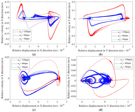
Figure 21.
Phase diagram at the joint clearance of revolute pair: (a) phase diagram of clearance A1 in the X-direction; (b) phase diagram of clearance A1 in the Y-direction; (c) phase diagram of clearance A2 in the X-direction; (d) phase diagram of clearance A2 in the Y-direction.
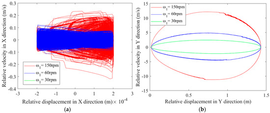
Figure 22.
Phase diagram at the clearance of prismatic joint: (a) phase diagram of clearance F in the X-direction; (b) phase diagram of clearance F in the Y-direction.
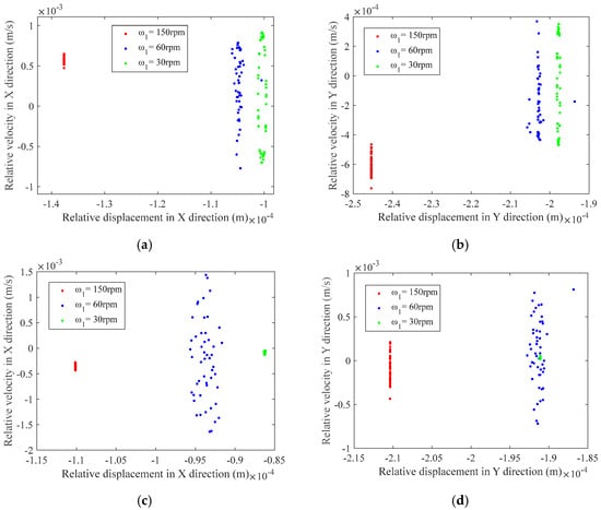
Figure 23.
Poincaré map at the clearance of revolute pair: (a) Poincaré map of clearance A1 in the X-direction; (b) Poincaré map of clearance A1 in the Y-direction; (c) Poincaré map of clearance A2 in the X-direction; (d) Poincaré map of clearance A2 in the Y-direction.
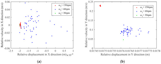
Figure 24.
Poincaré map at the clearance of prismatic joint: (a) Poincaré map of clearance F in the X-direction; (b) Poincaré map of clearance F in the Y-direction.
Based on Figure 21 and Figure 22, it is inferred that driving speed has a material impact on multilink mechanism nonlinear characteristics with mixed clearance. With increasing drive speed of crank 1, the area of the phase portrait increases. The phase trajectories of rotation pair , rotation pair , and prismatic pair F across horizontal and vertical regions in the X and Y direction phase diagrams at different driving speeds are shown in Table 6.
Table 6.
The phase range of rotation pair A1, rotation pair A2, and prismatic joint F varies at different driving speeds.
From Figure 21, which depicts the phase portraits at revolute joints and , it is seen that as the drive velocity rise from 30 rpm to 60 rpm and further to 150 rpm, the degree of chaos increases, and the chaotic regions expand accordingly. The impact caused by rebound becomes more frequent and intense, and the expanding phase space region means it is becoming increasingly unpredictable, where small disturbances can cause trajectory divergence. Figure 23, showing the Poincaré maps of revolute joints and , reveals that with continuous rise in driving speed, a range of mapped points at these revolute joints expands, indicating an intensification of chaotic phenomena. Based on the observations from these two figures, it is concluded that damage at the revolute joints becomes increasingly severe. Higher speeds inject kinetic energy, causing components to bounce unpredictably in the clearance area. This will excite higher-order vibration modes, leading to complex non periodic motion. Figure 22 presents the phase portrait at prismatic joint F, which indicates that as driving speed increases, a proportion of mapped points in both X and Y directions expands, with a phase portrait in Y direction resembling a circular ring. The Poincaré map at prismatic joint F, shown in Figure 24, demonstrates that the mapped points in the Y direction are relatively concentrated, with many overlapping, especially at driving speeds of 30 rpm and 150 rpm, where the Poincaré maps are solid small circles. Combined with the trajectory of the prismatic joint’s center, it can be inferred that slider undergoes periodic motion as driving speed continuously increases, without an occurrence of chaotic phenomena.
6.3. The Influence of the Prismatic Joint Clearance on the Nonlinear Characteristics at the Revolute Joint Clearance
Assuming that the clearance values of the rigid multilink mechanism with clearance are all 0.2 mm, and the driving speeds of crank 1 are selected as 60 rpm, the influence of the clearance of the moving pair on the nonlinear characteristics at the clearance of the compound rotating pair of the multilink mechanism is studied. Figure 25 shows the phase diagrams of revolute joint and revolute joint in the X and Y directions. Figure 26 shows the Poincaré maps of revolute joint and revolute joint in the X and Y directions.
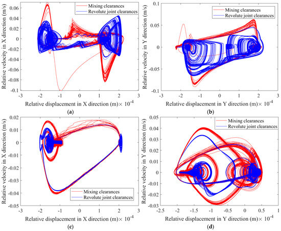
Figure 25.
Phase diagram at the joint clearance of revolute pair: (a) phase diagram of clearance A1 in the X-direction; (b) phase diagram of clearance A1 in the Y-direction; (c) phase diagram of clearance A2 in the X-direction; (d) phase diagram of clearance A2 in the Y-direction.
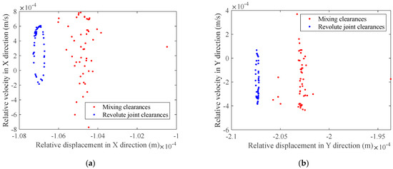
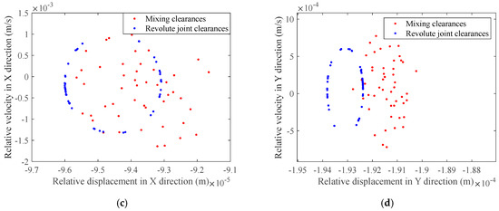
Figure 26.
Poincaré map at the clearance of revolute pair: (a) Poincaré map of clearance A1 in the X-direction; (b) Poincaré map of clearance A1 in the Y-direction; (c) Poincaré map of clearance A2 in the X-direction; (d) Poincaré map of clearance A2 in the Y-direction.
As can be seen from Figure 25, the phase diagram region with mixed clearances at the revolute joint clearances exceeds that with compound revolute joint clearances, indicating a higher degree of chaos and a more pronounced tendency of expansion. The corresponding Poincaré maps in Figure 26 show that the Poincaré mapping points at the revolute joint clearances under mixed clearances are more divergent and disordered. In contrast, the Poincaré mapping points at the revolute joint clearances under compound revolute joint clearances are more concentrated, have a higher degree of repetition, and are relatively more concentrated and ordered. From this, it can be inferred that the introduction of the prismatic joint clearance F makes the nonlinear characteristics at the revolute joint clearances more pronounced, with greater chaotic properties, and the motion accuracy of the mechanism is affected.
7. Dynamic Precision Reliable Analysis of Multilink Structure with Clearance
7.1. Influence of Clearance Values on Reliable Dynamic Accuracy of Hybrid Clearance Mechanisms
This subsection investigates impact of clearance values on dynamic precision reliability of mechanisms with clearances. Friction coefficient at clearance is set to 0.2, driving speed is uniformly 60 rpm. Clearance values are taken as 0.1 mm, 0.2 mm, and 0.3 mm, respectively. Displacement and velocity curves do not change much due to the effect of the clearance, so the selection phenomenon is more intuitively accelerated. The reliability indices and reliability of slider acceleration are illustrated in Figure 27.
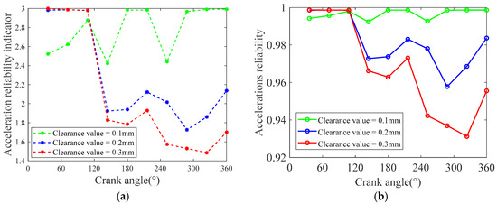
Figure 27.
(a) Reliability indices of slider acceleration; (b) reliability of slider acceleration.
As illustrated in the Figure 27, clearance values are 0.1 mm, 0.2 mm, and 0.3 mm, respectively, and the corresponding reliability indices of the minimum acceleration of the slider are 2.4244, 1.7258, and 1.4850. The figures also indicate that the reliabilities of the minimum acceleration of slider corresponding to different clearance values are 0.9923, 0.9578, and 0.9312, respectively. This trend arises from the amplification of kinematic uncertainty at larger clearances. Increased clearance allows for greater free motion between joints, leading to impulsive forces during contact transitions. These forces induce higher-frequency vibrations and transient accelerations, which degrade the repeatability of the slider’s motion. Therefore, for multilink mechanisms with mixed clearances, higher values of clearance result in lower reliability of the dynamic accuracy of the slider. A reliability of 0.93 implies a 7% probability that the slider’s acceleration will fall below the required minimum during operation. This level is sufficient to meet the requirements for mechanism accuracy and reliability in most industrial production. However, in high-precision industrial applications such as aerospace, there is a high demand for mechanism accuracy, and further improvement and optimization of mechanism design and motion are still needed. Design changes—such as reducing clearance tolerances or implementing active damping—should be considered when reliability falls below application-specific safety margins.
7.2. Influence of Travelling Speed on Reliability of the Dynamic Accuracy of a Mixed Clearance Mechanism
This subsection investigates impact of various drive speeds on dynamic accuracy reliability of multilink mechanisms with mixed clearances. Assuming that clearance values are all 0.2 mm, the driving speeds are set to 30 rpm, 60 rpm, and 150 rpm, respectively. The reliability indices and reliabilities of the slider acceleration are shown in Figure 28.
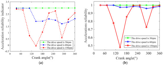
Figure 28.
(a) Reliability indices of slider acceleration; (b) reliability of slider acceleration.
As illustrated in the Figure 28, when driving speeds are 30 rpm, 60 rpm, and 150 rpm, respectively, the corresponding reliability indices of the minimum acceleration of the slider are 2.9985, 1.7258, and −0.0569. The figures also indicate that the reliabilities of the minimum acceleration of slider corresponding to various driving velocities are 0.9986, 0.9578, and 0.4772, respectively. The sharp decline in reliability at higher speeds is driven by inertial effects and reduced time for dynamic stabilization. At 150 rpm, the mechanism’s inertia dominates over joint damping, causing chaotic contact forces and resonance phenomena. This leads to unpredictable acceleration spikes that exceed the failure threshold, significantly increasing the probability of dynamic failure. Therefore, for multilink mechanisms with mixed clearances, higher drive speeds result in less reliable dynamic accuracy of the slider. The acceleration reliability is 0.47, which deviates significantly from the ideal acceleration envisioned, which makes this mechanism almost unsuitable for industrial tasks that require strict acceleration control. When the reliability is below 0.90, design changes are crucial and can be improved by optimizing the mechanism design, introducing speed related damping, or using adaptive control measures.
8. Conclusions
In this paper, the eight-bar structure of a mixed multilink pressing machine is investigated, and a rigid-body dynamics modeling method for mixed clearances mechanism based on Lagrange multiplier method is proposed. The study examined the dynamic answer of eight-bar mechanisms under various clearance types. A study is conducted on the dynamics of an eight-bar mechanism with mixed clearances, focusing on the influence of clearance sizes, drive speeds, and other factors on the dynamic responses and nonlinear characteristics of the mechanisms, as well as dynamic accuracy reliability of the multilink mechanism.
Research results indicate that the type and size of clearance have a comparatively small effect on displacement and velocity, but a large influence on acceleration. Driving speed significantly affects the central trajectories at various clearance locations. Phase portraits and Poincaré maps, which vary with clearance values and driving speeds, reveal a clear trend in the nonlinear characteristics of the mixed clearance mechanism. Due to the coupling effect of revolute joint clearances and prismatic joint clearances, it is found that when clearance size and driving speed are large, mixed clearances significantly affect nonlinear characteristics of the mechanism. Within the parameter range studied in this chapter, the slider is less affected by parameters and remains in a periodic motion state throughout. Simultaneously, it is concluded from the models of reliability of dynamic accuracy of the mechanism that a smaller clearance size and a smaller drive speed result in a higher dynamic accuracy reliability of mechanisms.
Author Contributions
Conceptualization, Y.L. and S.J.; methodology, Y.L. and S.J.; software, Y.L. and J.Z.; validation, Y.L., J.Z, Q.Z. and M.C.; formal analysis, Y.L. and J.Z.; investigation, J.Z.; resources, Q.Z.; data curation, Y.L. and J.Z.; writing—original draft preparation, Y.L. and M.C.; writing—review and editing, Y.L., J.Z. and S.J.; visualization, Y.L.; supervision, S.J.; project administration, S.J.; funding acquisition, S.J. All authors have read and agreed to the published version of the manuscript.
Funding
This research was funded by [Natural Science Foundation of Shandong Province] grant number [ZR2023QE039] And The APC was funded by [Jiang Shuai]; [Open Project of Key Laboratory of Special Motors and High Voltage Electrical Appliances, Ministry of Education] grant number [KFKT202402] And The APC was funded by [Jiang Shuai].
Institutional Review Board Statement
Not applicable.
Informed Consent Statement
Not applicable.
Data Availability Statement
The data used to support the results of this research are included in this paper.
Conflicts of Interest
The authors declare that they have no conflicts of interest.
References
- Song, Z.D.; Yang, X.J.; Li, B.; Xu, W.F.; Hu, H. Modular dynamic modeling and analysis of planar closed-loop mechanisms with clearance joints and flexible links. Proc. Inst. Mech. Eng. Part C J. Mech. Eng. Sci. 2017, 231, 522–540. [Google Scholar] [CrossRef]
- Korayem, M.H.; Dehkordi, S.F.; Mehrjooee, O. Nonlinear analysis of open-chain flexible manipulator with time-dependent structure. Adv. Space Res. 2022, 69, 1027–1049. [Google Scholar] [CrossRef]
- Mehrjooee, O.; Dehkordi, S.F.; Korayem, M.H. Dynamic modeling and extended bifurcation analysis of flexible-link manipulator. Mech. Based Des. Struct. Mach. 2020, 48, 87–110. [Google Scholar] [CrossRef]
- Chen, X.L.; Jiang, S.; Wang, S.Y.; Deng, Y. Dynamics analysis of planar multi-DOF mechanism with multiple revolute clearances and chaos identification of revolute clearance joints. Multibody Syst. Dyn. 2019, 47, 317–345. [Google Scholar] [CrossRef]
- Gao, Y.; Zhang, F.; Li, Y.Y. Reliability optimization design of a planar multi-body system with two clearance joints based on reliability sensitivity analysis. Proc. Inst. Mech. Eng. Part C J. Mech. Eng. Sci. 2019, 233, 1369–1382. [Google Scholar] [CrossRef]
- Xiang, W.W.K.; Yan, S.Z.; Wu, J.N.; Niu, W.D. Dynamic response and sensitivity analysis for mechanical systems with clearance joints and parameter uncertainties using Chebyshev polynomials method. Mech. Syst. Signal Process. 2020, 138, 106551. [Google Scholar] [CrossRef]
- Hou, Y.L.; Deng, Y.J.; Zeng, D.X. Dynamic modelling and properties analysis of 3RSR parallel mechanism considering spherical joint clearance and wear. J. Cent. South Univ. 2021, 28, 712–727. [Google Scholar] [CrossRef]
- Li, Y.Y.; Chen, G.P.; Sun, D.Y.; Gao, Y.; Wang, K. Dynamic analysis and optimization design of a planar slider-crank mechanism with flexible components and two clearance joints. Mech. Mach. Theory 2016, 99, 37–57. [Google Scholar] [CrossRef]
- Bai, Z.; Liu, T.; Li, J.; Zhao, J. Numerical and experimental study on dynamic characteristics of planar mechanism with mixed clearances. Mech. Based Des. Struct. Mach. 2023, 51, 6142–6165. [Google Scholar] [CrossRef]
- Tan, H.; Hu, Y.; Li, L. A continuous analysis method of planar rigid-body mechanical systems with two revolute clearance joints. Multibody Syst. Dyn. 2017, 40, 347–373. [Google Scholar] [CrossRef]
- Olyaei, A.A.; Ghazavi, M.R. Stabilizing slider-crank mechanism with clearance joints. Mech. Mach. Theory 2012, 53, 17–29. [Google Scholar] [CrossRef]
- Zheng, X.; Li, J.; Wang, Q.; Liao, Q. A methodology for modeling and simulating frictional translational clearance joint in multibody systems including a flexible slider part. Mech. Mach. Theory 2019, 142, 103594. [Google Scholar] [CrossRef]
- Zheng, E.; Wang, T.; Guo, J.; Zhu, Y.; Lin, X.; Wang, Y.; Kang, M. Dynamic modeling and error analysis of planar flexible multilink mechanism with clearance and spindle-bearing structure. Mech. Mach. Theory 2019, 131, 234–260. [Google Scholar] [CrossRef]
- Lu, J.; Jiang, J.; Li, J.; Wen, M. Analysis of dynamic mechanism and global response of vehicle shimmy system with multi-clearance joints. J. Vib. Control 2018, 24, 2312–2326. [Google Scholar] [CrossRef]
- Yu, H.; Zhang, J.; Wang, H. Dynamic performance of over-constrained planar mechanisms with multiple revolute clearance joints. Proc. Inst. Mech. Eng. Part C J. Mech. Eng. Sci. 2018, 232, 3524–3537. [Google Scholar] [CrossRef]
- Farahan, S.B.; Ghazavi, M.R.; Rahmanian, S. Bifurcation in a planar four-bar mechanism with revolute clearance joint. Nonlinear Dyn. 2017, 87, 955–973. [Google Scholar] [CrossRef]
- Hou, Y.; Wang, Y.; Jing, G.; Deng, Y.; Zeng, D.; Qiu, X. Chaos phenomenon and stability analysis of RU-RPR parallel mechanism with clearance and friction. Adv. Mech. Eng. 2018, 10, 1–15. [Google Scholar] [CrossRef]
- Wang, Z.; Tian, Q.; Hu, H.; Flores, P. Nonlinear dynamics and chaotic control of a flexible multibody system with uncertain joint clearance. Nonlinear Dyn. 2016, 86, 1571–1597. [Google Scholar] [CrossRef]
- Erkaya, S.; Dogan, S. A comparative analysis of joint clearance effects on articulated and partly compliant mechanisms. Nonlinear Dyn. 2015, 81, 323–341. [Google Scholar] [CrossRef]
- Flores, P.; Leine, R.; Glocker, C. Modeling and analysis of planar rigid multibody systems with translational clearance joints based on the non-smooth dynamics approach. Multibody Syst. Dyn. 2010, 23, 165–190. [Google Scholar] [CrossRef]
- Megahed, S.M.; Haroun, A.F. Analysis of the Dynamic Behavioral Performance of Mechanical Systems with Multi-Clearance Joints. J. Comput. Nonlinear Dyn. 2012, 7, 011005. [Google Scholar] [CrossRef]
- Qian, M.; Qin, Z.; Yan, S.; Zhang, L. A comprehensive method for the contact detection of a translational clearance joint and dynamic response after its application in a crank-slider mechanism. Mech. Mach. Theory 2020, 145, 103734. [Google Scholar] [CrossRef]
- Skrinjar, L.; Slavic, J.; Boltezar, M. A validated model for a pin-slot clearance joint. Nonlinear Dyn. 2017, 88, 131–143. [Google Scholar] [CrossRef]
- Zhang, H.; Zhang, X.; Zhang, X.; Mo, J. Dynamic analysis of a 3-(P)RR parallel mechanism by considering joint clearances. Nonlinear Dyn. 2017, 90, 405–423. [Google Scholar] [CrossRef]
- Rahmanian, S.; Ghazavi, M.R. Bifurcation in planar slider-crank mechanism with revolute clearance joint. Mech. Mach. Theory 2015, 91, 86–101. [Google Scholar] [CrossRef]
- Liu, X.; Qi, C.K.; Lin, J.F.; Li, D.J.; Gao, F. An Actuation Acceleration-Based Kinematic Modeling and Parameter Identification Approach for a Six-Degrees-of-Freedom 6-PSU Parallel Robot with Joint Clearances. J. Mech. Robot. 2025, 17, 011015. [Google Scholar] [CrossRef]
- Wu, L.J.; Marghitu, D.B.; Zhao, J. Nonlinear Dynamics Response of a Planar Mechanism with Two Driving Links and Prismatic Pair Clearance. Math. Probl. Eng. 2017, 2017, 6343135. [Google Scholar] [CrossRef]
- Ting, K.L.; Hsu, K.L. Clearance-Induced Position Uncertainty of Planar Linkages and Parallel Manipulators. J. Mech. Des. 2017, 139, 082301. [Google Scholar]
- Xiao, S.; Liu, S.; Wang, H.; Lin, Y.; Song, M.; Zhang, H. Nonlinear dynamics of coupling rub-impact of double translational joints with subsidence considering the flexibility of piston rod. Nonlinear Dyn. 2020, 100, 1203–1229. [Google Scholar] [CrossRef]
- Jiang, S.; Chen, X. Test study and nonlinear dynamic analysis of planar multi-link mechanism with compound clearances. Eur. J. Mech. A Solids 2021, 88, 104252. [Google Scholar] [CrossRef]
- Muvengei, O.; Kihiu, J.; Ikua, B. Dynamic analysis of planar rigid-body mechanical systems with two-clearance revolute joints. Nonlinear Dyn. 2013, 73, 259–273. [Google Scholar] [CrossRef]
- Xiao, L.; Yan, F.; Chen, T.; Zhang, S.; Jiang, S. Study on nonlinear dynamics of rigid-flexible coupling multi-link mechanism considering various kinds of clearances. Nonlinear Dyn. 2023, 111, 3279–3306. [Google Scholar] [CrossRef]
- Jiang, S.; Wang, T.; Xiao, L. Experiment research and dynamic behavior analysis of multi-link mechanism with wearing clearance joint. Nonlinear Dyn. 2022, 109, 1325–1340. [Google Scholar] [CrossRef]
- Jiang, S.; Zhao, M.; Liu, J.; Lin, Y.; Xiao, L.; Jia, Y. Dynamic response and nonlinear characteristics of multi-link mechanism with clearance joints. Arch. Appl. Mech. 2023, 93, 3461–3493. [Google Scholar] [CrossRef]
- Ting, K.L.; Hsu, K.L.; Yu, Z.; Wang, J. Clearance-induced output position uncertainty of planar linkages with revolute and prismatic joints. Mech. Mach. Theory 2017, 111, 66–75. [Google Scholar] [CrossRef]
- Zhan, Z.H.; Zhang, X.M.; Zhang, H.D.; Chen, G.C. Unified motion reliability analysis and comparison study of planar parallel manipulators with interval joint clearance variables. Mech. Mach. Theory 2019, 138, 58–75. [Google Scholar] [CrossRef]
- Yu, Z.T.; Ting, K.L.; Hsu, K.L.; Wang, J. Uncertainty of coupler point position of slider crank mechanisms. J. Mech. Des. 2016, 138, 033301. [Google Scholar]
- Chen, X.L.; Sun, C.H. Dynamic modeling of spatial parallel mechanism with multi-spherical joint clearances. Int. J. Adv. Robot. Syst. 2019, 16, 1729881419866902. [Google Scholar] [CrossRef]
- Isaac, F.; Marques, F.; Dourado, N. Finite element modeling of three-dimensional dry revolute joints for multibody dynamic simulations. Multibody Sys. Dyn. 2019, 45, 293–313. [Google Scholar] [CrossRef]
- Alshaer, B.J.; Lankarani, H.M. Exact analytical formulation for dynamic load analysis of imperfectly lubricated journal bearings in multibody systems. Multibody Syst. Dyn. 2024, 202, 105773. [Google Scholar]
- Zhang, S.; Gao, Y.K.; Yang, J. Dynamic modeling and analysis of vehicle scissor door mechanisms incorporating mixed clearance joints using a hybrid contact force model. Multibody Sys. Dyn. 2024, 61, 509–538. [Google Scholar] [CrossRef]
- Lin, J.; Cheng, Z.; Fang, P. Dynamics research and chaos identification in rigid-flexible coupling multi-link mechanisms with irregular wear clearances. Nonlinear Dyn. 2023, 111, 12983–13015. [Google Scholar]
- Jiang, S.; Liu, J.; Yang, Y. Experimental research and dynamics analysis of multi-link rigid-flexible coupling mechanisms with multiple lubrication clearances. Arch. Appl. Mech. 2023, 93, 2749–2780. [Google Scholar] [CrossRef]
- Flores, P.; Ambrósio, J.; Claro, J.C.P.; Lankarani, H.M. Translational Joints With Clearance in Rigid Multibody Systems. J. Comput. Nonlinear Dyn. 2007, 3, 011007. [Google Scholar] [CrossRef]
- Li, Y.Y.; Wang, C.; Huang, W.H. Dynamics analysis of planar rigid-flexible coupling deployable solar array system with multiple revolute clearance joints. Mech. Syst. Signal Process. 2019, 117, 188–209. [Google Scholar] [CrossRef]
- Wang, G.; Wang, L. Dynamics investigation of spatial parallel mechanism considering rod flexibility and spherical joint clearance. Mech. Mach. Theory 2019, 137, 83–107. [Google Scholar] [CrossRef]
- Erkaya, S.; Doğan, S.; Ulus, Ş. Effects of Joint Clearance on the Dynamics of a Partly Compliant Mechanism: Numerical and Experimental Studies. Mech. Mach. Theory 2015, 88, 125–140. [Google Scholar] [CrossRef]
- Whitney, D.E. Mechanical Assemblies: Their Design, Manufacture, and Role in Product Development; Oxford University Press: New York, NY, USA, 2004. [Google Scholar]
Disclaimer/Publisher’s Note: The statements, opinions and data contained in all publications are solely those of the individual author(s) and contributor(s) and not of MDPI and/or the editor(s). MDPI and/or the editor(s) disclaim responsibility for any injury to people or property resulting from any ideas, methods, instructions or products referred to in the content. |
© 2025 by the authors. Licensee MDPI, Basel, Switzerland. This article is an open access article distributed under the terms and conditions of the Creative Commons Attribution (CC BY) license (https://creativecommons.org/licenses/by/4.0/).